Mean-field theory for clustering coefficients in Barabási-Albert networks

Abstract

We applied a mean field approach to study clustering coefficients in Barabási-Albert networks. We found that the local clustering in BA networks depends on the node degree. Analytic results have been compared to extensive numerical simulations finding a very good agreement for nodes with low degrees. Clustering coefficient of a whole network calculated from our approach perfectly fits numerical data.

Introduction. During the last decade networks became a very popular research domain among physicists (for a review see 0_handbook ; 0_dorogov ; BAprzeglad ). It is not surprising, since networks are everywhere. They surround us. In our daily life we participate in dozens of them. A number of social institutions, communication and biological systems may be represented as networks i.e. sets of nodes connected by links. It was observed that despite functional diversity most of real web-like systems share similar structural properties. The properties are: fat-tailed degree distribution (that allows for hubs i.e. nodes with high degree), small average distance between any two nodes (the so-called small world effect) and a large penchant for creating cliques (i.e. highly interconnected groups of nodes).

A number of network construction procedures have been proposed to incorporate the characteristics. The Barabási-Albert (BA) BA_science ; BA_physicaa growing network model is probably the best known. Two important ingredients of the model are: continuous network growth and preferential attachment. The network starts to grow from an initial cluster of $m$ fully connected sites. Each new node that is added to the network creates $m$ links that connect it to previously added nodes. The preferential attachment means that the probability of a new link to end up in a vertex $i$ is proportional to the connectivity $k_{i}$ of this vertex

$$\Pi_{i}=m\frac{k_{i}}{\sum_{j}k_{j}}.$$ (1)

Taking into account that $\sum_{j}k_{j}=2mt$ the last formula may be rewritten as $\Pi_{i}=k_{i}/(2t)$. By means of mean field approximation BA_physicaa one can find that the average degree of a node $i$ that entered the network at time $t_{i}$ increases with time as a power-law

$$k_{i}(t)=m\sqrt{\frac{t}{t_{i}}}.$$ (2)

Taking advantage of the above formula one can calculate the probability that two randomly selected nodes $i$ and $j$ are nearest neighbors. It is given by

$$p_{ij}=\frac{m}{2}\frac{1}{\sqrt{t_{i}t_{j}}}.$$ (3)

It was shown that the degree distribution in BA network follows a power-law

$$P(k)=\frac{2m^{2}}{k^{3}},$$ (4)

where $k=m,m+1,\dots,m\sqrt{t}$. The power law degree distribution is characteristic of many real-world networks and the scaling exponent $\alpha_{BA}=3$ is close to those observed in real systems $\alpha_{real}\in(2,3)$. It was also shown that the BA model is a small world. The mean distance between sites in the network having $t$ nodes behaves as $l\sim\ln t/\ln\ln t$ fronczak ; havlin . The only shortcoming of the model is that it does not incorporate a high degree of cliqueness observed in real networks.

In this paper we study cliqueness effects in BA networks. The cliqueness is measured by the clustering coefficient $C$ watts ; fronczak1 . The clustering coefficient $C_{i}$ of a single node $i$ describes the density of connections in the neighborhood of this node. It is given by the ratio of the number $E_{i}$ of links between the nearest neighbors of $i$ and the potential number of such links $E_{max}=k_{i}(k_{i}-1)/2$

$$C_{i}=\frac{E_{i}}{E_{max}}=\frac{2E_{i}}{k_{i}(k_{i}-1)}.$$ (5)

The clustering coefficient $C$ of the whole network is the average of all individual $C_{i}$’s. It is known, from numerical calculations, that the clustering coefficient in BA networks rapidly decreases with the network size $t$. In this article we apply a mean field approach to study the parameter. Our calculations confirm that in the limit of large ($t\gg 1$) and dense ($m\gg 1$) BA networks the clustering coefficient scales as the clustering coefficient in random graphs klemm ; kertesz ; newman with an appropriate scale-free degree distribution (4)

$$C=\frac{(m-1)}{8}\frac{(\ln t)^{2}}{t}.$$ (6)

We also show that the individual clustering coefficient $C_{i}$ in BA network weakly depends on node’s degree $k_{i}$. The dependence is almost invisible when one looks at numerical data presented by other authors ravasz .

Mean field approach. Let us concentrate on a certain node $i$ in a BA network of size $t$. We assume that $m\geq 2$. The case of $m=1$ is trivial. BA networks with $m=1$ are trees thus the clustering coefficient in these networks is equal to zero. By the definition (5) the clustering coefficient $C_{i}$ depends on two variables $E_{i}$ and $k_{i}$. Since in the BA model only new nodes may create links the coefficient $C_{i}$ changes only when its degree $k_{i}$ changes i.e. when new nodes create connections to $i$ and $x\in\langle 0,m-1\rangle$ of its nearest neighbors. The appropriate equation for changes of $C_{i}$ is then

$$\frac{dC_{i}}{dt}=\sum_{x=0}^{m-1}\widetilde{p}_{ix}\Delta C_{ix}\>,$$ (7)

where $\Delta C_{ix}$ denotes the change of the clustering coefficient when a new node connects to the node $i$ and to $x$ of the first neighbors of $i$, whereas $\widetilde{p}_{ix}$ describes the probability of this event. $\Delta C_{ix}$ is simply the difference between clustering coefficients of the same node $i$ calculated after and before a new node attachment

$$\Delta C_{ix}=\frac{2(E_{i}+x)}{k_{i}(k_{i}+1)}-\frac{2E_{i}}{k_{i}(k_{i}-1)}=-\frac{2C_{i}}{k_{i}+1}+\frac{2x}{k_{i}(k_{i}+1)}.$$ (8)

The probability $\widetilde{p}_{ix}$ is a product of two factors. The first factor is the probability of a new link to end up in $i$. The probability is given by (1). The second one is the probability that among the rest of $(m-1)$ new links $x$ links connect to nearest neighbors of $i$. It is equivalent to the probability that $(m-1)$ Bernoulli trials with the probability for success equal to $\sum_{j*}k_{j}/\sum_{v}k_{v}=\sum_{j*}k_{j}/(2mt)$ result in $x$ successes ($\sum_{j*}$ runs over the nearest neighbors of the node $i$). Replacing the sum $\sum_{j*}$ by an integral one obtains

$$\sum_{j*}k_{j}=\int_{1}^{t}k_{j}\>p_{ij}\>dt_{j}=\frac{m}{2}\>k_{i}\ln t.$$ (9)

Summarizing the above discussion one yields the relation

$$\widetilde{p}_{ix}=\frac{k_{i}}{2t}\left({}^{m-1}_{\>\>\>\>x}\right)\left(\frac{k_{i}\ln t}{4t}\right)^{x}\left(1-\frac{k_{i}\ln t}{4t}\right)^{m-1-x}$$ (10)

Now, inserting (2), (8) and (10) into (7) one obtains after some algebra

$$\frac{dC_{i}}{dt}=-\frac{m}{(mt+\sqrt{tt_{i}})}C_{i}+\frac{m(m-1)\ln t}{4(mt^{2}+t\sqrt{tt_{i}})}.$$ (11)

Solving the equation for $C_{i}$ one gets

$$C_{i}(t)=\frac{(m-1)}{8(\sqrt{t}+\sqrt{t_{i}}/m)^{2}}\left((\ln t)^{2}-\frac{4}{m}\sqrt{\frac{t_{t}}{t}}\ln t-\frac{8}{m}\sqrt{\frac{t_{i}}{t}}+B\right),$$ (12)

where $B$ is an integration constant and may be determined from the initial condition $C_{i}(t_{i})$ that describes the clustering coefficient of the node $i$ exactly at the moment of its attachment $t_{i}$

$$C_{i}(t_{i})=\frac{1}{2}\sum_{j}\sum_{v}p_{ij}\>p_{iv}\>p_{jv}\>/\left({}^{m}_{\>2}\right)=\frac{m^{2}}{8(m-1)}\frac{(\ln t_{i})^{2}}{t_{i}}.$$ (13)

Following the notation introduced by Bianconi and Capocci bianconi , the initial clustering coefficient $C_{i}(t_{i})$ may may be written as

$$C_{i}(t_{i})=\frac{1}{\left({}^{m}_{\>2}\right)}\left[\frac{\partial\langle N_{3}(t)\rangle}{\partial t}\right]_{t=t_{i}},$$ (14)

where $\partial\langle N_{3}(t)\rangle/\partial t$ describes how the number of triangular loops increases in time. Fig.1 shows the prediction of the equation (13) in comparison with numerical results. For small values of $t_{i}$ the numerical data differ from the theory in a significant way. This can be explained by the fact that the formula for the probability of a connection $p_{ij}$ (3), that we use three times in (13), holds only in the asymptotic region $t_{i}\longrightarrow\infty$.

Figure 1: The initial value of the local clustering coefficient $C_{i}(t_{i})$ (averaged over $1000$ BA networks).

Taking into account the initial condition $C_{i}(t_{i})$ and neglecting mutually compensating terms that occure in (12) after putting $B$ calculated from (13) one obtains the formula for time evolution of the clustering coefficient of a given node $i$

$$C_{i}(t)=\frac{(m-1)}{8(\sqrt{t}+\sqrt{t_{i}}/m)^{2}}\left((\ln t)^{2}+\frac{4m}{(m-1)^{2}}(\ln t_{i})^{2}\right).$$ (15)

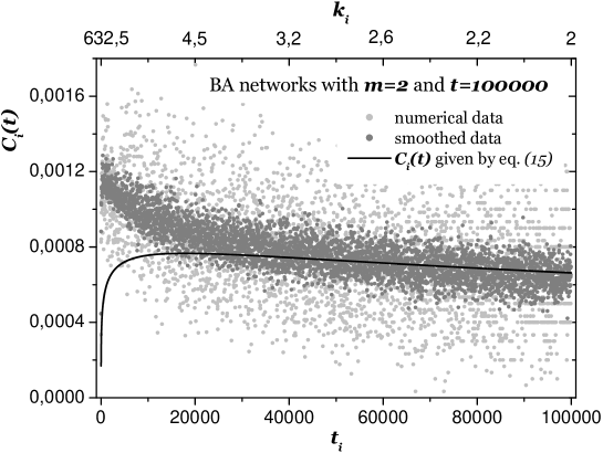
Figure 2: The local clustering coefficient $C_{i}(t)$ as a function $t_{i}$ (averaged over $10^{4}$ networks). Note that the $k_{i}$ axis is nonlinear.

Let us note that if $t_{i}\ll t$ or $m\gg 1$ the local clustering coefficient does not depend on the node under consideration and approaches $C_{i}(t)\simeq(m-1)(\ln t)^{2}/(8t)$ i.e. the formula (6) that gives the the clustering coefficient of a random graph with a power-low degree distribution (4). Since one knows how the node’s degree evolves in time (2) one can also calculate the formula for $C_{i}(k_{i})$. At the Fig.2 we present the formula (15) (solid line) and corresponding numerical data (scatter plots). The two kinds of scatter plots represent respectively: real data (light gray circles) and the same data subjected adjacent averaging smoothing (dark gray circles). As before (see Fig.(1)), we observe a significant disagreement between the numerical data and the theory for small $t_{i}$. We suspect that the effect has the same origin i.e. the relations (2) and (3) that we use in our derivation work well only in the asymptotic region $t_{i}<t\longrightarrow\infty$.

To obtain the clustering coefficient $C$ of the whole network the expression (15) has to be averaged over all nodes within a network $C=\int_{1}^{t}C_{i}(t)dt_{i}/t$. We were not able to find an exact analytic form of this integral but corresponding numerical values (open squares at the Fig.3) fit very well a mean field approximation that we propose below (solid line at the Fig.3)

$$C=\left\langle C_{i}(t)\right\rangle_{i}\simeq\frac{(m-1)}{8}\frac{\left\langle\>(\ln t)^{2}+\frac{4m}{(m-1)^{2}}(\ln t_{i})^{2}\>\right\rangle_{i}}{\left\langle\>(\sqrt{t}+\sqrt{t_{i}}/m)^{2}\>\right\rangle_{i}}.$$ (16)

After performing separate integration of the numerator and the denominator one gets

$$C=\frac{6m^{2}\left((m+1)^{2}(\ln t)^{2}-8m\ln t+8m\right)}{8(m-1)(6m^{2}+8m+3)t}.$$ (17)

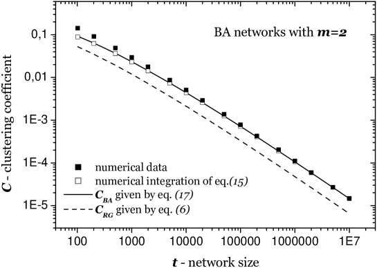
Figure 3: The clustering coefficient $C$ of a whole BA network as a function of the network size $t$ (averaged over $100$ networks).

For large ($t\longrightarrow\infty$) and dense ($m\gg 1$) networks the above formula approaches (6). The effect lets us deduce that the structural correlations dorogov characteristic for growing BA networks become less important in larger and denser networks. The same was suggested in fronczak . Fig.3 shows the average clustering coefficient in BA networks as a function of the network size $t$ compared with the analytical formula (17).

Conclusions. In summary, we applied a mean field approach to study clustering effects in Barabási-Albert networks. We found that the BA networks do not show the homogeneous clustering as suggested in klemm ; ravasz . We derived a general formula for the clustering coefficient $C$ characterizing the whole BA network. We found that in the limit of large ($t\longrightarrow\infty$) and dense ($m\gg 1$) networks both the local ($C_{i}$) and the global ($C$) clustering coefficients approach clustering coefficient derived for a random graph with a power-low degree distribution (4). Our derivations were checked against numerical simulation of BA networks finding a very good agreement.

Acknowledgments. We would like to thank Jarosław Suszek and Daniel Kikoła for their help in computer simulations. AF thanks The State Committee for Scientific Research in Poland for support under grant No. $2P03B01323$. The work of JAH was supported by the special program of the Warsaw University of Technology Dynamics of Complex Systems.

References

- (1) S.Bornholdt and H.G.Schuster, Handbook of Graphs and networks, Wiley-Vch (2002).
- (2) S.N. Dorogovtsev and J.F.F.Mendes, Evolution of Networks, Oxford Univ.Press (2003).
- (3) R.Albert and A.L.Barabási, Rev. Mod. Phys. 74 47 (2002).
- (4) A.L.Barabási and R.Albert, Science 286, 509 (1999).
- (5) A.L.Barabási, R.Albert and H.Jeong, Physica A 272 173 (1999).
- (6) A.Fronczak, P.Fronczak and J.A.Hołyst, cond-mat/0212230.
- (7) R.Cohen and S.Havlin, Phys. Rev. Lett. 90 058701 (2003).
- (8) D.J.Watts and S.H.Strogatz, Nature 393 440 (1998).
- (9) A.Fronczak, J.A. Hołyst, M. Jedynak, J.Sienkiewicz, Physica A 316 688 (2002).
- (10) K.Klemm and V.M.Eguíluz, Phys. Rev. E 65 057102 (2002).
- (11) G.Szabó, M.Alava and J.Kertész, Phys. Rev. E 67 056102 (2003).
- (12) M.E.J.Newman, cond-mat/0202208.
- (13) E.Ravasz and A.L.Barabási, Phys. Rev. E 67 026112 (2003).
- (14) G.Bianconi and A.Capocci, Phys. Rev. Lett. 90 078701 (2003).
- (15) S.N.Dorogovtsev, J.F.F.Mendes and A.N.Samukhin, cond-mat/0206467 (2002).