Vapour-liquid coexistence in many-body dissipative particle dynamics

Abstract

Many-body dissipative particle dynamics is constructed to exhibit vapour-liquid coexistence, with a sharp interface, and a vapour phase of vanishingly small density. In this form, the model is an unusual example of a soft-sphere liquid with a potential energy built out of local-density dependent one-particle self energies. The application to fluid mechanics problems involving free surfaces is illustrated by simulation of a pendant drop.

I Introduction

Dissipative particle dynamics (DPD) is familiar as a method of simulating complex fluids at a coarse grained level Hoogerbrugge and Koelman (1992); Groot and Warren (1997), for example block copolymer polymer melts Groot and Madden (1998); Groot et al. (1999), and surfactant solutions Jury et al. (1999a); Prinsen et al. (2002). DPD has also been used for multiphase fluid problems, such as phase separation kinetics in binary liquid mixtures Coveney and Novik (1996); Jury et al. (1999b); Novik and Coveney (2000), droplet deformation and rupture in shear fields Clark et al. (2000), and droplets on surfaces under the influence of shear fields Jones et al. (1999). The advantage of DPD for these kind of problems lies in the simplicity of the underlying algorithm, and the physical way in which singular events such as droplet rupture are captured. Such considerations also make the method attractive for free-surface fluid dynamics problems. Examples of these include various kinds of wetting, spreading, wicking, and capillary problems. To be used for these kind of problems, DPD needs to be extended to allow for vapour-liquid equilibrium. In this way a free surface will arise naturally as a vapour-liquid interface, and such an interface will possess the same physics as a clean vapour-liquid interface.

To achieve vapour-liquid coexistence in DPD, for a single component system, requires a van der Waals loop in the equation of state (EOS) (pressure-density curve). However this presents a fundamental limitation for standard DPD since the soft interaction forces used in the method invariably lead to a predominantly quadratic EOS Louis et al. (2000). One way around this is the ‘many-body’ DPD method invented by Pagonabarraga and Frenkel Pagonabarraga and Frenkel (2001); RDG , and also investigated by Trofimov et al Trofimov et al. (2002). In many-body DPD, the amplitude of the soft repulsions is made to depend on the local density. In this way one can achieve a much wider range of possibilities for the EOS.

In the present work, many-body DPD is developed to exhibit vapour-liquid coexistence, with a sharp interface, and a vapour phase of vanishingly small density. The approach taken is fundamentally the same approach as used in Refs. Pagonabarraga and Frenkel, 2001 and Trofimov et al., 2002, but with a somewhat different interpretation of the same mathematics. Therefore a general theory for many-body DPD is described first, which I argue involves a fundamental re-interpretation of the DPD interaction potentials. The specific implementation for vapour-liquid equilibrium is described next, and finally the application to free surface problems is illustrated by simulation of a pendant droplet. Another application to vapour-liquid phase separation kinetics was described in an earlier note Warren (2001).

II General theory

Dissipative particle dynamics (DPD) is basically Molecular Dynamics Allen and Tildesley (1987); Frenkel and Smit (1996), with two key innovations. The first, and perhaps the most profound, is the use of soft interactions. This stands in contrast to the common use of interaction potentials corresponding to particles with hard cores, for example Lennard-Jones interactions or modified hard-sphere interactions. The second innovation is the use of a momentum conserving thermostat. This allows one to simulate at a well defined temperature yet preserve hydrodynamics, and this can be important for some problems such as phase separation kinetics. The thermostat described below is the original (Español-Warren) thermostat Español and Warren (1995), although the Lowe-Anderson thermostat is perhaps simpler and more efficient Lowe (1999). In the present paper, the focus is on the equilibrium properties of many-body DPD models, and the nature of the thermostat is unimportant.

The particles in DPD have positions ${\mathbf{r}}_{i}$ and velocities ${\mathbf{v}}_{i}$, where $i=1$ to $N$ runs over the set of particles, moving in a simulation box of volume $V$. They move according to the kinematic condition $d{\mathbf{r}}_{i}/dt={\mathbf{v}}_{i}$, and Newton’s second law $d{\mathbf{v}}_{i}/dt={\mathbf{F}}_{i}/m_{i}$ where $m_{i}$ is the mass of the $i$th particle. Here

$${\mathbf{F}}_{i}={\mathbf{F}}_{i,{\mathrm{ext}}}+{\textstyle\sum_{j\neq i}}\,{\mathbf{F}}_{ij}$$ (1)

is the total force acting on the $i$th particle, comprising a possible external force ${\mathbf{F}}_{i,{\mathrm{ext}}}$ and forces ${\mathbf{F}}_{ij}$ due to the interaction between the $i$th and $j$th particles. The interaction forces are decomposed into conservative, dissipative and random contributions,

$${\mathbf{F}}_{ij}={\mathbf{F}}_{ij}^{\mathrm{C}}+{\mathbf{F}}_{ij}^{\mathrm{D}}+{\mathbf{F}}_{ij}^{\mathrm{R}}.$$ (2)

The individual contributions all vanish for particle separations larger than some cutoff interaction range $r_{{c}}$, and all obey Newton’s third law so that ${\mathbf{F}}_{ij}+{\mathbf{F}}_{ji}=0$.

The conservative force is

$${\mathbf{F}}_{ij}^{\mathrm{C}}=A\,w_{\mathrm{C}}(r_{ij})\,{\mathbf{e}}_{ij}$$ (3)

where ${\mathbf{r}}_{ij}={\mathbf{r}}_{j}-{\mathbf{r}}_{i}$, $r_{ij}=|{\mathbf{r}}_{ij}|$, and ${\mathbf{e}}_{ij}={\mathbf{r}}_{ij}/r_{ij}$. The weight function $w_{\mathrm{C}}(r)$ vanishes for $r>r_{{c}}$, and for simplicity is taken to decreases linearly with particle separation, thus $w_{\mathrm{C}}(r)=(1-r/r_{{c}})$. This force corresponds to a total potential energy which is a sum of pair potentials

$$U(\{{\mathbf{r}}_{i}\})={\textstyle\sum_{j>i}}\,\phi(r_{ij})$$ (4)

where $-\phi\,{}^{\prime}(r)=Aw_{\mathrm{C}}(r)$, and thus $\phi(r)=(A/2)(1-r/r_{{c}})^{2}$ for standard DPD. The dissipative and random forces are ${\mathbf{F}}_{ij}^{\mathrm{D}}=-\gamma w_{\mathrm{D}}(r_{ij})({\mathbf{v}}_{ij}\cdot{\mathbf{e}}_{ij}){\mathbf{e}}_{ij}$ and ${\mathbf{F}}_{ij}^{\mathrm{R}}=\sigma w_{\mathrm{R}}(r_{ij})\xi_{ij}{\mathbf{e}}_{ij}$. In these $\gamma$ and $\sigma$ are amplitudes, $w_{\mathrm{D}}(r)$ and $w_{\mathrm{R}}(r)$ are additional weight functions also vanishing for $r>r_{{c}}$, ${\mathbf{v}}_{ij}={\mathbf{v}}_{j}-{\mathbf{v}}_{i}$, and $\xi_{ij}=\xi_{ji}$ is pairwise continuous white noise with $\langle\xi_{ij}(t)\rangle=0$ and $\langle\xi_{ij}(t)\xi_{kl}(t^{\prime})\rangle=(\delta_{ik}\delta_{jl}+\delta_{il}\delta_{jk})\delta(t-t^{\prime})$. The dissipative and random forces act as the above-mentioned thermostat provided that the weight functions and amplitudes are chosen to obey a fluctuation-dissipation theorem: $\sigma^{2}=2\gamma k_{\mathrm{B}}T$ and $w_{\mathrm{D}}=(w_{\mathrm{R}})^{2}$, where $k_{\mathrm{B}}T$ is the desired temperature in units of Boltzmann’s constant $k_{\mathrm{B}}$ Español and Warren (1995). The same weight function is used as for the conservative forces (basically for historical reasons): $w_{\mathrm{R}}=w_{\mathrm{C}}$ and $w_{\mathrm{D}}=(w_{\mathrm{C}})^{2}$.

Usually all the particles are assumed to have the same mass, and to fix units of mass and length a convenient choice is to set $m_{i}=r_{{c}}=1$. Often the units of energy and hence time are fixed by setting $k_{\mathrm{B}}T=1$, but for equilibrium simulations it can be convenient to keep $k_{\mathrm{B}}T$ as a free parameter.

The integration of the equations of motion is a non-trivial matter since one has to manage the random forces somehow. For an integration algorithm, Groot and Warren investigated a version of the velocity-Verlet scheme used in molecular dynamics simulations Groot and Warren (1997), but it was later shown by den Otter and Clarke that this is not a real improvement over a simple Euler type integration scheme den Otter and Clarke (2001). More extensive studies have been undertaken by Vattulainen et al Vattulainen et al. (2002). But many the problems are obviated if the Lowe-Anderson thermostat is used, which is based on distinctly different physical ideas Lowe (1999). All the simulations described below though were carried out with the simple velocity-Verlet like algorithm described by Groot and Warren.

For a single-component DPD fluid, the equation of state (EOS) gives the pressure $p$ as a function of the density $\rho=N/V$. For the soft potential given above, the EOS is now well established to be Groot and Warren (1997)

$$p=\rho k_{\mathrm{B}}T+\alpha A\rho^{2}$$ (5)

where $\alpha=0.101\pm 0.001$ is very close to the mean field prediction $\alpha_{\mathrm{MF}}=\pi/30=0.1047$ (see also below). The first term in the EOS is an ideal gas term, and the second term is the excess pressure, which is almost perfectly quadratic in the density (there is a very small correction of order $\rho^{3}$). Note though that $\alpha A$ is not the second virial coefficient Louis et al. (2000), so the above EOS breaks down as $\rho\to 0$. It seems that a quadratic EOS like this is unavoidable for soft potentials Louis et al. (2000). This represents the fundamental limitation to basic DPD mentioned in the introduction. Moreover one has to take $A\geq 0$ otherwise the pressure diverges negatively at high densities, so one is are restricted to a strictly positive compressibility $\partial p/\partial\rho>0$. In fact, making $A<0$ throws the DPD pair potential into a formal class of catastrophic potentials for which it can be rigorously proved there is no thermodynamic limit Louis et al. (2000); Ruelle (1999). The situation is not as grim as it might seem though since considerable progress can be made for applications by introducing different species of particles, and allowing them to be differentiated by their repulsion amplitudes thus $A\to A_{ij}$ in Eqs. (3) and (4).

For the one-component fluid, an obvious way to get around the problem of a quadratic EOS is to make the amplitude $A$ in the force law dependent on density somehow. Such a scheme has been examined by several workers Pagonabarraga and Frenkel (2001); Trofimov et al. (2002), and proves to be a simple extension to DPD. This many-body DPD requires only a modest additional computational cost, but throws open the possibility to simulate systems with an arbitrarily complicated EOS. Care must be taken though with density-dependent interactions Louis (2002). The approach described here introduces a local density into the amplitude in the force law. By being explicit about the construction of the local density, this is a ‘safe’ way to introduce a density-dependence into the interations Almarza et al. (2001).

In many-body DPD, I write

$${\mathbf{F}}_{ij}^{\mathrm{C}}=\frac{1}{2}[A(\overline{\rho}_{i})+A(\overline{\rho}_{j})]\,w_{\mathrm{C}}(r_{ij})\,{\mathbf{e}}_{ij},$$ (6)

for a one-component fluid (Trofimov et al describe a multi-component generalisation). A partial amplitude $A(\overline{\rho})$ is introduced, depending on a weighted local density, which I define for the $i$th particle to be

$$\overline{\rho}_{i}={\textstyle\sum_{j\neq i}}\,w_{\rho}(r_{ij}).$$ (7)

The weight function $w_{\rho}(r)$ vanishes for $r>r_{{c}}$ and for convenience is normalised so that $\int d^{3}{\mathbf{r}}\,w_{\rho}(r)=1$, although in principle the normalisation could be absorbed into the definition of $A(\overline{\rho}_{i})$. The discounted self contribution $i=j$ in Eq. (7) would only add a constant $w_{\rho}(0)$ to $\overline{\rho}_{i}$, amounting to a constant shift of the argument in the definition of $A(\overline{\rho}_{i})$ (see Trofimov et al for a more extensive discussion on this point). The weighted local density is readily computed by an additional sweep through the neighbour list, hence there is only a modest additional computational overhead. If $A(\overline{\rho})=A$, the method reduces exactly to the standard DPD model.

In mean field theory, it is easy to show that the modified force law should give an EOS

$$p_{\mathrm{MF}}=\rho k_{\mathrm{B}}T+\alpha_{\mathrm{MF}}A(\rho)\rho^{2}$$ (8)

where

$$\alpha_{\mathrm{MF}}=({2\pi}/{3}){\textstyle\int_{0}^{\infty}}dr\,r^{3}\,w_{\mathrm{C}}(r),$$ (9)

(ie $\alpha_{\mathrm{MF}}=\pi/30$ for the standard choice of $w_{\mathrm{C}}(r)$). Thus, in principle, an arbitrary dependence on density can be recovered.

This is not the end of the story though. The existence of a potential energy $U(\{{\mathbf{r}}_{i}\})$ such that ${\mathbf{F}}_{i}=\partial U/\partial{\mathbf{r}}_{i}$ requires the forces to obey a ‘Maxwell relation’ of the type $\partial{\mathbf{F}}_{i}/\partial{\mathbf{r}}_{j}=\partial{\mathbf{F}}_{j}/\partial{\mathbf{r}}_{i}$. This is a non-trivial requirement since the particle positions appear both directly in Eq. (6) and indirectly through the definition of the local density in Eq. (7). One can show a necessary and sufficient condition for it to be true is that the derivative $w_{\rho}^{\prime}$ is proportional to $w_{\mathrm{C}}$, so the two weight functions $w_{\rho}$ and $w_{\mathrm{C}}$ are not independent. One can then prove from the normalisation condition on $w_{\rho}(r)$ that

$$-w_{\rho}^{\prime}(r)=w_{\mathrm{C}}(r)/2\alpha_{\mathrm{MF}}$$ (10)

where $\alpha_{\mathrm{MF}}$ is defined in Eq. (9).

What, then, is the corresponding potential? I find that

$$U(\{{\mathbf{r}}_{i}\})={\textstyle\sum_{i}}\,u(\overline{\rho}_{i})$$ (11)

where $u(\overline{\rho}_{i})$ is a self energy depending on the local density, such that

$$u^{\prime}(\overline{\rho})=\alpha_{\mathrm{MF}}A(\overline{\rho}).$$ (12)

Comparing Eq. (11) with Eq. (4), it is clear that there has been a profound shift in perspective, from a potential function expressed in terms of soft pair potentials, to one expressed in terms of density-dependent self energies.

There have recently been many discussions on the thermodynamic consistency of density-dependent interactions in the literature Louis (2002); Stillinger et al. (2002); Tejero (2003); Tejero and Baus (2003). However, for the present formulation all thermodynamic relations are valid because the underlying potential $U(\{{\mathbf{r}}_{i}\})$ is a well defined, density-independent function of the particle positions. This is important because it means for instance the virial equation for the pressure or stress tensor, constructed out of the forces, can be used without change.

If $u(\overline{\rho})$ is a polynomial in $\overline{\rho}$ of order $n$, it is easy to show that $\sum_{i}u(\overline{\rho}_{i})$ expands to a sum over $(n+1)$-body density-independent potentials. For $u(\overline{\rho})=\alpha_{\mathrm{MF}}A\overline{\rho}$, standard DPD is recovered.

I wish to emphasise, contrary to some hints in the literature Pagonabarraga and Frenkel (2001); Trofimov et al. (2002), that $\langle U(\{{\mathbf{r}}_{i}\})\rangle$ is the internal energy and not the excess free energy (here $\langle\dots\rangle$ is a thermal average). It follows from Eqs. (8) and (11) that the mean field EOS is $p_{\mathrm{MF}}=\rho k_{\mathrm{B}}T+\rho^{2}u^{\prime}(\rho)$. A standard thermodynamic result for the true pressure is $p=\rho k_{\mathrm{B}}T+\rho^{2}f_{N}^{\mathrm{(ex)}}{}^{\prime}(\rho)$ where $f_{N}^{\mathrm{(ex)}}(\rho)$ is the excess free energy per particle. This shows that the interpretation $u\equiv f_{N}^{\mathrm{(ex)}}$ is a mean field approximation, and as such will be spoilt by correlation effects. Note also that correlations mean, typically, $\langle\overline{\rho}_{i}\rangle\neq\rho$, and $\langle u(\overline{\rho}_{i})\rangle\neq u(\langle\overline{\rho}_{i}\rangle)\neq u(\rho)$. Trofimov et al give results for the mean local density, and suggest ways that one might improve the correspondence between $\langle\overline{\rho}_{i}\rangle$ and $\rho$. Here I take a different approach, and regard $\overline{\rho}_{i}$ as a convenient intermediate quantity which is used to construct the forces; as such it is not important that its average differs from $\rho$. In practice, like Trofimov et al, I find that the mean field EOS for many-body DPD can be considerably less accurate compared to standard DPD. Thus the method always requires calibration to determine the true thermodynamic properties (the approach of Trofimov et al can be used to achieve a specific EOS).

(a)

(b)

Figure 1: Data collapse of pressure against density. (a) standard DPD model, for $\rho=1$–10 and $A=0$–50. Straight line is fit to data given by Eq. (5) in the text. (b) Many-body DPD model, for $\rho=1$–10, $A=0$–50, $Br_{{d}}^{4}=0$–10 and $r_{{d}}=0.5$–1.0. The ordinate is the function $F=(p-\rho-\alpha A\rho^{2}-2\alpha Br_{{d}}^{4}\rho^{3})/Br_{{d}}^{4}$. Plotted this way, the data collapse onto quasi-universal straight lines, where the slope depends primarily on $r_{{d}}$. This can be expressed as a quasi-universal EOS in Eq. (17) in the text.

III A specific model

I now describe in more detail a specific application of these ideas to set up a DPD model which exhibits vapour-liquid coexistence. Before this though, there is one more technical point to discuss.

To stabilise the vapour-liquid interface, it is not sufficient just to have a van der Waals loop in the EOS; one must also give consideration to the ranges of the interactions. Thus simple many-body DPD with a single range may not have a stable interface as discussed by Pagonabarraga and Frenkel Pagonabarraga and Frenkel (2001). The trick employed here is to take the standard DPD model, make the soft pair potential attractive, and add on a repulsive many-body contribution with a different range $r_{{d}}<r_{{c}}$. Furthermore I choose the simplest form of the many-body repulsion, namely a self energy per particle which is quadratic in the local density.

In terms of force laws, I take the standard DPD model as specified in Eq. (3) with $A<0$, and add a many-body force law of the form

$${\mathbf{F}}_{ij}^{\mathrm{C}}=B(\overline{\rho}_{i}+\overline{\rho}_{j})\,w_{\mathrm{C}}(r_{ij})\,{\mathbf{e}}_{ij}$$ (13)

where $B>0$. This is Eq. (6) with $A(\overline{\rho})=2B\overline{\rho}$. The weight function in this is chosen to be $w_{\mathrm{C}}(r)=(1-r/r_{{d}})$ for $r<r_{{d}}$. This means that $w_{\rho}(r)=15/(2\pi r_{{d}}^{3})(1-r/r_{{d}})^{2}$ (normalised for three dimensions) is used to construct the local density, and $\alpha_{\mathrm{MF}}=\pi r_{{d}}^{4}/30$ for this particular interaction.

In terms of potentials, this model can be interpreted as follows. Define a generalised weight function of range $R$ via

$$w_{\rho}(r;R)={15}/{(2\pi R^{3})}(1-{r}/{R})^{2}.$$ (14)

Then define two local densities $\overline{\rho}$ and ${\overline{\overline{\rho}}}$, constructed using this weight function with $R=r_{{c}}$ and $R=r_{{d}}$ respectively. The self energy per particle for this specific model can be written as

$$u=(\pi/30)A\overline{\rho}+(\pi r_{{d}}^{4}/30)B{\overline{\overline{\rho}}}{}^{2}.$$ (15)

This is at most quadratic in the local densities, and thus the model could be written out explicitly in terms of two- and three-body interaction potentials. From this, the mean field EOS is

$$p_{\mathrm{MF}}=\rho k_{\mathrm{B}}T+(\pi/30)(A+2Br_{{d}}^{4}\rho)\rho^{2}.$$ (16)

Thus, with $A<0$ and $B>0$, this EOS has the potential to contain a van der Waals loop. The actual EOS differs from this systematically as I now describe.

$r_{{d}}$	0.50	0.65	0.75	0.85	1.00
$c$	4.0(5)	4.1(1)	3.07(5)	2.08(5)	1.29(5)

Table 1: Density correction ‘constant’ for many-body term in measured EOS, as a function of $r_{{d}}$. There is little significant dependence on other parameters $A$, $B$ and $\rho$ (see eg Fig. 1(b)). Figures in brackets are estimates of the error in the final digit.

(a)

(b)

Figure 2: (a) Data collapse of pressure against density, for $\rho_{\mathrm{L}}<\rho\lesssim 8$, $A<0$ and $|A|=20$–40, $B=25$ or 40, and $r_{{d}}=0.75$. The ordinate is the function $F=(p-\rho-\alpha A\rho^{2}-2\alpha Br_{{d}}^{4}\rho^{3})/Br_{{d}}^{4}$ Straight line is fit to data given by Eq. (18) in the text. (b) Pressure as a function of density for the two selected parameter sets in Table 2. The lines are the predictions of the fitted EOS, Eq. (18) in the text.

IV Simulation results

I now explore by simulation the properties of the above model. First I examine the actual EOS, then vapour-liquid coexistence and the properties of a stable vapour-liquid interface, and finally illustrate the potential application of the method with a simple pendant droplet simulation. Typical simulations presented here are in simulation boxes of size $10^{3}$ (units of $r_{{c}}$).

IV.1 Equation of state

For $B=0$, the standard DPD model, the simulations recover the accepted equation of state Eq. (5) with very small corrections of $\sim\rho^{3}$. Results are shown in Fig. 1(a).

For $A>0$ and $B>0$ a large number of simulations were performed. After some experimentation, the data was found to collapse to the following quasi-universal behaviour,

$$p=\rho+\alpha A\rho^{2}+2\alpha Br_{{d}}^{4}\rho^{2}(\rho-c).$$ (17)

where $\alpha$ takes the same value as for standard DPD (and thus this expression contains the correct $B=0$ limit), and $c$ is an empirical correction to the density that appears in the many-body term. This should be compared to the mean field prediction in Eq. (16). I find that $c$ depends predominantly on $r_{{d}}$ according to Table 1. A representative sample of the data is shown in Fig. 1(b).

For some parameter sets, the temperature was found to show strong deviations from the nominal $k_{\mathrm{B}}T=1$, as a result of instabilities in the integration algorithm. Results were only kept if the measured $k_{\mathrm{B}}T$ lay within 10% of the nominal value. These problems occur if the repulsion amplitudes are too large, or the densities too high, or $r_{{d}}$ too small. The integration algorithm is that described in Groot and Warren Groot and Warren (1997), with a time step $\Delta t=0.05$ and $\lambda=1/2$. The instabilities can be vanquished by making $\Delta t$ smaller.

The measured equation of state is therefore quite close to the predicted mean field equation of state. The main difference is a correction to the density dependence of the many-body term. This is expected since the pair correlation function $g(r)<1$ where the repulsions are strongest, and thus $\langle\overline{\rho}_{i}\rangle<\rho$. This effect has also been checked in simulations by monitoring the mean value of the local density, with results similar to those reported by Trofimov et al Trofimov et al. (2002).

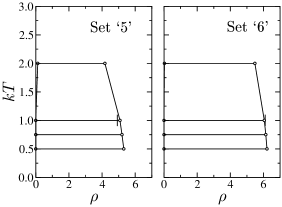
Figure 3: Density-temperature phase diagrams for the two parameter sets in Table 2. Shown horizontal are tielines computed from vapour-liquid interface profiles, at several temperatures (keeping $A$ and $B$ fixed). The short vertical line on the $k_{\mathrm{B}}T=1$ tieline is the point where the pressure vanishes according to the fitted EOS, Eq. (18) in the text.

IV.2 Vapour-liquid coexistence

For vapour-liquid coexistence I set $A<0$ and $B>0$ so that there is a van der Waals loop in the EOS. Phase separation is found in a range of densities $\rho_{\mathrm{V}}<\rho<\rho_{\mathrm{L}}$ where $\rho_{\mathrm{V}}$ and $\rho_{\mathrm{L}}$ are the vapour and liquid coexistence densities.

In principle, integration of the EOS gives the free energy density from which predictions can be made about $\rho_{\mathrm{V}}$ and $\rho_{\mathrm{L}}$. Unfortunately, the EOS must deviate from the above fitted form for $\rho\ll 1$, therefore the vapour phase is inadequately characterised. For applications, one is most interested in $\rho_{\mathrm{L}}\gtrsim 1$ in coexistence with a very dilute vapour. If this is true it is much easier to use the EOS to predict the point where the pressure vanishes as an estimate of the coexisting liquid phase density, thus $p(\rho_{\mathrm{L}})=0$. Using this, one expects liquid densities in the range $\rho_{\mathrm{L}}\sim 5$ for $-A\sim B\sim 30$. From here on I have set the range of the many-body repulsion to $r_{{d}}=0.75$ as a mid-range value determined above.

Since the above EOS was measured for $A>0$, one has to be careful to check that the scaling collapse still holds. One cannot easily measure the EOS within the phase separation region, since it is hard to maintain a stable uniform density. Therefore the EOS has been characterised for $\rho>\rho_{\mathrm{L}}$. A similar data collapse is found to the previous section, as is shown in Fig. 2(a). In this case, the EOS can be fitted by

$$p=\rho+\alpha A\rho^{2}+2\alpha Br_{{d}}^{4}(\rho^{3}-c\rho^{2}+d)$$ (18)

where $\alpha=0.101(1)$ as before, $c=4.16(2)$ and $d=18(1)$. The value of $c$ is similar to the value obtained previously ($c=3.07(5)$, Table 1). There is an additional offset term $d$ which is about 10% of the density correction term $c\rho^{2}$ in the region of interest.

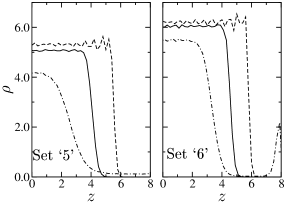
Figure 4: Interfacial density profiles for the two parameter sets in Table 2, for several values of the temperature (keeping $A$ and $B$ fixed): $k_{\mathrm{B}}T=1$ (solid line), $k_{\mathrm{B}}T=2$ (chained line), $k_{\mathrm{B}}T=0.5$ (dashed line).

set	$A$	$B$	$r_{{d}}$	$\rho_{\mathrm{L}}$	$w$	$\sigma$	$\partial p/\partial\rho$
‘5’	$-40$	40	0.75	5.08(1)	0.78(5)	4.95(3)	49(2)
‘6’	$-40$	25	0.75	6.05(1)	0.66(3)	7.45(4)	47(2)

Table 2: The two parameter sets used in subsequent simulations. The sets are distinguished by the different values of the liquid densities $\rho_{\mathrm{L}}$. The coexisting vapour density $\rho_{\mathrm{V}}\ll 1$, so these parameters are suitable for free surface simulations. Also shown are the interface width $w$, surface tension $\sigma$, and compressibility at $\rho=\rho_{\mathrm{L}}$ estimated from the EOS. All results are at $r_{{c}}=k_{\mathrm{B}}T=1$.

Although a wider parameter space was explored, I concentrate here on two parameter sets that were selected for more detailed work. These parameter sets are given in Table 2 (first three columns). Fig. 2(b) shows the prediction of the EOS, Eq. (18), compared directly against the measured pressures, for these two parameter sets.

For these two parameter sets, the coexisting vapour and liquid densities were determined from the vapour-liquid interface profile simulations described in the next section, and are shown as a function of $k_{\mathrm{B}}T$ in Fig. 3. Where $k_{\mathrm{B}}T\neq 1$ in these simulations, the values of $A$ and $B$ are left at the values in Table 2, in other words $A$ and $B$ are regarded as absolute interaction energies. Also shown in Fig. 3 are the appropriate solutions of $p=0$ using the EOS in Eq. (18).

It is clear that the difference $\rho_{\mathrm{L}}-\rho_{\mathrm{V}}$ gets smaller as $T$ increases, as one approaches the expected vapour-liquid critical point. At $k_{\mathrm{B}}T\lesssim 1$, $\rho_{\mathrm{V}}\ll 1$ indicating the vapour phase is virtually devoid of particles. At $k_{\mathrm{B}}T=1$ the solution to $p=0$ for the EOS gives a good estimate of the density of the fluid phase.

I have also used the EOS to estimate the compressibility $\partial p/\partial\rho$ at $\rho=\rho_{\mathrm{L}}$, and the values are shown in Table 2. Although the precise value is not important, the fact that $\partial p/\partial\rho\gg 1$ at the coexisting fluid density (where $p\approx 0$) shows that the fluid phase is relatively incompressible, similar to a real liquid.

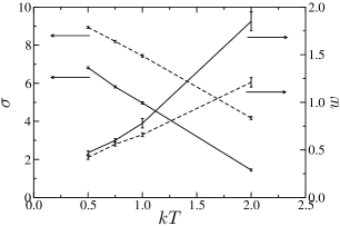
Figure 5: Interfacial tension $\sigma$ (left hand axis) and interface width $w$ (right hand axis), as a function of temperature $k_{\mathrm{B}}T$, for the two parameter sets in Table 2 (keeping $A$ and $B$ fixed): set ‘5’ (solid lines) and set ‘6’ (dashed lines).

IV.3 Vapour-liquid interface

Simulations of the vapour-liquid interface were undertaken, by taking an equilibrated volume of fluid in a periodic box, at a density close to the $p=0$ limit, and removing the particles in one half of the box. The system was allowed to evolve until an equilibrium density profile was obtained. Interface profiles and surface tension values were measured as described for fluid-fluid interfaces Clark et al. (2000). For measurement of density profiles, it was necessary to stop the interface drifting over time. This was achieved by inserting a thin slab of ‘frozen’ particles at one end of the box.

Fig. 4 shows the interface profiles obtained this way for the two selected parameter sets in Table 2. These are shown at several different values of $k_{\mathrm{B}}T$ keeping $A$ and $B$ fixed. The limiting densities on either side of the interface were used to construct the tielines discussed in the previous section (Fig. 3). As the temperature is increased, the interfacial width $w$ gets broader, and the surface tension $\sigma$ drops. Results for $\sigma$ and $w$ are shown in Fig. 5. The width $w$ was quantified by calculating the maximum slope, and normalising to the coexistence densities, thus

$$w=\frac{\rho_{\mathrm{L}}-\rho_{\mathrm{V}}}{\mathrm{max}\,|d\rho/dz|}.$$ (19)

The surface tension is determined from the standard mechanical definition of the pressure tensor Allen and Tildesley (1987). Note again that there is no problem with the many-body origin of the force laws. The actual forces enter the calculation in exactly the same way as standard DPD.

Low temperature favours a sharp interface, but if the temperature is too low, oscillations develop in the profile on the liquid side of the interface. This can be seen most clearly in Fig. 4 for $k_{\mathrm{B}}T=0.5$. The system has crossed a Fisher-Widom line in the phase diagram, and a freezing transition is almost certainly nearby. The relative amplitude of the oscillations can be measured, and they are typically 10% of the bulk density at $k_{\mathrm{B}}T=0.5$, but $<2$% for $k_{\mathrm{B}}T\geq 0.75$, at least for the two sets of parameters studied here.

Thus I conclude that the two parameter sets given in Table 2 provide for a sharp vapour-liquid interface, at $k_{\mathrm{B}}T=1$, with virtually no particles in the vapour phase. They are thus well suited to model free surfaces. Table 2 also contains the measured interfacial properties.

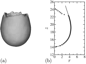
Figure 6: Pendant droplet problem: (a) isosurface cut through $3d$ density field at $\rho=\rho_{\mathrm{L}}/2$, showing the drop profile, and (b) drop radius $r$ as a function of height $z$, computed by the method described in the text. The solid line is the Young-Laplace equation prediction, the circles are the measured profile. The ‘frozen’ support particles at the top of the drop give a ragged edge to the top of the isosurface in (a), and distort the measured profile for $z\gtrsim 23$ in (b). Parameters correspond to set ‘6h’ in Table 3.

set	$g$	$\rho_{\mathrm{L}}$	$\Delta E$	$\beta$	$1/H(\beta)$	$\sigma_{\mathrm{shape}}$	$\sigma_{\mathrm{exact}}$
‘5a’	0.022	5.08	8.80(5)	0.378	0.57(3)	4.9(3)	4.95(3)
‘6f’	0.025	6.05	9.00(5)	0.378	0.57(3)	7.0(5)	7.45(4)
‘6h’	0.033	6.05	8.75(5)	0.404	0.52(2)	7.9(4)	7.45(4)
‘6g’	0.030	6.05	8.70(5)	0.431	0.48(4)	6.6(5)	7.45(4)

Table 3: Pendant drop profile data. Interaction parameters are taken from Table 2, according to the first digit of ‘set’. The penultimate column is the surface tension computed from the drop shape, and the final column is the ‘exact’ surface tension from Table 2, computed by integration of the pressure tensor through a planar interface.

IV.4 Pendant droplet simulation

As an example application, I look at the classic pendant drop problem. The procedure is very similar to the one adopted for the DPD multiphase fluid model Clark et al. (2000).

To set up the pendant droplet, a volume of fluid at a density close to the equilibrium liquid density was equilibrated, then replicated to construct a cylindrical column with the axis parallel to the $z$-direction. A ‘support’ was constructed by ‘freezing’ particles in a thin slice at the top of the column. A gravitational body force $g$ was included by adding a constant force per particle directed along the $z$-direction away from the support. When the system reaches equilibrium, the liquid forms a pendant droplet suspended from the support particles. In equilibrium, the drop profile (radius as a function of height) was obtained as described below. The whole simulation takes a couple of minutes on a modern workstation. The droplet contains typically $\sim 3000$ particles.

The profile was determined as follows. A $3d$ mesh was introduced with a resolution typically $\leq 0.5r_{{c}}$ (higher resolution was employed in the $z$-direction). The local particle density in each mesh volume element was computed by averaging over a period of time. This gives a $3d$ density field. The droplet can then be imaged as an isosurface or level cut through this density field, and a typical result is shown in Fig. 6(a).

To determine the drop radius as a function of height, the density field was divided (or ‘segmented’) into occupied and unoccupied cells according to whether $\rho({\mathbf{r}})>\rho_{\mathrm{L}}/2$ or not. The number of occupied cells at each height $z$ was used to compute the cross-sectional area of the droplet at that height, and therefore the drop radius as a function of $z$. A typical drop profile is shown in Fig. 6(b).

This indirect procedure to determine the droplet radius eliminates two possible artefacts. Firstly it removes the blurring of the base of the drop by the interface profile, which would otherwise be $\sim 0.7$–$0.8r_{{c}}$. Secondly it eliminates effects due to the variation of fluid density with height which might otherwise introduce a systematic error, if the mean particle number density as a function of height was computed directly. Such a variation of density with height is to be expected, since the fluid responds to the varying pressure field through the EOS (ie it is still a compressible fluid, even if only weakly so).

The drop profile was analysed by normalising with respect to the maximum diameter $\Delta E$, and comparing with a set of precalculated profiles as the Bond number $\beta=\rho_{\mathrm{L}}gb^{2}/\sigma$ varies (where $b$ is the radius of curvature of the base of the droplet). The profiles are calculated from the Young-Laplace equation as described in earlier work Clark et al. (2000). From the best-fit $\beta$ value, the surface tension can be computed from $\sigma=\rho_{\mathrm{L}}g\Delta E^{2}/H$ where $H(\beta)$ is a dimensionless function computed numerically.

Table 3 shows the quantities computed for several drops, for both parameter sets, and for several values of $g$. Although the surface tensions determined this way are not very precise, they are all consistent with the accurate values calculated directly from the interfacial profiles. The drop profiles all match the measured profiles quite accurately, see for example Fig. 6(b).

V Discussion

The model developed here can be discussed in several contexts. Firstly, it is a new simulation method for fluid mechanics problems involving liquids with free surfaces. For example, the above pendant droplet problem is a test of the static force balance and the results show that the DPD fluid obeys the Young-Laplace equation in a non-trivial geometry. One can conclude that this particular version of many-body DPD offers a viable route for solving capillary problems such as the distribution of liquids in porous materials. It is clearly possible to address dynamic force balance situations too, but these will require further testing and parametrisation, particularly for the notorious problem of contact line dynamics.

Secondly, now that vapour-liquid equilibrium is achieved for a basic soft sphere model, one can ‘dress’ the liquid up in various ways such as making the liquid particles into polymers or model amphiphiles. In this way, new methods can be constructed to simulate complex fluids with an implicit solvent. These developments are the subject of ongoing investigations and will be reported separately.

In a third context though, the re-interpretation of many-body DPD as a fluid whose potential energy is built out of local-density dependent one-particle self energies is quite novel from the point of view of liquid state theory. Most previous work has concentrated on fixed pair potentials with hard cores, and only minor attention has been paid to soft potentials or density-dependent pair potentials. The present work though goes some way beyond these existing ideas.

It has long been recognised that an arbitrary $U(\{{\mathbf{r}}_{i}\})$ can be expanded as a sum over density-independent one-body, two-body (pair potential), etc, terms. Normally the one-body terms, or self energies, are harmless constants which can be discarded, and most of the phenomena observed for liquids can be captured by truncating the expansion at the pair potential level. If one allows the pieces in such an expansion to acquire a density dependence though, then the one-body self energy is no longer necessarily a constant, and it is no longer necessary to go to the pair potential level to see interesting physics. Many-body DPD as described here is an example of precisely this.

The phase behaviour of the present model is also potentially very interesting. By analogy with related soft-core systems such as the Gaussian core model Stillinger (1976); Louis et al. (2000), and models for polymers of various architectures Watzlawek et al. (1999); Likos et al. (2002), the particles in the original DPD model are expected to freeze into a variety of ordered phases at low temperatures and intermediate densities, with a re-entrant fluid phase at high densities. The version of many-body DPD presented in this paper is constructed to have a significant vapour-liquid coexistence region, as shown in Fig. 3, but the low temperature ordered phases are presumably still present, as indicated by the presence of oscillations in the liquid side of the vapour-liquid interface in Fig. 4. In such a case, the collision between the vapour-liquid transition and these ordered phases could prove to generate rather unusual phase behaviour, and the low temperature properties of many-body DPD models may well be worth further examination.

I thank R. D. Groot for many discussions in the early stages of development of the many-body DPD model.

References

- Hoogerbrugge and Koelman (1992) P. J. Hoogerbrugge and J. M. V. A. Koelman, Europhys. Lett. 19, 155 (1992).
- Groot and Warren (1997) R. D. Groot and P. B. Warren, J. Chem. Phys. 107, 4423 (1997).
- Groot and Madden (1998) R. D. Groot and T. J. Madden, J. Chem. Phys. 108, 8713 (1998).
- Groot et al. (1999) R. D. Groot, T. J. Madden, and D. J. Tildesley, J. Chem. Phys. 110, 9739 (1999).
- Jury et al. (1999a) S. Jury, P. Bladon, M. Cates, S. Krishna, M. Hagen, J. N. Ruddock, and P. B. Warren, Phys. Chem. Chem. Phys. 1, 2051 (1999a).
- Prinsen et al. (2002) P. Prinsen, P. B. Warren, and M. A. J. Michels, Phys. Rev. Lett. 89, 148302 (2002).
- Coveney and Novik (1996) P. V. Coveney and K. E. Novik, Phys. Rev. E 54, 5134 (1996).
- Jury et al. (1999b) S. I. Jury, P. Bladon, S. Krishna, and M. E. Cates, Phys. Rev. E 59, R2535 (1999b).
- Novik and Coveney (2000) K. E. Novik and P. V. Coveney, Phys. Rev. E 61, 435 (2000).
- Clark et al. (2000) A. T. Clark, M. Lal, J. N. Ruddock, and P. B. Warren, Langmuir 16, 6342 (2000).
- Jones et al. (1999) J. L. Jones, M. Lal, J. N. Ruddock, and N. Spenley, Faraday Discuss. 112, 129 (1999).
- Louis et al. (2000) A. A. Louis, P. G. Bolhuis, and J.-P. Hansen, Phys. Rev. E 62, 7961 (2000).
- Pagonabarraga and Frenkel (2001) I. Pagonabarraga and D. Frenkel, J. Chem. Phys. 115, 5015 (2001).
- (14) The method was also invented independently by R. D. Groot.
- Trofimov et al. (2002) S. Y. Trofimov, E. L. F. Nies, and M. A. J. Michels, J. Chem. Phys. 117, 9383 (2002).
- Warren (2001) P. B. Warren, Phys. Rev. Lett. 87, 225702 (2001).
- Allen and Tildesley (1987) M. P. Allen and D. J. Tildesley, Computer Simulation of Liquids (Clarendon Press, Oxford, 1987).
- Frenkel and Smit (1996) D. Frenkel and B. Smit, Understanding Molecular Simulation (Academic Press, San Diego, 1996).
- Español and Warren (1995) P. Español and P. B. Warren, Europhys. Lett. 30, 191 (1995).
- Lowe (1999) C. P. Lowe, Europhys. Lett. 47, 145 (1999).
- den Otter and Clarke (2001) W. K. den Otter and J. H. R. Clarke, Europhys. Lett. 53, 426 (2001).
- Vattulainen et al. (2002) I. Vattulainen, M. Karttunen, G. Besold, and J. M. Polson, J. Chem. Phys. 116, 3967 (2002).
- Ruelle (1999) D. Ruelle, Statistical mechanics: rigorous results (World Scientific, Singapore, 1999).
- Louis (2002) A. A. Louis, J. Phys. Cond. Mat. 14, 9187 (2002).
- Almarza et al. (2001) N. G. Almarza, E. Lomba, G. Ruiz, and C. F. Tejero, Phys. Rev. Lett. 86, 2038 (2001).
- Stillinger et al. (2002) F. H. Stillinger, H. Sakai, and S. Torquato, J. Chem. Phys. 117, 288 (2002).
- Tejero (2003) C. F. Tejero, J. Phys. Cond. Mat. 15, S395 (2003).
- Tejero and Baus (2003) C. F. Tejero and M. Baus, J. Chem. Phys. 118, 892 (2003).
- Stillinger (1976) F. H. Stillinger, J. Chem. Phys. 65, 3968 (1976).
- Watzlawek et al. (1999) M. Watzlawek, C. N. Likos, and H. Löwen, Phys. Rev. Lett. 82, 5290 (1999).
- Likos et al. (2002) C. N. Likos, N. Hoffmann, H. Löwen, and A. A. Louis, J. Phys. Cond. Matt. 14, 7681 (2002).