Equilibration of Long Chain Polymer Melts in Computer Simulations

Abstract

Several methods for preparing well equilibrated melts of long chains polymers are studied. We show that the standard method in which one starts with an ensemble of chains with the correct end-to-end distance arranged randomly in the simulation cell and introduces the excluded volume rapidly, leads to deformation on short length scales. This deformation is strongest for long chains and relaxes only after the chains have moved their own size. Two methods are shown to overcome this local deformation of the chains. One method is to first pre-pack the Gaussian chains, which reduces the density fluctuations in the system, followed by a gradual introduction of the excluded volume. The second method is a double-pivot algorithm in which new bonds are formed across a pair of chains, creating two new chains each substantially different from the original. We demonstrate the effectiveness of these methods for a linear bead spring polymer model with both zero and nonzero bending stiffness, however the methods are applicable to more complex architectures such as branched and star polymer.

I Introduction

A systematic investigation of the structure-property relations for polymeric systems by computer simulations requires the preparation of equilibrated melts of long, entangled chains. For temperatures well above the glass transition, this can, in principle, be achieved using sufficiently long molecular dynamics (MD) or Monte Carlo (MC) simulations. However since the longest relaxation of an entangled polymer melt of length $N$ scales at least as $N^{3}$, giving at least $N^{4}$ in cpu time, this method is only feasible for relatively short chain lengths. Depending on the detail of the model the longest chains which can presently be equilibrated by brute-force MD or MC simulations are on the order of 2-7 entanglements lengths $N_{e}$. Using united atom potentials for polyethylene in which one treats the carbon and its bonded hydrogen as a single united atom, it is possible to equilibrate high temperature $(T\gtrsim 450K)$ melts for chains of the order of approximately $2N_{e}$ or about 200 monomers.[1, 2] For coarse-grained bead-spring models like the one employed here it is possible to study longer chain lengths, on the order of up to 500 monomers or approximately $7N_{e}$.[3] However this reaches the very limits of present day fastest computers. An increase of cpu speed by an order of magnitude does even not allow for a doubling of the chain length. While the present chain lengths are sufficient to follow the dynamics well into the reptation regime, they are not long enough to study structure-property relations, such as the plateau modulus $G_{N}^{o}$. This would require chains of order $10-20N_{e}$. The situation is even worse for branched polymer melts or polymers at interfaces, where equilibration times even for relatively short chains are prohibitively large to use brute force simulations to produce equilibrated melts.

Fortunately to produce equilibrated samples, there is no need to follow the slow physical dynamics of entangled polymer melts. One possibility is to temporarily turn off the excluded volume interactions and to allow the chains to pass through each other. In order to obtain a well-defined Monte Carlo algorithm, it is useful to combine this idea with parallel tempering. While it has been demonstrated that this is feasible in principle,[4] the method has so far not proven particularly efficient, the main reason being the large amount of computer time spent on unphysical Hamiltonians. More conventional MC algorithms which can be used to equilibrate polymer melts include reptation moves (generalized slithering snake algorithms),[5] configuration bias algorithms,[6, 7, 8] and concerted rotation algorithms.[8, 9, 10] Being relatively local, these methods work best for moderate chain lengths and densities. The complete equilibration of very long chain melts still requires long runs. The fastest method, the generalized slithering snake algorithm, theoretically scales as $N^{2}$. An alternative are algorithms, which are able to move large sections of a chain at once. The prototype for such methods is the pivot algorithm[11, 12, 13, 14, 15] in which a monomer is chosen at random and one of the two segments formed by that partitioning is pivoted rigidly in a random direction about the unit. A Boltzmann weight is used to determine if the move is accepted or not. This method is highly efficient for single chains in a continuum, implicit solvent. Unfortunately, a direct application to dense melts is not feasible since any large scale conformational change is bound to violate the packing constraints imposed by the chain excluded volume. However it is possible to introduce a double bond crossing algorithm in a way that two new bonds or bridges are formed across a pair of chains, creating two new chains each substantially different from the original.[2, 10, 16, 17, 18] For the bead spring model concerned here this can simply be done by cutting two bonds and introducing two new bonds as discussed in more detail in Sec. VII. For atomistic models, the bond length is much shorter then the diameter of a monomer, and it is necessary to construct new bridges between the chain segments. Karayiannis et al.[17, 18] have shown that by constructing two trimer bridges between the two properly chosen dimers along the backbone one can quickly equilibrate long chain polyethylene melts. For the two chains involved this is essentially a double-pivot move, where each chain experiences such a pivot rotation.

In addition to improved equilibration algorithms there is an obvious interest in methods for generating initial melt configurations which are as close to equilibrium as possible.[19, 20, 21, 22, 23, 24] In our previous work on polymer melts,[3, 19, 25, 26] we prepared most melts by first generating an ensemble of chains with the correct end-to-end distance and randomly placing them in the simulation cell. We then introduced a weak, non-diverging excluded volume potential in the form of e.g. a cosine potential, $A(1+\cos(\pi r/2^{1/6}\sigma))$, between non-bonded monomers, where $r$ is the distance between two monomers and $\sigma$ is the bead diameter. The amplitude $A$ was then increased over a short time interval until the minimum distance between monomers was sufficient to switch on the Lennard-Jones potential without creating numerical instabilities. In the first part of this paper we confirm observations by Brown et al.[21] that this method deforms the (longer) chains. As a consequence, long chain melts are not as well equilibrated as originally believed. The deformation turns out to be strongest at short length scales and completely relaxes away only after a time $\tau_{max}(N)$, which is the time for a chain to move its own size.[21] This long time is needed because the local chain-chain topology can only relax by the slow physical dynamics. For linear chains, $\tau_{max}(N)\approx\tau_{e}(N/N_{e})^{3}$, where the entanglement time $\tau_{e}=\tau_{\rm Rouse}(N_{e})$ is the Rouse time of a chain of length $N_{e}$ (experimentally the measured exponent is closer to 3.4 than 3 except for extremely long chains). This however was exactly what we tried to avoid by that approach. Not surprisingly, the longer the chain length $N$, the more severe the effect is. For relatively short chains, such as those investigated in our previous studies of the crossover from Rouse to reptation dynamics $(N\leq 350)$, the simulations were run long enough that the results are independent of the starting state.[3, 19, 25] However for longer chains, which cannot be run long enough compared to the longest relaxation time, this simple procedure for generating starting states is inadequate.

In the present paper we report results from an extensive effort to prepare well-equilibrated melts of bead-spring polymers with chain lengths ranging from $N=350$ to $N=7000$. For this purpose we use both approaches outlined above. First we show how to avoid the local stretching with only minimal computational effort by a suitable modification of our standard method. Then we demonstrate the capacity of the double-pivot algorithm to dynamically equilibrate melts of medium sized chains of length up to $N=700$. The paper is organized as follows: In Sec. II we define the model. In Sec. III, we present some simple theoretical estimates of the structure of bead-spring chains with different intrinsic bending stiffness in dense melts. In Sec. IV, we discuss ways to characterize the single chain structure and extract suitable target functions for long chain melts from long simulations of short chain melts. In Sec. V we examine carefully the standard procedure used in the past to prepare melt configurations. We show that for long chains this method deforms the chains at short length scales and that these deformations relax completely only after the chains have moved their own size. In Sec. VI, we present the new pre-packing procedure, which significantly reduces the density fluctuations particularly for long chains. This combined with a gradual introduction of the excluded volume, results in well equilibrated long chain melts in a reasonable amount of cpu time. In Sec. VI we describe the double-pivot algorithm and compare results for the internal dimensions of the chain with those produced from pre-packing and a gradual introduction of the excluded volume. In Sec. VIII we test the two methods for chains with local bending rigidity. A brief summary of our main conclusions are given in Sec. IX.

II Model

We use a coarse grained model in which the polymer is treated as a string of beads of mass $m$ connected by a spring. The beads interact with a purely repulsive Lennard-Jones excluded volume interaction,

$${\rm U_{LJ}}(r)=\left\{\begin{array}[]{lcl}4\epsilon\left\{(\sigma/r)^{12}-(\sigma/r)^{6}+\frac{1}{4}\right\}&&r\leq r_{c}\\ 0&&r\geq r_{c}\end{array}\right.$$ (1)

cutoff at $r_{c}=2^{1/6}\sigma$. The beads are connected by a finite extensible non-linear elastic potential (FENE),

$$\rm{U_{FENE}}(r)=\left\{\begin{array}[]{lcl}-0.5kR_{o}^{2}\ln\left(1-(r/R_{o})^{2}\right)&\ r\leq R_{o}\\ \infty&\ r>R_{o}&\end{array}\right.$$

in addition to the Lennard-Jones interaction. The model parameters are the same as in ref. [19], namely $k=30\epsilon/\sigma^{2}$ and $R_{o}=1.5\sigma$ unless otherwise noted. The temperature $T=\epsilon/k_{B}$. The basic unit of time is $\tau=\sigma(m/\epsilon)^{1/2}$. We performed constant volume simulations of monodisperse melts at a segment density $\rho=0.85\sigma^{-3}$. The temperature was kept constant by coupling the motion of each bead weakly to a heat bath with a local friction $\Gamma$. Unless otherwise specified $\Gamma=0.5m/\tau$. The equations of motion were integrated using a velocity Verlet algorithm with a time step $\Delta t=0.012\tau$. The average bond length is $<b^{2}>^{1/2}=0.97\sigma$. The polymer melts studied consisted of $M$ chains of length $N$ beads. The chain lengths studied varied from $N=25$ to $7000$. The number of chains are each system is specified in Table I.

Equilibration algorithms for polymer melts which follow the physical dynamics encounter a strong growth of the necessary equilibration times with chain length. Per unit of time $\tau$, the simulation of a melt of $M$ chains of length $N$ requires a computational effort of $10^{2}M\times N$ particle updates. Since the longest relaxation time is of the order $\tau_{max}\approx\tau_{e}(N/N_{e})^{3}$, equilibration of our largest system with $M=80$ and $N=7000$ would require $10^{2}M\times N(\tau_{e}/\tau)(N/N_{e})^{3}\approx 8\times 10^{17}$ particle updates. Assuming a typical performance of $2.5\times 10^{5}$ particle updates per second, which is typical for this model on a single processor, the required cpu time for the equilibration is about $10^{5}$ years. On a modern parallel cluster such as the DEC alpha CPlant cluster at Sandia, the times are somewhat less. On 64 processors, we get about 20 steps per second for our largest system, which means that the total time for the chains to move on average their own size is approximately 1600 years. Increasing the numbers of processors helps somewhat but since the efficiency of the computation decreases as the number of processors is increased for fixed system size, this type of brute force approach for long chain melts is clearly not feasible.

In our previous studies, we considered only fully flexible chains. However to demonstrate the effectiveness of the methodology, we also include a nonzero bending stiffness, which is modelled by

$$U_{bend}(\theta)=k_{\theta}\left(1-\cos\theta\right)$$ (2)

where $\cos\theta_{i}=(\hat{\bf r}_{i}-\hat{\bf r}_{i-1})\cdot(\hat{\bf r}_{i+1}-\hat{\bf r}_{i})$, where $(\hat{\bf r}_{i}-\hat{\bf r}_{i-1})$ is the unit vector in the bond direction.

III Chain characteristic in the melt

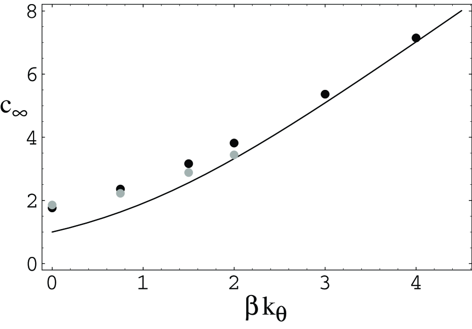
FIG. 1.: Estimates of the effective stiffness $c_{\infty}$ of our chains as a function of the strength $k_{\theta}$ of the bending potential Eq. (2). Eq. (5) (solid line) only accounts for the bending energy, while Eq. (7) ($\bullet$) also considers excluded volume interactions between next-nearest neighbor monomers along the chain. The gray dots indicate estimates based on the analysis of simulation data for equilibrated melts of chain length $N=200-350$ for $k_{\theta}=0$ and $50-100$ for $k_{\theta}>0$.

In dense polymer melts excluded volume interactions between different parts of a given polymer chain are screened. Since in our model there are no explicit intrachain interactions beyond those between neighboring bonds, the single chain structure should be well characterized by the expectation value $\langle\cos\theta\rangle$ of the bond angle $\theta$. For example, the knowledge of $\langle\cos\theta\rangle$ is sufficient to calculate an estimate for the mean-square end-to-end extension $\langle R^{2}\rangle$ of chain segments of length $N$ monomers and $n=N-1$ bonds,

$$\langle R^{2}\rangle(n)=nb^{2}\left(\frac{1+\langle\cos\theta\rangle}{1-\langle\cos\theta\rangle}-\frac{1}{n}\frac{2\langle\cos\theta\rangle\left(1-\langle\cos\theta\rangle^{n}\right)}{\left(1-\langle\cos\theta\rangle\right)^{2}}\right)$$ (3)

where the asymptotic prefactor is referred to as

$$c_{\infty}=\frac{1+\langle\cos\theta\rangle}{1-\langle\cos\theta\rangle}.$$ (4)

The simplest estimate of $\langle\cos(\theta)\rangle$ only takes the bare bending energy Eq. (2) into account. Neglecting small variations in the bond length around the mean value $b=0.97\sigma$, one finds:

$$\langle\cos\theta\rangle = \frac{\int_{0}^{\pi}\sin\theta\cos\theta\exp\left(-\beta U_{bend}(\theta)\right)d\theta}{\int_{0}^{\pi}\sin\theta\exp\left(-\beta U_{bend}(\theta)\right)d\theta}$$ (5)

$$= \frac{1+e^{2\beta k_{\theta}}\left(\beta k_{\theta}-1\right)+\beta k_{\theta}}{\left(e^{2\beta k_{\theta}}-1\right)\beta k_{\theta}},$$ (6)

where $\beta=1/k_{B}T$. Eq. (5) is represented as a solid line in Fig. 1. However this result underestimates the effective chain stiffness, since the chain cannot fold back. This effect can be accounted for approximately by modelling the chains as non-reversal-random-walks (NRRWs) with excluded volume interactions between next-nearest neighbors along the backbone. As a function of the bond angle $\theta$ their distance is given by $l_{\theta}=|\vec{r}_{i+1}-\vec{r}_{i-1}|=b[2(1+\cos\theta_{i})]^{1/2}$ so that

$$\langle\cos\theta\rangle = \frac{\int_{0}^{\pi}\sin\theta\cos\theta\exp\left(-\beta(U_{bend}(\theta)+U_{LJ}(l_{\theta}))\right)d\theta}{\int_{0}^{\pi}\sin\theta\exp\left(-\beta(U_{bend}(\theta)+U_{LJ}(l_{\theta}))\right)d\theta}$$ (7)

which has to be evaluated numerically (see the black dots in Fig. 1). For $k_{\theta}=0$ this gives $c_{\infty}=1.76$ compared to $c_{\infty}=1$ obtained from Eq.( 3) and in good agreement with simulation results for chains of length $20\leq N\leq 350$. This value is slightly smaller than the value $c_{\infty}=2.06$ obtained at the $\Theta$-point for the same Lennard-Jones interaction truncated at $2.5\sigma$ in an implicit, continuum solvent.[15]

Ensembles of single chains which obey Eq. (3) can be generated by simple sampling. This is particularly simple, if the allowed bond vectors are distributed evenly over a solid angle with $\theta\leq\theta_{max}$. In this case

$$\frac{c_{\infty}-1}{c_{\infty}+1}=\langle\cos\theta\rangle_{\theta_{max}}=\left(\cos\theta_{max}/2\right)^{2}$$ (8)

so that the appropriate value for $\theta_{max}$ can be easily determined for any desired effective stiffness.

IV Target functions and suitable ways of characterizing single chain structure

The estimates of the chain structure presented in the previous section were obtained within an effective single chain picture. In reality, the formal characterization of a polymer melt is a complicated many-body problem. For example, we have completely ignored the influence of packing effects on the chain conformations. As was recently shown[27] the local melt structure very sensitively depends on the ratio of bond length to effective excluded volume of the beads. This effect is not well represented by the value of the overall chain extension. Here we use our standard bond length/diameter ratio and focus on the single chain properties, however the methods discussed below apply to systems with different parameters as well. In the present case, sufficiently long MD or MC simulations represent the only “ab initio” method which allows to take into account all interactions.

In order to characterize the chain conformations in the melt we mainly rely on mean-square internal distances $\left<R^{2}\right>(|i-j|,N)$ averaged over all segments of size $n=|i-j|$ along the chains, where $i<j\in[1,N]$ are monomer indices. In addition we characterize deviations from Gaussian statistics on short length scales using the ratio $\left<R^{4}\right>/\left<R^{2}\right>^{2}$. Figures 1 and 2 show a comparison of simulation results for equilibrated melts and our naive estimates. The results from the melts have been run sufficiently long that the chains have moved several times their own size. For $N=350$, $k_{\theta}=0$, the run time $T_{t}=2.6\times 10^{6}\tau$.[3] Clearly, the description of chains in a melt as simple freely jointed chains is too naive. Nevertheless, the deviations are not large and the measured and estimated values for $c_{\infty}$ agree quite well. In particular, the simulation data show neither unexpected features nor significant finite chain length effects.

FIG. 2.: Mean square internal distances from long MD runs for chain length $N=100$ and $350$ respectively for four values of the intrinsic bending stiffness: $k_{\theta}=0$ ($\square$), $k_{\theta}=0.75$ ($\times$), $k_{\theta}=1.5$ ($\ast$), and $k_{\theta}=2.0$ ($+$). We refer to these data sets as “target functions”. For comparison, they are included as thick black lines in subsequent, corresponding plots. The dashed lines show to a fit of Eq. (3) to the asymptotic behavior. The corresponding values for $c_{\infty}$ are included in Fig. 1.

The rest of the present paper deals with algorithms which try to circumvent the slow physical equilibration path. These algorithms will be judged according to two criteria: their capacity to reproduce the target functions and their performance. We mostly concentrate on the fully flexible case. In the end, we come back to the stiffer systems as a kind of “blind test”.

V Standard procedure for Preparing Polymer Melts

Our standard method for preparing melt conformations is as follows:

FIG. 3.: Mean square internal distances after a fast push-off for randomly packed phantom chains of length $N=25\ (+)$, $50\ (\times)$, $350\ (*)$ and $7000(\square)$. The thick line is our target function from Fig. 2.

FIG. 4.: Mean square internal distances for the systems shown in Fig. 3 after an additional MD relation of $10^{4}\tau$ which corresponds to $\tau_{\rm Rouse}(N=90)$. Symbols as in Fig.  3. The thick line is our target function from Fig. 2.

1. Start from an ensemble of chains with the correct end-to-end distance $R^{2}(N)=b^{2}c_{\infty}(N-1)$ on large length scales. For a known $c_{\infty}$ this step is trivial.

2. Arrange the chains randomly in the simulation box.

3. Introduce a weak, non-diverging excluded volume potential. A convenient form for the soft potential is a cosine potential,

   $${\rm U_{soft}}(r)=\left\{\begin{array}[]{ll}A(1+\cos(\pi r/r_{c}))&r\leq r_{c}\\ 0&r\geq r_{c}\end{array}\right.$$

   between non-connected monomers with $r_{c}=2^{1/6}\sigma$. The initial amplitude of $A=4\epsilon$ was linearly increased to a final values of $A\geq 100\epsilon$ (“push-off”) over a short time interval of 10-20 $\tau$. In the final state the inter monomer distances are large enough to allow one to switch to the LJ potential without creating numerical instabilities. During this phase, we often use a stronger coupling to the thermostat by increasing the friction constant to $\Gamma=2.0m/\tau$. In addition, the velocities of all monomers are set to zero every $50$ time steps. This facilitates monomers that are strongly overlapping to separate. We refer to this method in which the excluded volume interactions are introduced fairly rapidly as “fast push-off.”

4. Relax the system with the full LJ-potential by a short MD run.

Figure 3 shows that this procedure actually deforms the chains so that the melt is not equilibrated after step 3. The deformations are strongest on short lengths. With increasing $N$ only the amplitude but not the position of the deformation along the chain changes. The monomer displacements during step 3 are too small to affect the conformations on large scales, allowing us to tune them to preselected values. Since the largest length scales also take the longest time to relax, one might hope that the MD relaxation in step 4 can be significantly shorter than for a starting conformation of, say, completely stretched chains. To be more specific, a naive expectation is that chain segments of length $n\leq N$ equilibrate on time scales comparable to the Rouse/reptation time of chains of length $n$ independent of $N$. Figure 4 compares the result of equilibration runs of length $T_{t}=10^{4}\tau\approx\tau_{max}(N=90)$ to the target function in Fig. 2. As expected, the internal distances measured for chains of length $N=25$ and $N=50$ coincide. However segments with $n\lesssim 50$ of longer chains for $N=350$ are still far from being equilibrated after $10^{4}\tau$. Even after a time $t\approx\tau_{\rm Rouse}(N)\sim\tau_{e}(N/N_{e})^{2}\sim 10^{5}\tau$ (not shown) the chains of length $N=350$ were not fully equilibrated. Rather the local equilibration is completed only after the chains have moved their own size, $t>\tau_{max}(N)$. In lattice simulations it is sometimes possible to avoid the slow reptation dynamics by allowing the chains to cut through each other.[28, 29] In this case $\tau_{max}$ is given by a Rouse-time and scales as $N^{2}$. In off-lattice bead-spring models topology conservation is the result of energetic barriers which prevent chain crossing. Since these barriers are a result of the microscopic interaction potentials, they are difficult to manipulate without affecting the local chain structure. Hence Rouse-like relaxation mechanisms due to barrier crossing dominate reptation only for extremely long (and therefore inaccessible) chain lengths. Attempts to circumvent these barriers using parallel tempering [4] have met with limited success at least as far as efficiency gains are concerned.

VI Optimized Procedure for Polymer Melt Conformations

The methods presented in this section aim at a more careful implementation of the idea underlying our standard procedure: the local build-up of the characteristic melt packing for chains with the correct large length scale statistics. In this section we show that we can achieve this goal by first pre-packing the phantom chains and a subsequent slow and improved push-off scheme for the excluded volume. Both steps are needed to produce well equilibrated melts in a reasonable amount of cpu time. Applying only one does not achieve this objective. All results in this section are averaged over five independent realizations of the packing and push-off procedures. The system sizes studied are listed in Table I.

M	N
500	100
250	200
120,200	350
500	500
200	700
200	1400
80	3500
80	7000

TABLE I.: System size studied: Number of chains $M$ and chain length $N$.

A Prepacking of phantom chains

The chain deformations created by the standard procedure are due in part to the large local density fluctuations in a “melt” of randomly overlapping NRRW chains. As the chain length increases, these fluctuations increase in size as shown in Fig. 5. In this section we describe a dynamic Monte-Carlo-like pre-packing procedure for phantom chains, which significantly reduces these density fluctuations.

As a merit function we have chosen the fluctuations $E=\langle n^{2}\rangle-\langle n\rangle^{2}$ in the number $n_{i}$ of particles found in a sphere of radius $d$ around particle $i$. In a homogeneously dense system $E=0$. We perform a zero temperature Monte Carlo (MC) optimization in which all moves which decrease the density fluctuations are accepted and all moves which increase the density fluctuations are rejected. In the course of the packing run $d$ is decreased from $d=4\sigma$ to $2\sigma$. We use a linked cell structure in order to calculate the $n_{i}$ efficiently. Choosing $d>\sigma$ effectively increases the range of the excluded volume correlations.

All MC moves change the positions or orientations of entire chains which are treated as rigid. This pre-packing procedure therefore does not affect the single chain statistics, which by construction already have the correct end-to-end distance $R$ as well as the targeted internal distance distributions. We consider five types of MC moves:

  Translation

of individual chains in a random directions.

  Rotation

of individual chains by random angles around random axes through their centers of mass.

  Reflection

of individual chains at random mirror planes going through the center of mass.

  Inversion

of individual chains at their centers of mass.

  Exchange

of two chains preserving the center of mass positions.

Typical run times were of the order of days on individual workstations and therefore negligible.

The amplitude of the density fluctuations is drastically reduced as the packing proceeds. The final result is best assessed by the $q\rightarrow 0$ limit of the system structure function $S(q)$. Figure 5 shows that the pre-packing reduces the density fluctuations to one percent of the initial value. Applying the fast push-off procedure outlined in Sec. V to these pre-packed states, we see by comparing Figs. 3 and 6a that the local deformations are eliminated for short chains $(N\lesssim 50)$ but not for long chains. For long chains, there is a significant reduction in the local stretching but not enough to avoid the necessity of subsequent long MD runs, which again would need to be of the order of the disentanglement time $\tau_{max}(N)$.

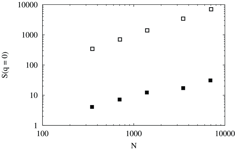
FIG. 5.: Density fluctuation of randomly distributed $(\square)$ and pre-packed Gaussian chains $(\vrule height=3.87495pt,width=3.44444pt,depth=-0.43057pt)$ for various chain lengths. By pre-packing the density fluctuations are about 1% for $N=350$ and 0.5% for $N=7000$ of that for randomly distributed chains.

FIG. 6.: Mean square internal distances for pre-packed systems after a (a) fast push-off and (b) slow push-off for chains with $k_{\theta}=0$. Symbols as in Fig.  3. The thick line is our target function from Fig. 2.

B Slow push-off

In order to further reduce the chain deformations we have modified the push-off procedure in three ways:

1. Replace the cos-potential Eq. (3) with a force-capped-Lennard-Jones-potential, [21].

2. Keep the full excluded volume between next-nearest neighbor monomers to preserve to non-reversal-random-walk structure (see sec. III).

3. Increase the push-off time.

Force-capping [21] can either be defined directly via a maximum force $F_{\mathrm{m}ax}$ or implicitly via a distance $r_{fc}$ where ${\rm U_{LJ}}^{\prime}(r_{fc})\equiv F_{\mathrm{m}ax}$. At larger separations, the interaction is defined by Eq. (1), at smaller distances the force becomes constant so that the interaction potential grows only linearly with $(r-r_{fc})$:

$${\rm U_{FCLJ}}(r)=\left\{\begin{array}[]{cc}(r-r_{fc})*{\rm U_{LJ}}^{\prime}(r_{fc})+{\rm U_{LJ}}(r_{fc})&r<r_{fc}\\ {\rm U_{LJ}}(r)&r\geq r_{fc}\end{array}\right.$$

In the present case, $r_{fc}$ is gradually reduced from the Lennard-Jones cut-off radius $r_{c}=2^{1/6}\sigma$ to $0.8\sigma$ which is significantly smaller than the relevant interparticle distances.

Force-capping has the advantage that the soft potential systematically approaches the true potential. In contrast, the cos-potential overcompensates the missing singularity at the origin by a fast rise of the repulsive interactions close to the cut-off distance. This leads to slight differences in the monomer packing. As a result, the chain conformations are slightly perturbed after switching to the full LJ-potential.

We have increased the push-off time in order to introduce the excluded volume interactions quasi-statically. In practice, one has in this context to worry about two issues: (i) How slow is slow enough? (ii) What is the equilibrium statistics for polymers with force-capped interactions? Concerning the first point, we have chosen a push-off time of $5000\tau$, which is of the order $\tau_{\rm Rouse}(50)$. This covers the typical subchain regime, up to which the intrachain distances still were disturbed by a fast push-off. The second question is more difficult to answer. If we simply switch off the repulsive monomer-monomer interaction, we find $\left<R^{2}\right>=0.94\sigma^{2}N$, while the effective stiffness $c_{\infty}\approx 1.7$ of our chains in the melt is due to local bead packing effects. Thus a slow push off starting from a potential for which the end-to-end distance is an ideal random walk is also dangerous. For bead-spring chains these effects can easily be accounted for by treating the chains as NRRWs by always keeping the full LJ excluded volume between next-nearest neighbors along the chain. For atomistic polymer models, it is necessary to extend this to larger distances along the chain (“pentane effect”).[21] Once this adjustement is made the push off procedure cannot be “too slow”and the chain size varies only very weakly with the maximum excluded volume force.

Figure 6b shows that the new procedure works quite well. Independent of the total chain length $N$ the chains are no longer stretched on intermediate scales and the large scales remain unaffected by the introduction of excluded volume interactions. As an additional check, we have varied the stiffness of the initially generated random walks over a range of about 20% (Fig. 7a). Fig. 7b compares the internal distances after pre-packing and slow push-off and confirms our previous observations. The chains are fully equilibrated on short scales, where the results are independent of the initial conditions. In contrast, internal distances beyond $n=100$ remain practically unaffected. We therefore conclude that our new method allows the preparation of well-equilibrated melts of extremely long chains within reasonable computational effort, provided the correct asymptotic chain stiffness $c_{\infty}$ is known from a careful extrapolation of simulation results for well-equilibrated short and medium chain length melts. For our largest system of $M=80$ chains of length $N=7000$, an equilibration time of $5000\tau$ takes about one month on a single processor or about 8 hours on the 100 processor DEC alpha cluster. Thus even with moderate computational means it is possible to equilibrate very large systems using a combined pre-packing and slow push-off procedure.

FIG. 7.: Influence of the effective stiffness used to generate the initial sets of random walks on the final configurations for systems with $k_{\theta}=0$. The figure shows mean square internal distances (a) before and (b) after pre-packing and slow push-off. From top to bottom the curves represent results for chains with length $N=3500$ which were set up with a stiffness varying by $-4\%,\ -2\%,\ 0\%,\ +2\%,\ +4\%,\ +6\%,\ +8\%,\ +10\%$ and $+12\%$ relative to our initial guess of $c_{\infty}=1.7$. The thick line is our target function from Fig. 2.

VII Double-Pivot-MD Hybrid Algorithm

The present section deals with the problem of accelarating the dynamic equilibration of a long chain polymer melt. We describe a double-pivot-MD hybrid algorithm which performs this task significantly faster than simple MD relaxation. In contrast to the methods discussed in the previous section, the dynamic equilibration of a dense polymer melt does not require independent knowledge of the effective $c_{\infty}$. However, the preparation of locally equilibrated samples can significantly reduce the required relaxation times.

In the original pivot algorithm[11, 12, 13, 14] one choses a monomer at random and one of the two segments formed by that partitioning is pivoted rigidly in a random direction about the selected monomer. The pivot algorithm is extremely efficient when applied to isolated chains in an implicit solvent. However, in a melt or even in a solution at moderate density, pivot moves applied to a single chain are bound to be rejected, since they lead to strong excluded volume interactions with other chains.

An attractive alternative are Monte Carlo moves involving at least two chains, which change the connectivity within the melt in a way that the overall packing of beads remains (almost) unaffected. Such algorithms were first introduced for lattice models[30, 31] and recently extended to off-lattice models.[2, 10, 16, 17, 18] The efficient equilibration usually comes at the expense of a certain amount of polydispersity which is introduced into the samples, though recently Karayiannis[17, 18] have overcome this limitation using double-bridging Monte Carlo moves. For the bead-spring polymers studied here, the algorithm is straightforward to implement since the bond length $l$ is comparable to the excluded volume parameter $\sigma$. This certainly is a unique situation, as for many bead spring coarse grained models of specific chemical species, the above ratio is not as close to one. For example in the case of a united atom model for polyethylene where the bond length $l=1.54\AA$ is significantly smaller then $\sigma\approx 4.0\AA$, it is necessary to construct two trimer bridges between the two properly chosen dimers along the backbone.[17, 18] For the bead spring model studied here, complex bridging moves are not necessary. For this reason we refer to the method as the double-pivot algorithm since it is much closer to the pivot algorithm used for single chains in an implict, continuum solvent.

In order to maintain a monodisperse melt we search for a pair of spatial neighbor monomers $i$ and $j$ on different chains or on the same chain, which happen to also be the same distance from one end of their respective chain. Then one can replace two bonds along the original chains with two new bonds or bridges across the pair of chains. The total change in energy $\Delta E$ is local and consists of the sum of the energies of the two new bonds minus the energies of the two previous bonds as well as the difference in the bending energy, which involves the sum of the energies of four new angles minus the energies of the four previous angles for the case $k_{\theta}\neq 0$. The move is accepted by a standard Metropolis criterion, namely with a Boltzmann weight $\exp{(-\Delta E/k_{B}T)}$ if $\Delta E>0$ and $1$ if $\Delta E\leq 0$. As in the original pivot algorithm, the double-pivot algorithm generates new chains which are substantially different from the original two chains since as many as $N/2$ monomers of a chain are replaced by monomers from the other chain. This results in immediate large changes in the end-to-end distance and radius of gyration.

We have implemented the double-pivot algorithm into both our shared memory and distributed memory MD codes. The details of the implementation and a discussion of its computational efficiency will be published elsewhere. Briefly in our shared memory code, every $3-5$ time steps, we randomly chose a monomer $i$ and check its non-bonded nearest neighbors to determine if any satisfy the condition that they are equidistant from the end of their chain. If so, the energy change $\Delta E$ of the double-pivot move is determined and the move accepted or rejected on the basis of the Metropolis criterion. If the move is accepted, monomers and/or the connectivity table are re-labeled depending on which of the two codes is used and the MD simulation is continued. If the move is rejected or no suitable pair is identified, a new monomer is chosen at random and the process repeated. If no suitable pair is generated after searching a specified fraction of monomers (usually $2-5\%$ depending on the chain length $N$), we continue with the MD simulations for another $3-5$ steps and repeat the procedure. On the distributed memory code, the procedure is similar except that each processor randomly choses a monomer $i$ and checks its non-bonded nearest neighbors on the same processor to see if they satisfy the condition that they are equidistant from the end of their chain. If no suitable non-bonded neighbor is found, another monomer $i$ is randomly selected. The process is continued until a specified fraction of the momomers, typically 50%, are tested. To facilitate determining the distance from the free end, each chain carries an extra label starting from $1$ at either end to $N/2$ at the center. Because each processor searches a unique region of space independently, it is possible to have multiple successful moves each time the procedure is applied. The search is restricted to sets of monomers on the same processor to avoid the need to communicate changes in chain topologies between processors. This restriction also prevents two or more processors from performing simultaneous swaps that could energetically conflict with each other. While this restriction means (slightly) less swaps are considered, this is more than outweighed by the parallelism, e.g. up to $P$ swaps take place in one time step, where $P$ is the number of processors. With the standard parameters of the FENE potential, $k=30\epsilon/\sigma^{2}$, the acceptance rate is quite low. A way to improve the acceptance rate is to start with a somewhat lower value, $k=10-15\epsilon/\sigma^{2}$ and gradually increase $k$ during the course of the simulation. This change has little effect on the overall structure of the chains but increases significantly the acceptance rate. Using our distributed memory code on 27 DEC alpha processors for a system of $M=500$ chains of length $N=500$, the number of successful exchanges for $10^{5}\Delta t$ with $k_{\theta}=0$ was approximately $1750$ for $k=30\epsilon/\sigma^{2}$ compared to $8500$ for $k=20\epsilon/\sigma^{2}$ and $49500$ for $k=10\epsilon/\sigma^{2}$.

To demonstrate the effectiveness of the double-pivot algorithm, we have applied it to a melt of $M=500$ chains of length $N=500$ generated using the standard fast push-off procedure outlined in Sec. V. Figure 8 shows the internal distances as a function of time during a double-pivot/MD relaxation. Note that the characteristic “bump” in the internal distance function does not simply decay. Rather, Figure 8 shows that the (seemingly equilibrated) largest scales are first swollen, before the chain dimensions decay homogeneously on all scales. Equilibration for the reduced spring constant $k=10\epsilon/\sigma^{2}$ was achieved after about $6\times 10^{4}\tau$ or 10 accepted pivot moves per monomer. The penalty for reducing the spring constant to $k=10$ is an increase of the mean-square bond length by $7\%$, while the chain stiffness $c_{\infty}$ remains unaffected. In subsequent runs, the spring constant $k$ is increased to slowly “reel in” in the chains. This required an additional $6\times 10^{4}\tau$. We made no attempt to optimize the number of steps for each value of $k$. Nevertheless, the required equilibration times are considerably shorter than the time $\tau_{max}(500)\approx 4\times 10^{6}\tau$ for the chains to move their own size in a pure MD simulation.

These observations illustrate the close analogy between the pivot algorithm for single chains and the double-pivot algorithm for dense polymer melts. As pointed out by Madras and Sokal[13], it is useful to distinguish between decorrelation and equilibration in discussing the performance of such algorithms. Pivoting is extremely efficient in decorrelating large length scales, provided the initial conformation is properly equilibrated. Up to small corrections, the number of pivot moves needed to decorrelate the end-to-end distance of isolated chains in an implicit solvent is ${\cal O}(10)$ independent of chain length. Since the same holds for subchains of arbitrary length, correspondingly more moves are required to decorrelate higher order (Rouse) modes. In other words, the decorrelation proceeds from large to small scales. However, the same is not correct for the equilibration of a perturbed initial configuration. In this case it is necessary to run the system up to the decorrelation time of the shortest perturbed length scale in order to equilibrate the chains on all length scales. For single chain studies aiming at global properties Madras and Sokal [13] therefore recommend to apply the pivot algorithm to equilibrated initial configurations generated by other techniques. In the present case, the combination of pre-packing with a slow push-off at least partially fulfills these requirements, since the chains are locally equilibrated.

Since equilibration requires that each monomer comes close enough to suitable exchange partners, one may ask whether of ${\cal O}(10)$ exchanges per monomer independent of $N$ is sufficient or whether the exchanges are simply being made back and forth between a limited number of states. To estimate whether enough independent configurations are being sampled, consider the time for a monomer to diffusive a typical distance between monomers with the same index $(\rho/(N/2))^{-1/3}$ between successful pivot moves. If we assume that monomers diffuse with the typical $\langle\delta r^{2}\rangle=\sqrt{k_{B}Tb^{2}t/\zeta}$ Rouse dynamics, this corresponds to

$$t_{piv}=\left(\frac{(N/2)}{\rho}\right)^{4/3}\frac{\zeta}{k_{B}Tb^{2}}$$ (9)

which is equivalent to the Rouse time of a chain of length $N_{eff}=(N/2)^{2/3}$. For our longest chains $N=7000$, $N_{eff}\approx 236$. The Rouse time for a chain of length $N=236$ is approximately $7\times 10^{4}\tau$, which is still much less than the time needed to make ${\cal O}(10)$ exchanges per monomer even if we used the reduced spring constant $k=10$. Thus only for much longer chains or more complex architectures does one have to worry about sufficient independent configurations being sampled by this hybrid double-pivot-MD algorithm.

FIG. 8.: Equilibration of mean square internal distances using combined double-pivot-MD relaxation following a fast push-off for 500 chains of length $N=500$. Results for $t=0\ (+)$ just after the push-off, $6\times 10^{3}\tau\ (\times)$, $1.2\times 10^{3}\tau\ (*)$, $6\times 10^{4}\tau\ (\square)$ and $1.2\times 10^{5}\tau\ (\vrule height=3.87495pt,width=3.44444pt,depth=-0.43057pt)$. In order to increase the acceptance rate of the pivot moves we used a reduced spring constant $k=10\epsilon/\sigma^{2}$ for $0<t<6\times 10^{4}\tau$ and $k=20\epsilon/\sigma^{2}$ for $6\times 10^{4}\tau<t<9.6\times 10^{4}\tau$ before switching to $k=30\epsilon/\sigma^{2}$ for $9.6\times 10^{4}\tau<t<1.2\times 10^{5}\tau$.

VIII Local bending rigidity

As a last point we present results for chains with intrinsic stiffness Eq. (2). In section IV we referred to this case as a “blind test,” because the starting states were generated based on our simple estimate Eq. (7) for the effective chain stiffness in the melt and before the brute-force MD runs for the target functions shown in Fig. 2 were completed. As can be seen in Fig. 1, our original estimates were slightly too large. A comparison with the target functions after the pre-packing and slow push-off phase (Fig. 9a) shows that as for fully flexible chains the correct chain statistics is reproduced on short length scales. However, we are now in a situation comparable to the situtaion presented in Fig. 7 where the large length scales are not fully equilibrated, because the initial chains were generated with a slightly incorrect effective stiffness.

	$k=10$	$k=20$	$k=30$
$k_{\theta}=0.0$	24800	3900	840
$k_{\theta}=0.75$	27000	4200	894
$k_{\theta}=1.5$	21200	3500	770
$k_{\theta}=2.0$	15500	2700	600

TABLE II.: Influence of the strength of the FENE spring constant $k$ on the number of successful double-pivot exchanges per $10^{5}$ time steps for a system of 200 chains of length $N=350$ on 27 DEC alpha processors.

Subsequently, we ran the combined double-pivot-MD simulation for $1.08\times 10^{5}\tau$ with $k=10$ for the first 4 millions steps, $k=20$ for the second $4$ million steps and $k=30$ for the last million steps for a system of $200$ chains of $N=350$ for $k_{\theta}=1.5$ and $2.0$ and $N=700$ for $k_{\theta}=0.75$. The resulting mean squared end-to-end distance were in excellent agreement with the target functions generated by brute force MD simulations for shorter chains. Table II shows an example of the number of successful exchanges per $10^{5}$ steps for the system of $200$ chains of length $N=350$ monomers for three values of the spring constant $k$ for four values of $k_{\theta}$ for our distributed memory code run on 27 DEC alpha processors. As seen from this table, the procedure used gives approximately $9-12$ successful exchanges for $k=10$, $2$ successful exhanges for $k=10$ and $0.1$ for $k=30$. Fortunately there is little difference in the local structure of the chain for $k=20$ compared to $k=30$, though as seen from Fig. 8, the chain is expanded for $k=10$. Thus there is a definite tradeoff between reducing the bond spring constant $k$, which increases the number of exchanges while at the same time increasing the mean squared bond length. Note that for longer chains lengths, the length of the run and/or the number of processors would have to be increased so that the number of successful exchanges is on the order of ${\cal O}(10)$. This limits the double-pivot/MD hydrid method to moderate chain lengths.

FIG. 9.: Mean square internal distances for chains with local bending rigidity (a) after pre-packing and slow push-off and (b) after an additional double-pivot-MD relaxation of length $1.08\times 10^{5}\tau$. Results for $k_{\theta}=0\ (*)$, $0.75\epsilon\ (+)$, $1.5\epsilon\ (\times)$, and $2.0\epsilon\ (\square)$. We did not apply the additional double-pivot-MD relaxation to our fully flexible systems, which are well-equilibrated after pre-packing and slow push-off. The thick lines are our target functions from Fig. 2 which were generated a posteriori for chains with intrinsic stiffness.

IX Conclusions

In this paper, we have discussed the preparation of equilibrated melts of long chain polymers in computer simulations. The interest in reliable algorithms for this task is due to two problems: (i) the prohibitively long relaxation times encountered in brute force MD simulations and (ii) the difficulty to predict the chain statistics on large scales (i.e. the effective chain stiffness $c_{\infty}$) on the basis of microscopic intra- and interchain interactions.

Our results can be summarized as follows:

• It is insufficient to judge the quality of the equilibration from the statistics of the chain end-to-end distances or radius of gyration. The first just measures one length, while the latter gives a non specific average over all internal distances. As a much more sensitive criterion we measure mean square internal distances on all length scales from the monomer size up to the contour length of the chains.

• Our standard method to rapidly introduce excluded volume interactions between randomly assembled Gaussian chains with the correct overall statistics (“fast push-off”) fails, when judged according to this improved criterion. The fast push-off introduces significant chain distortions on length scales of the order of the tube diameter. They can only vanish when the local melt topology is equilibrated. In MD simulations this is only possible via reptation dynamics so that the proper equilibration requires runs whose length exceeds the disentanglement time of the chains. To overcome this problem we have introduced two different methods.

• We have modified our standard approach by reducing the density fluctuations in the assembly of Gaussian chains (“pre-packing”) and by introducing the excluded volume interactions in a quasi-static manner (“slow push-off”). As before, this method requires prior knowledge of $c_{\infty}$. Tests for bead-spring models with chain lengths up to $N=7000$ $(N/N_{e}={\cal O}(100))$ show that suitable push-off times are the Rouse times of the characteristic chain lengths of the overshoot. In the present case this time is of the order of a few entanglement times, independent of $N$.

• We have applied a “double-pivot” algorithm which is inspired by the highly efficient pivot algorithm for single chains and the double-bridging method for dense systems. For intermediate chain lengths, this is a viable method to equilibrate melts in a reasonable amount of cpu time, particularly when one has no prior knowledge of $c_{\infty}$.

The combination of MD relaxation, double-pivot and slow push-off allows the efficient and controlled preparation of equilibrated melts of short, medium and long chains respectively. While our results were obtained for an off-lattice bead spring model with chain lengths up to $N=7000$ beads, the methods should work as efficiently for lattice polymer models such as the bond fluctuation model.[32, 33] The pre-packing and gradual introduction of the excluded volume are also applicable to united and explicit atom simulations. Furthermore, the methods are applicable to polydisperse melts and to branched polymers, including long chain branching, comb and star polymers. The double-pivot and double bridging algorithms has also been used to equilibrate long end-tethered, polymer brushes in contact with a melt of long chains.[18, 34] For these more complex chain architectures, in which the chains are not necessarily Gaussian and there is no a priori way to know the conformation of the chains, algorithms like the double-pivot and double-bridging algorithms are presently the only possible way to equilibrate systems faster than extremely long MD or MC runs.

REFERENCES

- [1] W. Paul et al., Phys. Rev. Lett. 80, 2346 (1998).
- [2] V. G. Mavrantzas, T. D. Boone, E. Zervopoulou, and D. N. Theodorou, Macromolecules 32, 5072 (1999).
- [3] M. Pütz, K. Kremer, and G. S. Grest, Europhys. Lett. 49, 735 (2000).
- [4] A. Bunker and B. Dünweg, Phys. Rev. E 63, 016701 (2001).
- [5] M. Vacatello, G. Avitabile, P. Corradini, and A. Tuzi, J. Chem. Phys. 73, 548 (1980).
- [6] J. J. dePablo, M. Laso, and U. W. Suter, J. Chem. Phys. 96, 2395 (1992).
- [7] J. I. Siepmann and D. Frenkel, Molec. Phys. 75, 59 (1992).
- [8] L. R. Dodd and D. N. Theodorou, Adv. Polym. Sci. 116, 249 (1994).
- [9] L. R. Dodd, T. D. Boone, and D. N. Theodorou, Molec. Phys. 78, 961 (1993).
- [10] P. V. K. Pant and D. N. Theodorou, Macromolecules 28, 7224 (1995).
- [11] M. Lal, Mol. Phys. 17, 57 (1969).
- [12] B. MacDonald, J. Phys. A 18, 2627 (1985).
- [13] N. Madras and A. D. Sokal, J. Stat. Phys. 50, 109 (1988).
- [14] B. Li, N. Madras, and A. D. Sokal, J. Stat. Phys. 80, 661 (1995).
- [15] W. W. Graessley, R. C. Hayward, and G. S. Grest, Macromolecules 32, 3510 (1999).
- [16] A. Uhlherr, V. G. Mavrantzas, M. Doxastakis, and D. N. Theodorou, Macromolecules 34, 8554 (2001).
- [17] N. C. Karayiannis, V. G. Mavrantzas, and D. N. Theodorou, Phys. Rev. Lett. 88, 105503 (2002).
- [18] N. C. Karayiannis, A. E. Giannousaki, V. G. Mavrantzas, and D. N. Theodorou, J. Chem. Phys. 117, 5465 (2002).
- [19] K. Kremer and G. S. Grest, J. Chem. Phys. 92, 5057 (1990).
- [20] A. Yethiraj and C. K. Hall, Macromolecules 23, 1865 (1990).
- [21] D. Brown, J. H. R. Clarke, M. Okuda, and T. Yamazaki, J. Chem. Phys. 100, 6011 (1994).
- [22] J. Gao, J. Chem. Phys. 102, 1074 (1995).
- [23] M. Mondello, G. S. Grest, E. B. Webb III, and P. Peczak, J. Chem. Phys. 109, 798 (1998).
- [24] M. Kröger, Comp. Phys. Comm. 118, 278 (1999).
- [25] K. Kremer and G. S. Grest, in Monte Carlo and Molecular Dynamics Simulations in Polymer Science, edited by K. Binder (Oxford University Press, New York, 1995), p. 194.
- [26] B. Dünweg, G. S. Grest, and K. Kremer, in Numerical Methods for Polymeric Systems, edited by S. G. Whittington (Springer-Verlag, New York, 1998), Vol. 102, p. 159.
- [27] C. F. Abrams and K. Kremer, J. Chem. Phys. 116, 3162 (2002).
- [28] J. S. Shaffer, J. Chem. Phys. 103, 761 (1995).
- [29] J. S. Shaffer, Macromolecules 29, 1010 (1996).
- [30] M. L. Mansfield, J. Chem. Phys. 77, 1554 (1922).
- [31] O. F. Olaj and W. Lantschbauer, Makromol. Chem. Rapid Comm. 3, 847 (1982).
- [32] I. Carmesin and K. Kremer, Macromolecules 21, 2819 (1988).
- [33] H.-P. Deutsch and K. Binder, J. Chem. Phys. 94, 2294 (1991).
- [34] S. W. Sides, G. S. Grest, M. J. Stevens, and S. J. Plimpton, unpublished (2003).