Multifractality of Hamiltonians with power-law transfer terms

Abstract

Finite-size effects in the generalized fractal dimensions $d_{q}$ are investigated numerically. We concentrate on a one-dimensional disordered model with long-range random hopping amplitudes in both the strong- and the weak-coupling regime. At the macroscopic limit, a linear dependence of $d_{q}$ on $q$ is found in both regimes for values of $q\lesssim 4g^{-1}$, where $g$ is the coupling constant of the model.

I Introduction

Quantum phase transitions in disordered electronic systems remain one of the central problems in condensed-matter physics. Considerable attention has recently focused on the critical eigenfunctions, which strongly fluctuate near the critical point and thus have multifractal scaling properties.HP83 ; Ja94 ; FE95 ; Mi00 ; CO02 Wave-function statistics can be characterized through the set of generalized fractal dimensions $d_{q}$ which are associated with the scaling of the $q$th moment of the wave-function intensity. A complete knowledge of $d_{q}$ is equivalent to a complete physical characterization of the fractal.HP83

Metal-insulator transitions (MIT’s) depend on the dimensionality and symmetries of the system and can occur in both the strong disorder and the weak disorder regime (strong-coupling or weak-coupling regime, respectively, of the corresponding field-theoretical description). Each regime is characterized by its respective coupling strength $g$, which depends on the ratio between diagonal disorder and the off-diagonal transition matrix elements of the Hamiltonian.Ef83

For a multifractal structure of wave functions, the $q$ dependence of the fractal dimensions $d_{q}$ is given by the linear relation

$$d_{q}=d-c_{g}q\;,\quad q\lesssim b\;,$$ (1)

where $c_{g}\ll 1$ and $b$ are parameters related to the coupling constant of the corresponding model (see below). This equation has been obtained for different transitions in the weak-coupling limit using different approaches, which we summarize in the following paragraphs. Equation (1) describes weak multifractality in the sense that the fractal dimensions $d_{q}$ slightly deviate from the system dimensionality $d$ characteristic of the homogeneously spread metallic wave functions.

In the context of the theory of Anderson localization, Eq. (1) was obtained,FE95 in the leading order in $1/2\pi\nu D\ll 1$, for two-dimensional (2D) conductors on the basis of a reduced version of the supersymmetric $\sigma$ model. In this case $c_{g}=1/2\pi^{2}\nu\beta D$, where $\nu$ is the density of states, $D$ the diffusion constant, and $\beta$ the symmetry parameter.

Using a perturbative $\epsilon$ expansion in one-loop order for a $d=2+\epsilon$ dimensional system, Eq. (1) was found,We80 in the leading order in $\epsilon\ll 1$, with $c_{g}=\epsilon$. This derivation was made for the case of unbroken time-reversal symmetry (orthogonal universality class) in the weak-coupling limit.

Reference 8 derived Eq. (1) with $c_{g}=g/8\pi$, in the limit $g\ll 1$ for the power-law random banded matrix model (orthogonal universality class). This solution was found by mapping the problem onto a nonlinear $\sigma$ model with nonlocal interaction.

Equation (1) was also obtained, using the replica trick,LF94 for the critical wave function of a 2D Dirac fermion in a random vector potential (chiral universality class). The $c_{g}=\Delta_{A}/\pi$ found depends on the variance $\Delta_{A}$ of the Gaussian distributed vector potential. This result was confirmed recently MC96 ; CD01 by mapping the problem to a Gaussian field theory in an ultrametric space.

Field-theoretical approaches in the context of the integer quantum Hall transition (unitary universality class) have been addressed recently. Based on the application of conformal field theory to the critical point of a 2D Euclidean field theory, Bhaseen et al. BK00 derived Eq. (1) with $c_{g}=2/k$, where $k$ is the inverse coupling constant.

We wish to point out that the existing theories are inherently weak-coupling results. However, MIT’s generically take place at strong disorder, where the energy scales associated with both disorder and interactions are comparable to the Fermi energy, unlike to what happens in perturbative $2+\epsilon$ expansion approaches or in effective-field theories. Thus, quantitative results for $d_{q}$ are lacking at strong coupling, and finding $d_{q}$ for this regime is essential in order to fully understand the MIT’s.

The aim of this work was twofold. First, a numerical verification of the weak-coupling phase result, Eq. (1). Second, and most importantly, we were interested in finding the $q$ dependence of $d_{q}$ in the strong-coupling regime, which has been left unexplored. Since this case is not accessible by the previous treatments, the problem can only be addressed by using numerical calculations.

The paper begins by first giving the model and the methods used for the calculations in Sec. II. The results for the fractal dimensions in the weak- and the strong-coupling regimes are presented in Sec. III A and III B, respectively. Finally, Sec. IV summarizes our findings.

II Model and methods

The disorder-induced MIT is usually investigated for Hamiltonians with short-range, off-diagonal matrix elements (e.g., the canonical Anderson model). Other Hamiltonians exhibiting a MIT in arbitrary dimension $d$ are those that include long-range hopping terms.PS98 ; PS02 The effect of long-range hopping on localization was originally considered by Anderson An58 for randomly distributed impurities in $d$ dimensions with the $V(\bm{r}-\bm{r^{\prime}})\sim|\bm{r}-\bm{r^{\prime}}|^{-\alpha}$ hopping interaction. It is known An58 ; Le89 that all states are extended for $\alpha<d$, whereas for $\alpha>d$ the states are localized. Thus, the MIT can be studied by varying the exponent $\alpha$ at fixed disorder strength. At the transition line $\alpha=d$, a real-space renormalization group can be constructed for the distribution of couplings.Le89 ; Le99 These models are the most convenient for studying critical properties numerically since the exact quantum critical point is known ($\alpha=d$) and, in addition, they allow the 1D case to be treated, thus using larger system sizes and reducing the numerical effort. Many real systems of interest can be described by these Hamiltonians. Among such systems are optical phonons in disordered dielectric materials coupled by electric dipole forces,Yu89 excitations in two-level systems in glasses interacting via elastic strain,BL82 magnetic impurities in metals coupled by an $r^{-3}$ Ruderman-Kittel-Kasuya-Yodida interaction,CB93 and impurity quasiparticle states in 2D disordered $d$-wave superconductors.BS96

We will consider here the intensively studied power-law random banded matrix model (PRBM) Mi00 ; ME00 ; MF96 ; CG01 ; CO02 ; Va02 ; Cu02 ; KM97 ; KT00 . The corresponding Hamiltonian, which describes a disordered 1D sample with random long-range hopping, is represented by real symmetric matrices, whose entries are randomly drawn from a normal distribution with zero mean, $\left\langle{\cal H}_{ij}\right\rangle=0$, and a variance which depends on the distance between the lattice sites,

$$\left\langle|{\cal H}_{ij}|^{2}\right\rangle=\frac{1}{1+(|i-j|/b)^{2}}\times\left\{\begin{array}[]{ll}\tfrac{1}{2}\ ,&i\neq j\\ 1\;\;\;\,\ ,&i=j\;,\end{array}\right.$$ (2)

where the parameter $b$ plays the role of the inverse coupling constant $b=4g^{-1}$ of the corresponding $\sigma$ model at the center of the spectral band. The model describes a whole family of critical theories parametrized by $0<b<\infty$, which determines the critical dimensionless conductance, in the same way as the dimensionality labels the different Anderson transitions. In the two limiting cases $b\gg 1$ and $b\ll 1$, which correspond to the weak and the strong disorder limits, respectively, some critical properties have been derived analytically. Mi00 ; ME00 ; KM97 ; MF96 ; KT00 More specifically, as already mentioned in the Introduction, in Ref. 8 the following equation in the limit $b\gg 1$ was derived,

$$d_{q}=1-\frac{q}{2\pi b}\;,\quad q\ll 2\pi b\;.$$ (3)

The system size ranges between $L=180$ and $L=5400$, and $0.01\leq b\leq 12$. We restrict ourselves to values of $q\lesssim b$, and consider a small energy window, containing about 5% of the states around the center of the band. The number of random realizations is such that the number of critical states included for each $L$ is roughly $4\times 10^{5}$, while, in order to reduce edge effects, periodic boundary conditions are included. Using methods based on level statistics, we checked that the normalized nearest level variances Cu99 are indeed scale invariant at each critical point studied.

For the computation of $d_{q}$ we used the standard box-counting procedure, Ja94 first dividing the system of $L$ sites into $N_{l}=L/l$ boxes of linear size $l$ and determining the box probability of the wave function in the $i$ box by $p_{i}(l)=\sum_{n}|\psi_{kn}|^{2}$, where the summation is restricted to sites within that box, and $\psi_{kn}$ denotes the amplitude of an eigenstate with energy $E_{k}$ at site $n$. The normalized $q$th moments of this probability constitute a measure. From this, the mass exponents $\tau_{q}(L)$, which encode generalized dimensions $d_{q}(L)=\tau_{q}(L)/(q-1)$, can be obtained,CJ89

$$\tau_{q}(L)=\lim_{\delta\to 0}\frac{\ln\sum_{i=1}^{N_{l}}p_{i}^{q}(l)}{\ln\delta}\;,$$ (4)

where $\delta=l/L$ denotes the ratio of the box sizes and the system size. It should be made clear that the calculation of $\tau_{q}(L)$ is suitable only if the conditions Ja94

$$a\ll l<L\ll\xi\$$ (5)

are satisfied, where $\xi$ is the localization or correlation length and $a$ is the lattice spacing (or any microscopic length scale of the system). In practice, $\tau_{q}(L)$ is found by performing a linear regression of $\ln\sum_{i=1}^{N_{l}}p_{i}^{q}(l)$ with $\ln\delta$ in a finite interval of $\delta$ (usually $a/L\leq\delta\leq 1/2$). In order to properly satisfy the previous conditions (5) and (4), in this work we will compute the derivative

$$\tau_{q}(L)=\frac{\textit{d}\ln\sum_{i=1}^{N_{l}}p_{i}^{q}(l)}{\textit{d}\ln\delta}\biggr{|}_{\delta=0.1}\;.$$ (6)

First, $\tau_{q}(L)$ was calculated for different system sizes and then extrapolated to the macroscopic limit $\tau_{q}=\lim_{L\to\infty}\tau_{q}(L)$.

III Results

III.1 Weak-coupling regime ($b\gg 1$)

Using the exact eigenstates of Hamiltonian (2) obtained from numerical diagonalizations, we evaluate, for each value of $q$, $L$, and $b$, the numerator on the right-hand side of Eq. (4) for decreasing box sizes, and then calculate $\tau_{q}(L)$ from the slope of the graph of the numerator vs $\ln\delta$ at $\delta=0.1$, Eq. (6). Fig. 1 provides an example of the $\ln\delta$ dependence of $\ln\sum_{i=1}^{N_{l}}p_{i}^{q}(l)$ in the weak-coupling regime ($b=10$) for a system size $L=5400$ and different values of $q$: $4$ (circles), 5 (triangles), 6 (diamonds), and 7 (squares); the dotted vertical line corresponds to $\delta=0.1$. The inset shows the same dependence of the corresponding slopes, $\textit{d}\ln\sum_{i=1}^{N_{l}}p_{i}^{q}(l)/\textit{d}\ln\delta$. Note that these derivatives are practically constant in the region shown. We have checked that the results were practically the same when $\tau_{q}(L)$ was obtained from the linear fit to $\ln\sum_{i=1}^{N_{l}}p_{i}^{q}(l)$ vs $\ln\delta$ in the interval $0.1\lesssim\delta\lesssim 0.4$.

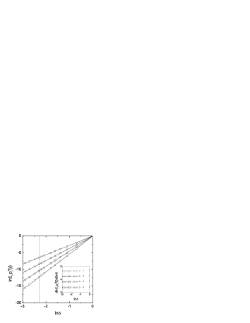
Figure 1: The $\ln\delta$ dependence of $\ln\sum_{i=1}^{N_{l}}p_{i}^{q}(l)$ in the weak-coupling regime ($b=10$) for $L=5400$ and different $q$ values: $q=4$ (circles), 5 (triangles), 6 (diamonds), and 7 (squares); the dotted vertical line corresponds to $\delta=0.1$. The inset shows the same dependence of corresponding slopes, $\textit{d}\ln\sum_{i=1}^{N_{l}}p_{i}^{q}(l)/\textit{d}\ln\delta$.

The size dependence of $\tau_{q}(L)$ at the critical point of the finite system for $b=10$ is shown in Fig. 2 for $q=4$. Clearly, significant finite-size effects are present, and for the larger values of $L$ the convergence is evident. In order to predict the asymptotic value of $\tau_{q}$ from such a plot, a curve of the form $\tau_{q}(L)=\tau_{q}+F_{a_{q},c_{q}}(L)$ was fitted to the data points in this graph, where $\tau_{q}$, $a_{q}$, and $c_{q}$ are three fitting parameters and $F_{a_{q},c_{q}}(L)$ is a function which tends to zero as $L\to\infty$. Various forms for $F_{a_{q},c_{q}}(L)$ were chosen and tested on the data plots, including exponential ($\sim e^{-c_{q}L}$), inverse logarithmic ($\sim 1/\ln c_{q}L$), and power-law ($\sim L^{-c_{q}}$) decay with $L$. The testing involved performing a three-parameter fit on the $\tau_{q}(L)$ vs $L$ data plots using the standard Levenberg-Marquardt method for nonlinear fits. The form of $F_{a_{q},c_{q}}(L)$ eventually chosen was the power law. The reason for choosing the above form with preference to the alternative forms was simply that the inverse logarithmic and the exponential laws did not fit our data properly. In addition, for all values of $q$ and $b$ we found that the exponent $c_{q}$ hardly differs from unity. Thus, we can write

$$\tau_{q}(L)=\tau_{q}+a_{q}/L\;,$$ (7)

and keep only two free parameters. The solid line in Fig. 2 is a fit to Eq. (7). Note that this equation gives a fairly good fit to the data. $\tau_{q}(L)$ is represented on a $1/L$ scale in the inset of Fig. 2 for different values of $q$: $4$ (circles), 5 (triangles), 6 (diamonds), and 7 (squares). Here, one can better appreciate the linear behavior, Eq. (7), of the finite-size corrections to $\tau_{q}$.

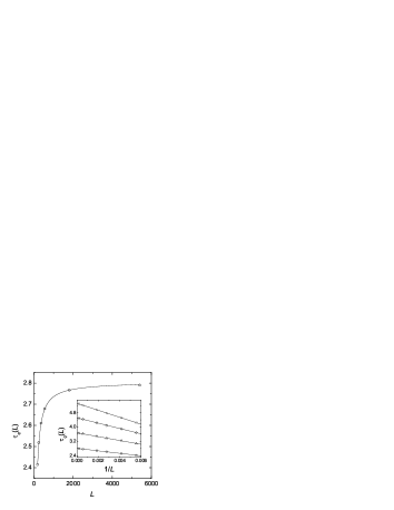
Figure 2: The $L$ dependence of the mass exponent $\tau_{q}(L)$ in the weak-coupling regime ($b=10$) for $q=4$ (circles); solid line is a fit to Eq. (7). The inset shows $\tau_{q}(L)$ on a $1/L$ scale for different $q$ values: $q=4$ (circles), 5 (triangles), 6 (diamonds), and 7 (squares); the straight lines are linear fits to Eq. (7).

The $q$ dependence of the extrapolated results of $d_{q}=\tau_{q}/(q-1)$ in the weak-coupling regime are depicted in the inset of Fig. 3 for several values of $b$: $6$ (squares), $8$ (triangles), $10$ (diamonds), and $12$ (circles). The solid lines are fits to the form $d_{q}=1-c_{b}q$. The corresponding $b$-dependent slopes $c_{b}$ are summarized and compared with the nonlinear $\sigma$-model estimates $1/2\pi b$ in Fig. 5. The main panel shows the same data $d_{q}$ as a function of the rescaled variable $q/2\pi b$, in which it is clearly seen that the data points collapse fairly well onto a single straight line according to Eq. (3) (solid line). To our knowledge, this result provides the first numerical test of the nonlinear $\sigma$-model prediction for the PRBM model. A similar linear behavior has been found numerically for the distribution of the local electric fields at a dielectric resonance in two dimensions.JL98

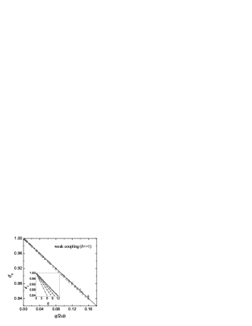
Figure 3: $d_{q}$ as a function of the rescaled variable $q/2\pi b$ in the weak-coupling regime ($b\gg 1$) for several $b$ values: $6$ (squares), $8$ (triangles), $10$ (diamonds), and $12$ (circles); the solid line represents the nonlinear $\sigma$-model estimate, Eq. (3). The inset shows the same data on the scale $q$; solid lines are fits to the form $d_{q}=1-c_{b}q$.

III.2 Strong-coupling regime ($b\ll 1$)

We have also calculated $d_{q}$ for the critical wave functions of Hamiltonian (2) in the strong-coupling regime for which, as we already mentioned, there are no analytical predictions for values of $q\lesssim b\ll 1$. The only analytical estimate in this regime was obtained for $q>1/2$, based on a resonance pairs approximation, in Ref. 22. $\tau_{q}\simeq 4b\Gamma(q-\tfrac{1}{2})/\sqrt{\pi}\Gamma(q-1)$ found diverges at $q=1/2$ and for smaller values of $q$ this approximation completely breaks down.

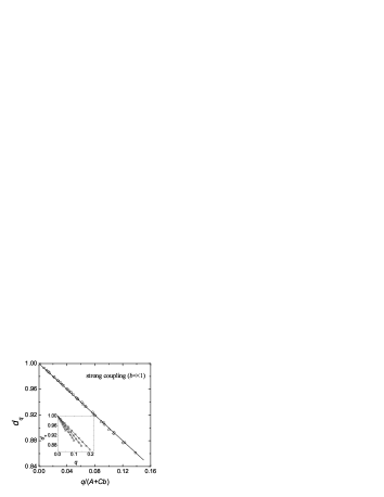
Figure 4: As in Fig. 3, for the strong-coupling regime ($b\ll 1$): $b=0.05$ (squares), $0.1$ (triangles), $0.15$ (diamonds), and $0.2$ (circles). The solid line corresponds to Eq. (8). The straight lines in the inset are fits to the form $d_{q}=1-c_{b}q$.

Figure 4 shows the same extrapolated values of $d_{q}$ as in Fig. 3 in the strong-coupling regime ($b\ll 1$). The values of $b$ reported are $0.05$ (squares), $0.1$ (triangles), $0.15$ (diamonds), and $0.2$ (circles), and the corresponding slopes $c_{b}$ are summarized in Fig. 5 (solid circles). As in the weak disorder case, a linear dependence of $d_{q}$ on $q$ is found for $q\lesssim b$. In order to collapse all data points onto a single straight line, as was done for the opposite limit $b\gg 1$, we propose the relation $1/c_{b}=A+Cb$ for the slopes, where $A\neq 0$ and $C$ are two fitting parameters (see inset of Fig. 5). The collapse of the data is evident from the main panel of Fig. 4, when these data are represented as a function of the rescaled variable $q/(A+Cb)$. Hence, the $q$ dependence of $d_{q}$ in the limit $b\ll 1$ can be described by the linear relation

$$d_{q}=1-\frac{q}{A+C\,b}\;,\quad q\lesssim b\;.$$ (8)

This equation constitutes the main result of the present paper. Thus, our results suggest the intriguing possibility that the linear dependence of $d_{q}$ on $q$ seems to be a generic law valid in all regimes. Although this is a conjecture at the present state, we expect that it will stimulate further analytical work.

Figure 5: The inverse slope $1/c_{b}$ (solid circles) of the fractal dimension as a function of the parameter $b$ of the PRBM model. The solid lines represent the analytical asymptotic ($b\gg 1$) result $2\pi b$ and the strong-coupling ($b\ll 1$) result proposed in this work, $A+Cb$. The small-$b$ behavior of $1/c_{b}$ is reported in the inset; the straight line is a linear fit to the form $A+Cb$.

The inverse slope $1/c_{b}$ of $d_{q}$ is depicted on a log-log plot in Fig. 5 (solid circles) as a function of parameter $b$ of the PRBM model. The inset shows the small-$b$ dependence of $1/c_{b}$, from which the linear behavior on $b$ is evident; the straight line is a linear fit to the proposed form with parameters $A=0.580\pm 0.009$ and $C=4.17\pm 0.08$. The numerical calculations agree perfectly with the analytical asymptotic in the weak-coupling regime $b\gg 1$, $1/c_{b}=2\pi b$, and with the form proposed in this work for the strong-coupling regime $b\ll 1$, $1/c_{b}=0.58+4.17b$.

IV Summary

In this paper we have calculated the fractal dimensions $d_{q}$ of the wave functions for 1D disordered systems with long-range transfer terms at criticality. The leading finite-size corrections to $d_{q}$ decay algebraically with exponents equal to $-1$. At the infinite-size limit, we have confirmed that, according to theoretical predictions, $d_{q}$ is linearly dependent on $q$ in the weak-coupling regime. Our calculations strongly suggest that this behavior is also valid at strong coupling. So, the linear dependence of $d_{q}$ on $q$ seems to be a generic law valid in all disorder regimes.

The question arises as to whether these results are applicable to other quantum systems, particularly in the 3D Anderson transition that occurs in the strong disorder domain, and whose similarity with the PRBM model at $b=0.3$ has been demonstrated for several critical magnitudes.CO02

- (1) H.G.E. Hentschel and I. Procaccia, Physica D 8, 435 (1983).
- (2) M. Janssen, Int. J. Mod. Phys. B 8, 943 (1994); B. Huckestein, Rev. Mod. Phys. 67, 357 (1995).
- (3) V.I. Falko and K.B. Efetov, Europhys. Lett. 32, 627 (1995); Phys. Rev. B 52, 17413 (1995).
- (4) A.D. Mirlin, Phys. Rep. 326, 259 (2000); F. Evers and A.D. Mirlin, Phys. Rev. Lett. 84, 3690 (2000).
- (5) E. Cuevas, M. Ortuño, V. Gasparian, and A. Pérez-Garrido, Phys. Rev. Lett. 88, 016401 (2002).
- (6) K.B. Efetov, Adv. Phys. 32, 53 (1983).
- (7) F. Wegner, Z. Phys. B 36, 209 (1980); C. Castellani and L. Peliti, J. Phys. A 19, L429 (1986); B.L. Altshuler, V.E. Kravtsov, and I.V. Lerner, Zh. Eksp. Teor. Fiz. 91, 2276 (1986) [Sov. Phys. JETP 64, 1352 (1986)].
- (8) A.D. Mirlin, Y.V. Fyodorov, F.M. Dittes, J. Quezada, and T.H. Seligman, Phys. Rev. E 54, 3221 (1996).
- (9) Andreas W. W. Ludwig, Matthew P. A. Fisher, R. Shankar, and G. Grinstein, Phys. Rev. B 50, 7526 (1994).
- (10) C.C. Chamon, C. Mudry, and X.-G. Wen, Phys. Rev. Lett. 77, 4194 (1996); H.E. Castillo, C.C. Chamon, E. Fradkin, P.M. Goldbart, and C. Mudry, Phys. Rev. B 56, 10668 (1997).
- (11) David Carpentier and Pierre Le Doussal, Phys. Rev. E 63, 026110 (2001).
- (12) M.J. Bhaseen, I.I. Kogan, O.A. Soloviev, N. Taniguchi, and A.M. Tsvelik, Nucl. Phys. B 580, 688 (2000).
- (13) D.A. Parshin and H.R. Schober, Phys. Rev. B 57, 10232 (1998).
- (14) H. Potempa and L. Schweitzer, Phys. Rev. B 65, 201105(R) (2002).
- (15) P.W. Anderson, Phys. Rev. 109, 1492 (1958).
- (16) L.S. Levitov, Europhys. Lett. 9, 83 (1989); Phys. Rev. Lett. 64, 547 (1990).
- (17) L.S. Levitov, Ann. Phys. (Leipzig) 8, 697 (1999).
- (18) Clare C. Yu, Phys. Rev. Lett. 63, 1160 (1989).
- (19) R.N. Bhatt and P.A. Lee, Phys. Rev. Lett. 48, 344 (1982).
- (20) P. Cizeau and J.P. Bouchaud, J. Phys. A 26, L187 (1993).
- (21) A.V. Balatsky and M.I. Salkola, Phys. Rev. Lett. 76, 2386 (1996).
- (22) A.D. Mirlin and F. Evers, Phys. Rev. B 62, 7920 (2000).
- (23) E. Cuevas, V. Gasparian, and M. Ortuño, Phys. Rev. Lett. 87, 056601 (2001); E. Cuevas, Phys. Rev. B 66, 233103 (2002).
- (24) I. Varga and D. Braun, Phys. Rev. B 61, R11859 (2000); Imre Varga, ibid. 66, 094201 (2002).
- (25) E. Cuevas, Phys. Rev. B 68, 024206 (2003).
- (26) V.E. Kravtsov and K.A. Muttalib, Phys. Rev. Lett. 79, 1913 (1997).
- (27) V.E. Kravtsov and A.M. Tsvelik, Phys. Rev. B 62, 9888 (2000).
- (28) E. Cuevas, Phys. Rev. Lett. 83, 140 (1999); E. Cuevas, E. Louis, and J.A. Vergés, ibid. 77, 1970 (1996).
- (29) Ashvin Chhabra and Roderick V. Jensen, Phys. Rev. Lett. 62, 1327 (1989).
- (30) Th. Jonckheere and J.M. Luck, J. Phys. A 31, 3687 (1998).