Solitonic transmission of Bose-Einstein matter waves

Abstract

We consider a continuous atom laser propagating through a wave guide with a constriction. Two different types of transmitted stationary flow are possible. The first one coincides, at low incident current, with the non-interacting flow. As the incident flux increases, the repulsive interactions decrease the corresponding transmission coefficient. The second type of flow only occurs for sufficiently large incident currents and has a solitonic structure. Remarkably, for any chemical potential there always exists a value of the incident flux at which the solitonic flow is perfectly transmitted.

The transport properties of matter confined to small structures display distinct quantum effects qualitatively different from those observed at macroscopic scales. These are grounded on global phase coherence throughout the sample and can be, in many cases, understood within single particle pictures, without referring to any specific details of the system. As a result, they arise in many different fields (electronic systems, atomic physics, electromagnetism, acoustics) [2, 3, 4]. Some examples are (weak and strong) localization, Bloch oscillations and conductance quantization.

Recent experimental developments in the physics of Bose-Einstein condensation (BEC) of dilute vapor (in particular the microchip guiding technique) open up the prospect of studying coherent transport phenomena using guided atom lasers [5]. Besides, because of the extraordinary control over these systems, they offer a unique opportunity to go beyond the single particle behavior, and to study specific effects induced by interaction. In the present article we focus on a simple situation, where a BEC matter wave propagates through a guide with a constriction  [6]. By an adiabatic approximation, the three–dimensional flow is reduced to one dimension, where the atoms now feel, due to the constriction, a longitudinal step–like potential of height $V_{0}$. In the absence of interaction, the transmission $T$ does not depend on the incident current but only on the beam’s energy; $T$ is always lower than unity and tends to this limit when the energy of the beam is large compared to $V_{0}$. In the following we consider atoms with a repulsive effective interaction characterized by a scattering length $a_{sc}>0$. The most salient features of the flow are all at variance with respect to the non-interacting case: (i) the transmission coefficient depends on the current, (ii) at given chemical potential, there exists a maximum transmitted current above which no stationary flow exists, (iii) at a given current, several distinct stationary solutions with different $T$ are possible and (iv) for any chemical potential larger than $V_{0}$, there is a particular value of the incident current which induces total transmission.

Consider a continuous atom laser incident on a constriction of a waveguide. Within the adiabatic approximation [7] the transverse motion is restricted to the lowest transverse eigen-state. The constriction affects the longitudinal motion via an effective step-like potential whose magnitude is fixed by the ground state energy of the transverse Hamiltonian. For a BEC system, the adiabatic approximation implies that the condensate wave function can be cast in the form (see Ref. [8]),

$$\Psi(\vec{r},t)=\psi(x,t)\phi(\vec{r}_{\perp};n;x)\;,$$ (1)

where $\psi(x,t)$ describes the motion along the axis of the laser (the beam is flowing along the positive $x$ direction). $\phi$ is the equilibrium wave function (normalized to unity) in the transverse $(\vec{r}_{\perp})$ direction. It depends parametrically on the longitudinal density $n(x,t)=\int d^{2}r_{\perp}|\Psi|^{2}=|\psi(x,t)|^{2}$. The beam is confined in the transverse direction by a trapping potential $V_{\perp}(\vec{r}_{\perp};x)$, which is $x$-dependent in the region of the constriction. Then, the longitudinal wave equation reads [8, 9] (in units where $\hbar=m=1$)

$$-\frac{1}{2}\partial_{xx}\psi+\Big{\{}V_{\parallel}(x)+\epsilon[n(x,t);x]\Big{\}}\,\psi=i\,\partial_{t}\psi\;.$$ (2)

In (2), $V_{\parallel}(x)$ represents an effective longitudinal potential due to the constriction. If, to be specific, we consider a transverse harmonic confinement with pulsation $\omega_{\perp}(x)$, then $V_{\parallel}(x)=\omega_{\perp}(x)-\omega_{\perp}(-\infty)$ (energy is measured with respect of the ground state energy of the non interacting transverse Hamiltonian far before the constriction). $\epsilon(n;x)$ is a nonlinear term describing the mean field interaction averaged over a transverse slice of the beam. One has $\epsilon(n;x)=2\omega_{\perp}(x)\,na_{sc}$ in the low density regime ($na_{sc}\ll 1$), and $\epsilon(n;x)=2\omega_{\perp}(x)\sqrt{na_{sc}}$ in the high density regime ($na_{sc}\gg 1$) [8, 9].

Our purpose is to determine the transmission of steady state solutions of (2) where $\psi(x,t)=\exp\{-i\mu t\}A(x)\exp\{iS(x)\}$, with $A$ and $S$ real functions. The density is $n=A^{2}$ and the local velocity is $v=dS/dx$. From Eq. (2) one obtains (i) flux conservation: $n(x)v(x)$ is a constant that we denote $J_{\infty}$, and (ii) a Schrödinger-like equation for the amplitude:

$$-\frac{1}{2}\,\frac{d^{2}A}{dx^{2}}+\left\{V_{\parallel}(x)+\epsilon[n(x);x]+\frac{J_{\infty}^{2}}{2\,n^{2}(x)}\right\}A=\mu\,A\,.$$ (3)

To define the scattering problem one needs to study the asymptotic behavior of the flow far from the constriction. Far upstream $V_{\parallel}(x\to-\infty)=0$ and the non-linear term in (2) looses its explicit $x$ dependence, taking the simpler form $\epsilon[n(x,t)]$. Thus, in this region, (3) admits a first integral of the form [9] :

$$\frac{1}{2}\left(\frac{dA}{dx}\right)^{2}+W[n(x)] = E_{cl}\;$$ (4)

$$\mbox{with}\;W(n) = -\varepsilon(n)+\mu\,n+\frac{J_{\infty}^{2}}{2\,n}\;,$$ (5)

where $\varepsilon(n)=\int_{0}^{n}\epsilon(\rho)d\rho$ and $E_{cl}$ is an integration constant. Eq. (4) has a simple interpretation in terms of classical dynamics. It expresses the energy conservation of a fictitious classical particle with “position” $A$ and “time” $x$, moving in a potential $W$; $E_{cl}$ being the total energy of this particle. Eq. (4) is thus integrable by quadrature, and the density profile can be deduced from the plot of Fig. 1. Small values of $E_{cl}-W(n_{1})$ correspond to small density oscillations, whereas the highest acceptable value is $E_{cl}=W(n_{2})$, corresponding to a gray soliton.

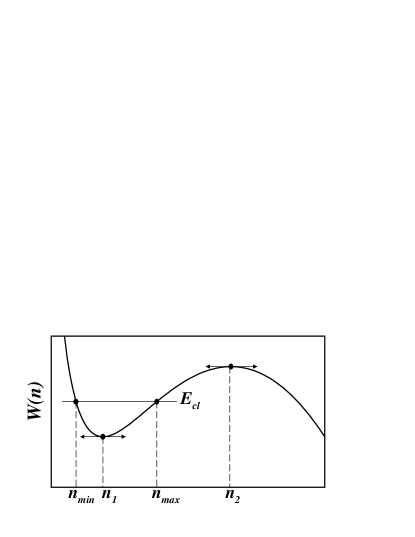
FIG. 1.: $W$ as a function of $n$. $n_{1}$ and $n_{2}$ are the zeros of $dW/dn$. At a given $E_{cl}$, the up-stream density (or equivalently the “position” of the fictitious particle) oscillates between $n_{min}$ and $n_{max}$ defined by $W(n_{min})=W(n_{max})=E_{cl}$.

In the far down-stream region, $V_{\parallel}(x\to+\infty)$ also takes a constant value $V_{0}=\omega_{\perp}(+\infty)-\omega_{\perp}(-\infty)>0$. Hence, (3) admits, in this region, a first integral analogous of (4) where, due to the change in $\omega_{\perp}$, $\epsilon(n)$ (resp. $\varepsilon(n)$) takes a different form which we denote $\epsilon_{0}(n)$ (resp. $\varepsilon_{0}(n)$). The new form of $W(n)$ is denoted $W_{0}(n)$ and the new constant of integration is $E_{cl}^{0}$:

$$\frac{1}{2}\left(\frac{dA}{dx}\right)^{2}+W_{0}[n(x)] = E^{0}_{cl}\;$$ (6)

$$\mbox{with}\;W_{0}(n) = -\varepsilon_{0}(n)+(\mu-V_{0})\,n+\frac{J_{\infty}^{2}}{2\,n}\;.$$ (7)

It follows from general arguments on the dispersion of elementary excitations of Eq. (2) that the physically acceptable boundary conditions of Eq. (3) correspond to a constant far down-stream density (see [9]). The asymptotic $x\to+\infty$ density should thus be equal either to $n_{1,0}$ (we denote this as “case A”), or to $n_{2,0}$ (case B); $n_{1,0}$ and $n_{2,0}$ – being the analogous of $n_{1}$ and $n_{2}$ of Fig. 1 – are extrema of $W_{0}(n)$. They are solutions of

$$\mu=\epsilon_{0}(n)+V_{0}+\frac{J_{\infty}^{2}}{2\,n^{2}}\;.$$ (8)

In the non-interacting case the term $\varepsilon_{0}(n)$ is absent from $W_{0}(n)$ which has only one minimum ($n_{10}$). Case A is therefore the only possible solution in non-interacting systems. Case B describes new non-perturbative effects related to interaction. It corresponds to an asymptotic down-stream density which is part of a gray soliton.

There exists a maximum value $J_{\infty}^{max}$ of $J_{\infty}$ above which Eq. (8) admits no solution: as $J_{\infty}$ is increased (keeping $\mu$ and $V_{0}$ fixed), the two extrema of $W_{0}(n)$ move toward each other, until they coalesce and disappear. This marks the onset of a time–dependent flow. If, to be specific, we consider the case $\epsilon_{0}(n)=g_{0}\,n^{\nu_{0}}$, then

$$J_{\infty}^{max}=\left[\frac{2}{\nu_{0}+2}(\mu-V_{0})\right]^{\frac{1}{\nu_{0}}+\frac{1}{2}}\sqrt{\nu_{0}}\;g_{0}^{-1/\nu_{0}}\;.$$ (9)

The scattering process is now well defined. It corresponds to the matching between two asymptotic densities described by the classical motion of a particle of energy $E_{cl}$ in a potential $W(n)$ at $x\to-\infty$, and of energy $E_{cl}^{0}$ in a potential $W_{0}(n)$ at $x\to+\infty$ (with $E_{cl}^{0}$ either equal to $W_{0}(n_{1,0})$ or to $W_{0}(n_{2,0})$). Eq. (3) being non-linear, an important question is how to properly define a transmission and a reflection coefficient; i.e., is it possible to disentangle an incident and a reflected wave in the upstream flow ? We follow here an approach closely related to usual experimental set-ups, and choose to work with an incident and a reflected beam which can be approximated by plane waves. This corresponds to a regime where Eqs. (3,4) can be linearized in the far upstream region. In this regime, for $x\to-\infty$, we write $n(x)=n_{1}+\delta n(x)$ and expand $nW(n)$ to second order in $\delta n$. Then Eq. (4) leads to

$$\left(\frac{d\,\delta n}{dx}\right)^{2}+\kappa_{1}^{2}\delta n^{2}=8(n_{1}+\delta n)[E_{cl}-W(n_{1})]\;,$$ (10)

where $\kappa_{1}^{2}=4(v_{1}^{2}-c_{1}^{2})$, $v_{1}=J_{\infty}/n_{1}$ being the average velocity of the up-stream beam and $c_{1}=[n_{1}(d\epsilon/dn)_{n_{1}}]^{1/2}$ the sound velocity of a beam with constant density $n_{1}$. The linearization (10) is valid provided $|\delta n(x)/n_{1}|\ll\kappa_{1}^{2}/c_{1}^{2}$. In this regime, if one further imposes $v_{1}\gg c_{1}$, the up-stream density oscillations can be analyzed in term of incident and reflected particles (and not quasi-particles). This allows to unambiguously define the incident, reflected, and transmitted current as $J_{i}=(n_{1}+\delta n_{1}/2)v_{1}$, $J_{r}=\delta n_{1}v_{1}/2$ and $J_{t}=n_{1}v_{1}=J_{\infty}$ (where $\delta n_{1}=4[E_{cl}-W(n_{1})]/\kappa_{1}^{2}$). Hence, once $E_{cl}$ is known, the transmission at given incident current $J_{i}$ is determined through

$$E_{cl}=W(n_{1})+\frac{\kappa_{1}^{2}}{4}\delta n_{1}=W(n_{1})+\frac{\kappa_{1}^{2}}{2v_{1}}J_{i}(1-T)\;.$$ (11)

The linearization procedure explained so far is valid in the case of small upstream interaction (this is the essence of the condition $v_{1}\gg c_{1}$). However, all interaction effects are fully taken into account in the down-stream region, where they are indeed more important (the constriction acts as a barrier which lowers the velocity of the down-stream flow and, by flux conservation, increases its density [10]). In the following we solve the exact non-linear equation (3) and use the linearization procedure only to define the transmission coefficient $T$. Thus, the results presented below are of very general validity, but their analysis in term of transmission coefficient is only correct in so far as the linearization procedure is valid.

The method is now the following: for a given $\mu$ and $J_{i}$, assume a particular value of $T$. This determines $J_{\infty}=T\,J_{i}$, fixes the form of the function $W_{0}(n)$, the value of $n(+\infty)$ (it is equal to $n_{1,0}$ in case A and to $n_{2,0}$ in case B) and of $E_{cl}^{0}=W_{0}[n(+\infty)]$. Integrating (3) backwards from $x=+\infty$ to $x=-\infty$ yields $E_{cl}$, which should be compatible with (11). If not, the value of $T$ has to be modified until self-consistency is achieved.

To understand the physical picture we consider an abrupt step-like constriction. In this geometry, numerical integration of (3) can be bypassed because $E_{cl}$ is simply expressed in terms of $E_{cl}^{0}$ (see Eq. (12)). However, the adiabatic approximation (1) is based on the assumption that the typical longitudinal length scale is much larger than the transverse one. This is clearly violated by an abrupt constriction. Nevertheless, in certain parameter ranges, the adiabatic approximation remains valid. In order to illustrate this point we compute the transmission of non-interacting atoms [11], for which the exact solution can be obtained numerically. We thus consider a linear wave moving in a guide with harmonic confinement whose transverse pulsation changes abruptly (at $x=0$ say) from $\omega_{\perp}^{<}$ (up-stream) to $\omega_{\perp}^{>}=\alpha\,\omega_{\perp}^{<}$ (down-stream), with $\alpha>1$. The incident atoms occupy the transverse ground state of the up-stream potential. The numerical solution of the problem can be worked out by a straightforward 3D generalization of the procedure devised in Ref. [12] for studying a similar 2D problem. We denote the transmission $T^{\scriptscriptstyle L}$, the superscript recalling that we are in a linear (i.e., non-interacting) regime. The result for $T^{\scriptscriptstyle L}$ is presented in Fig. 2 for $\alpha=2$ and $\alpha=3$. The vertical bars indicate the location of the energies of the reflected (thin lines) and transmitted (thick lines) channels. Conservation of angular momentum along the longitudinal axis imposes selection rules between channels. These rules effectively forbid half of the energetically allowed channels, and those henceforth do not play any role in the transmission.

Within the adiabatic approximation, the constriction is described by an abrupt longitudinal step potential of height $V_{0}=\omega_{\perp}^{>}-\omega_{\perp}^{<}$. The corresponding transmission is $T^{\scriptscriptstyle L}_{adia}=4[\mu(\mu-V_{0})]^{1/2}(\sqrt{\mu}+\sqrt{\mu-V_{0}})^{-2}$ (represented by a dashed curve in Fig. 2). The onset of transmission occurs at $\mu=V_{0}$, i.e., $\mu/\omega_{\perp}^{<}=\alpha-1$. One notices in the figure that when $\mu$ is increased from this value, the adiabatic approximation is initially quite accurate. However, at larger values of $\mu$ deviations from adiabaticity are clearly visible. For $\alpha=2$, a sudden lowering of $T^{\scriptscriptstyle L}$ occurs when a new reflected channel opens at $\mu/\omega_{\perp}^{<}=2$ (in all the following we denote as “open channels” those allowed by energy conservation and symmetry rules). From there on, $T^{\scriptscriptstyle L}$ diminishes until a new transmission channel opens, at $\mu/\omega_{\perp}^{<}=5$. At this point, a sudden increase of $T^{\scriptscriptstyle L}$ is observed. At large values of $\mu$, $T^{\scriptscriptstyle L}$ tends to unity, as it should. For $\alpha=3$, the process is similar, but the breakdown of the adiabatic approximation occurs earlier because the opening of the initial transmitted channel – at $\mu/\omega_{\perp}^{<}=2$ – coincides with that of the first allowed excited reflected channel.

In the following we will concentrate on the region $\mu/\omega_{\perp}^{<}\hbox{\lower 3.44444pt\hbox{$\,\buildrel>\over{\sim}\,$}}\alpha-1$ where the adiabatic approximation is well justified and where, as we shall now see, non-linear effects may induce strong modifications of the transmission.

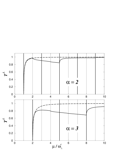
FIG. 2.: Solid curve: transmission $T^{\scriptscriptstyle L}$ of a linear wave as a function of $\mu$ for $\alpha=2$ (top) and $\alpha=3$ (bottom). Dashed curve: adiabatic approximation. In each plot the vertical thick (thin) lines indicate the location of the transverse eigen-energies in the down-stream (up-stream) confining potential.

We now turn to the non-linear problem and consider the case $V_{\parallel}(x<0)=0$, $\epsilon(n;x<0)=\epsilon(n)$ and $V_{\parallel}(x>0)=V_{0}$, $\epsilon(n;x>0)=\epsilon_{0}(n)$. Eq. (3) admits the first integral (4) for all $x\leq 0$ and (6) for all $x\geq 0$. $E_{cl}$ is determined through $E_{cl}^{0}$ by imposing continuity of $A$ and $A^{\prime}$ at $x=0$:

$$E_{cl}-W[n(0)]=E_{cl}^{0}-W_{0}[n(0)]\;.$$ (12)

Let’s consider case A first. The asymptotic down-stream density is $n_{1,0}$ and thus one has, for all $x\geq 0$, $n(x)=n_{1,0}$ (the fictitious classical particle remains at the bottom of the potential well $W_{0}$). In particular, $n(0)=n_{1,0}$ and the matching (12) determines $E_{cl}$ uniquely. The value of $T$ is denoted $T^{\scriptscriptstyle A}$ in this case.

Case B is more interesting because the structure of the down-stream solution is richer: $n(x\geq 0)$ being part of the profile of a gray soliton, $n(0)$ can be varied continuously provided the matching (12) is fulfilled at a value acceptable for Eq. (4). Effectively, the only restriction imposed is that $n_{min}<n(0)<n_{max}$ ($n_{min}$ and $n_{max}$ are defined in Fig. 1). As a result, for fixed $\mu$ and $J_{i}$, $E_{cl}$ is not uniquely determined by $n(+\infty)$, and the transmission $T^{\scriptscriptstyle B}$ varies between 0 and a value that we denote as $T^{\scriptscriptstyle B}_{max}$.

To be specific, we consider a continuous beam of ²³Na atoms propagating through a guide with a transverse confinement $\omega_{\perp}^{<}=2\pi\times 2$ kHz (in the region $x<0$), to which we impose a narrowing $\omega_{\perp}^{>}=2\pi\times 6$ kHz (in the region $x>0$). This represents a barrier of height $V_{0}=192$ nK. In the non-interacting case the transmission $T^{\scriptscriptstyle L}$ as a function of $\mu$ is plotted in the bottom part of Fig. 2 ($\alpha=3$). We take $\mu=210$ nK (this corresponds to the kinetic energy of atoms having a velocity of 1.2 cm/s). This value of $\mu$ corresponds, in the non-interacting case, to a regime where the adiabatic approximation holds and yields a transmission $T^{\scriptscriptstyle L}\simeq T^{\scriptscriptstyle L}_{adia}\simeq 0.70$. The repulsive interaction between atoms introduces in Eq. (3) a non-linear term which, in the region $x<0$, reads $\epsilon(n)=gn$ with $g=2\,a_{sc}\,\omega_{\perp}^{<}\,\simeq 530$ nK.nm. In the region $x>0$, the transverse frequency of the guide is multiplied by 3, and thus $\epsilon_{0}(n)=g_{0}n$ with $g_{0}=3\times g$. An important parameter of the system is the maximum transmitted current $J_{\infty}^{max}$ above which no stationary flow can exist in the down-stream part of the guide. From Eq. (9) (with $\nu_{0}=1$) one obtains $J_{\infty}^{max}\simeq 1.6\times 10^{4}$ atom/s.

Fig. 3 summarizes the results obtained. The linearization condition $v_{1}\gg c_{1}$ is extremely well satisfied in the whole range of incident currents considered (the less favorable case occurs at large $J_{i}$, where $v_{1}\simeq 25\,c_{1}$). The horizontal dashed line is the value of the transmission coefficient of non-interacting atoms : $T^{\scriptscriptstyle L}\simeq 0.7$. It is current independent. When the current is increased from zero, $T^{\scriptscriptstyle A}$ decreases from this value down to $T^{\scriptscriptstyle A}\simeq 0.5$. At this point (located with a black spot on the figure), $J_{\infty}(=T^{\scriptscriptstyle A}J_{i})$ is equal to $J_{\infty}^{max}$, and a stationary flow of type A is no longer permitted (actually it bifurcates to a type B solution). The prominent feature of the behavior of $T^{\scriptscriptstyle A}$ as a function of $J_{i}$ is its decrease compared to the non-interacting value $T^{\scriptscriptstyle L}$. The physical reason behind this phenomenon is simple: the available kinetic energy necessary to step over the barrier is reduced when the interaction energy increases, i.e., when the incident current increases. This picture is supported by a perturbative treatment which accurately describes the flow at low incident current ($J_{i}\ll J_{\infty}^{max}$) and confirms that the decrease of $T^{\scriptscriptstyle A}$ corresponds to an increased fraction of the interaction energy in the chemical potential.

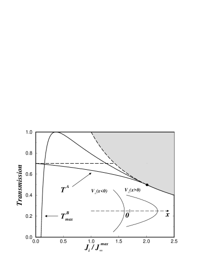
FIG. 3.: $T^{\scriptscriptstyle A}$ and $T^{\scriptscriptstyle B}_{max}$ as a function of $J_{i}/J_{\infty}^{max}$ (at fixed $\mu=210$ nK). The horizontal dashed line is the transmission $T^{\scriptscriptstyle L}$ of non-interacting atoms. The gray zone above the dashed hyperbola (of equation $T=J_{\infty}^{max}/J_{i}$) is a region where no stationary flow exists. Inset: Schematic of the constriction’s geometry.

Case B being mediated via interaction, does not exist for low current. It exists only above a critical current $(2g_{0})^{-1}(\mu-V_{0})^{2}(8\mu)^{-1/2}\simeq 1.5\times 10^{3}$ atom/s $\simeq 0.1\,J_{\infty}^{max}$. From this point, $T^{\scriptscriptstyle B}_{max}$ increases rapidly up to 1 (reached at $J_{i}\simeq 0.45\,J_{\infty}^{max}$ in the case of Fig. 3), and then decreases down to a point where one can show that it exactly meets the end point of $T^{\scriptscriptstyle A}$. From there on, the value of $T^{\scriptscriptstyle B}$ is limited by the condition that the flow should be stationary, and one has $T^{\scriptscriptstyle B}_{max}=J_{\infty}^{max}/J_{i}$, which coincides with the dashed hyperbola in Fig. 3. We emphasize that stationary solutions of type $B$ with arbitrary transmission $0\leq T^{\scriptscriptstyle B}\leq T^{\scriptscriptstyle B}_{max}$ exists for any current above the critical one.

The nonlinear transport induced by the repulsive two-body interaction has therefore a non-trivial consequence: new solutions – of solitonic character – emerge; they allow for an increased transmission. This contrasts with the behavior of case A where the transmission is lowered by the interaction. One can show that, for any value of $\mu>V_{0}$, there always exists a value of $J_{i}$ such that complete transmission exists in case B. The profile for $T^{\scriptscriptstyle B}_{max}=1$ consists of a constant up-stream density $n(x\leq 0)=n_{1}$ connected at $x=0$ to half a soliton. Fig. 4 displays the density profiles of two stationary flows (case $A$ and case $B$ at $T^{\scriptscriptstyle B}=T^{\scriptscriptstyle B}_{max}=1$) at an incident current $J_{i}=0.36\,J_{\infty}^{max}$ (see Fig. 3). Note the significant difference in the densities of the up-stream and down-stream profiles, a purely nonlinear effect mediated by a solitonic profile. We have performed numerical computations that show that the same type of solution also exists for smooth constrictions and that they are dynamically stable, as confirmed by a Bogoliubov analysis. The interactions can thus have two different and, in some sense, opposite consequences on the transport properties of a condensate flow. They diminish the transmission in some instances (case A), but also allow for new stationary flows that can be perfectly transmitted (case B) [13].

FIG. 4.: Density profiles (in dimensionless units) for the constriction defined in the text, at incident current $J_{i}=0.36\,J_{\infty}^{max}$ (flowing from left to right) and chemical potential $\mu=210$ nK. Thick solid line: solitonic flow with $T^{\scriptscriptstyle B}=T^{\scriptscriptstyle B}_{max}=1$; thin solid line: type-A flow with $T^{\scriptscriptstyle A}=0.7$.

We have restricted our analysis to stationary configurations, but dynamical effects are certainly of interest. Amongst these, one could address the question of the transient that exists before stationarity is reached, or the nature of the flow in parameter regions where stationarity is not possible. An other open problem, that clearly deserves investigation, is the dynamical selection of the different types of stationary profiles discussed above: given an initial low density flow (which, from Fig. 3, is of type A), which branch (A or B) will be followed when the incident flux increases ?

There are different ways to experimentally realize the effect discussed in the present work, namely enhanced solitonic transmission of matter waves. We have studied one possible implementation, where the step–like potential in the longitudinal motion of the condensate is produced by a constriction of the guide. An other possibility is to apply a blue-detuned laser beam on the region $x>0$ of a condensate propagating along a guide of constant diameter. In this case, the characteristics of the flow and the barrier should be easily controlled by modifying the laser’s frequency, intensity and waist, thus allowing for a neater experimental observation of the above predicted transport phenomena [14].

We acknowledge stimulating discussions with D. Guéry-Odelin. L.P.T.M.S. is Unité Mixte de Recherche de l’Université Paris XI et du CNRS, UMR 8626.

REFERENCES

- [1] Present address: Max Planck Institut für Physik komplexer Systeme, Nöthnitzer Str. 38, 01187 Dresden, Germany.
- [2] P. Sheng, Introduction to Wave Scattering, Localization, and Mesoscopic Phenomena (Academic Press, 1995).
- [3] Y. Imry, Introduction to Mesoscopic Physics (Oxford University Press, New York, 1997).
- [4] M. Raizen, C Salomon and Q. Niu, Physics Today 50(7), 30 (1997).
- [5] W. Hänsel et al., Nature 413, 498 (2001); K. Bongs et al., Phys. Rev. A 63, 031602(R) (2001); J. Fortágh et al., Appl. Phys. Lett. 81, 1146 (2002); A. E. Leanhardt et al., Phys. Rev. Lett. 89, 040401 (2002); P. Cren et al., Eur. Phys. J. D 20, 107 (2002).
- [6] An analogous configuration for cold, non-condensed and non-interacting, atoms has been studied by J. H. Thywissen, R. M. Westervelt, and M. Prentiss, Phys. Rev. Lett. 83, 3762 (1999). Related aspects of the propagation of cold atoms are discussed by T. Lahaye, P. Cren, C. Roos, D. Guéry-Odelin, Comm. Nonlin. Sci. Num. Sim. 8, 315 (2003).
- [7] L. I. Glazman, G. B. Lesovik, D. E. Khmel’nitskii and R. I. Shekhter, Pisma Zh. Eksp. Teor. Fiz. 48, 218 (1988) [JETP Lett. 48, 238 (1988)].
- [8] A. D. Jackson, G. M. Kavoulakis, and C. J. Pethick, Phys. Rev. A 58, 2417 (1998).
- [9] P. Leboeuf and N. Pavloff, Phys. Rev. A 64, 033602 (2001).
- [10] Down-stream interaction effects are further amplified by the effective nonlinear term which increases with transverse confinement.
- [11] The wide range of validity of the adiabatic approximation is well established for linear waves (see, e.g., F. Kassubek, C. A. Stafford, and H. Grabert, Phys. Rev. B 59, 7560 (1999)), but much less is known in the nonlinear case (see, J. Liu, B. Wu, and, Q. Niu, Phys. Rev. Lett. 90, 170404 (2003)).
- [12] A. Szafer and A. D. Stone, Phys. Rev. Lett. 62, 300 (1989).
- [13] Other anomalous transport effects have been reported recently, see Yu. Kagan, D. L. Kovrizhin, and L. A. Maksimov, Phys. Rev. Lett. 90, 130402 (2003).
- [14] Besides, the adiabatic approximation is better justified if the potential step for the linear motion results from an external source (in the absence of interaction it is rigorously exact since the problem is separable).