Tunnel magnetoresistance in double spin filter junctions

Abstract

We consider a new type of magnetic tunnel junction, which consists of two ferromagnetic tunnel barriers acting as spin filters (SFs), separated by a nonmagnetic metal (NM) layer. Using the transfer matrix method and the free-electron approximation, the dependence of the tunnel magnetoresistance (TMR) on the thickness of the central NM layer, bias voltage and temperature in the double SF junction are studied theoretically. It is shown that the TMR and electron-spin polarization in this structure can reach very large values under suitable conditions. The highest value of the TMR can reach 99%. By an appropriate choice of the thickness of the central NM layer, the degree of spin polarization in this structure will be higher than that of the single SF junctions. These results may be useful in designing future spin-polarized tunnelling devices.

I Introduction

In the past few years, tunnel magnetoresistance (TMR) in magnetic tunnel junctions consisting of two ferromagnetic metal (FM) electrodes separated by a thin insulator (FM/I/FM) has attracted much attention due to its promising applications in magnetic field sensors and magnetic random access memory [1, 2]. The TMR in FM/I/FM junctions depends on the degrees of electron spin polarization of the two FM electrodes [3], but the lack of nearly perfectly spin-polarized current, and temperature dependence of the polarization, have limited the TMR in these junctions [4, 5]. If we use half-metallic electrodes in the magnetic tunnel junctions, which are completely spin-polarized at $T$=0 K due to complications such as disorder and surface effects, half-metallicity is destroyed and thus the spin polarization and the TMR are decreased [6]. However, by exploiting the spin filtering phenomenon, one can create 100% spin polarization and obtain a giant TMR.

The spin filtering effect in a ferromagnetic semiconductor (FMS) has been demonstrated dramatically in spin-polarized tunnelling experiments [7]. In these experiments, using an Al/EuS/Al tunnel junction, Moodera et al obtained 85% spin polarization for tunnel electrons. In another study with EuSe barrier junctions [8] and in the presence of an external magnetic field, they reported near 100% spin polarization. More recently, LeClair et al [9] from the combination of a spin filter (SF) barrier and a FM electrode, obtained a large TMR in an Al/EuS/Gd tunnel junction, which is a new method for spin injection into semiconductors [10]. When a FMS layer such as EuS is used as a tunnel barrier, due to the spin splitting of the conduction band in the FMS, tunnelling electrons see a spin-dependent barrier height. Thus the probability of tunnelling for one spin channel will be much larger than the other, and a highly spin-polarized current may result. Although the TMR using other SF barriers has also been studied [11, 12, 13], the results have shown only little success.

The TMR in single and double SF junctions has also been investigated theoretically in recent years. Based on the two band model and free-electron approximation [14], Li et al [15] studied the tunnelling conductance and magnetoresistance of FM/FMS/FM junctions. The results showed that a decrease or increase in tunnelling current strongly depends on the magnetization orientations both in the electrodes and in the FMS layer. In another theory with double SF junctions, Worledge et al [16] studied the TMR of the NM (nonmagnetic metal)/FMS/FMS/NM junctions, using a simple model, and obtained a large magnetoresistance. In a recent paper, Wilczynski et al [17] investigated tunnelling in NM/FMS/NM/FMS/NM junctions in a sequential tunnelling regime. They found a strong enhancement of the TMR with increasing spin splitting of the barrier height in the ferromagnetic barriers. However, they have not investigated the effect of electric field and temperature on the tunnel currents and spin polarization. Thus, other aspects of this structure, such as the voltage dependence of TMR, remain to be explained.

In the previous paper [18], using the single-site approximation for the NM/FMS/NM/FMS/NM double SF junction, we studied the effect of the thickness of the central layer on the spin polarization of tunnel electrons at $T$=0 K. We showed that the tunnelling spin polarization has an oscillatory behavior with the thickness, which is due to the spin asymmetry of the reflection at the FMS/NM interfaces.

In this paper, using the transfer matrix method and the free-electron approximation, we have extended our previous work [18] to investigate the effect of the thickness of the central layer, temperature and applied bias on the TMR for tunnelling through a double SF junction. The paper is organized as follows. In section 2, the transfer matrix approach of the spin-polarized tunnelling through the double SF junctions is described. In section 3, the numerical results for the TMR and the spin polarization of the tunnel currents are discussed. The conclusions are summarized in section 4.

II Model and formalism

The system we consider here is a NM/FMS/NM/FMS/NM sandwich structure in the presence of an applied bias $V_{a}$, which is depicted in Fig. 1. For simplicity, we assume the FMS layers, which act as SFs, are made of the same material, while the outer NM electrodes, which are semi-infinite, and the central layer are made of the same metal. This structure is grown in the $x$ direction. In this case, in a free-electron approximation for the spin-polarized tunnelling electrons, the longitudinal part of the effective one-electron Hamiltonian can be written as

$$H_{x}=-\frac{\hbar^{2}}{2m_{j}^{*}}\frac{d^{2}}{dx^{2}}+U_{j}(x)+V_{j}^{\sigma}\ ,$$ (1)

where $m^{*}_{j}$ ($j$=1-5) is the electron effective mass in the $j$th layer and

$$U_{j}(x)=\left\{\begin{array}[]{cc}0,&x<0\ ,\\ -eV_{a}x/(L-c)+U_{2},&0<x<b\ ,\\ -eV_{a}b/(L-c),&b<x<b+c\ ,\\ -eV_{a}(x-c)/(L-c)+U_{4},&b+c<x<L\ ,\\ -eV_{a},&x>L\ ,\end{array}\right.$$ (2)

where $U_{2}$ and $U_{4}$ are, respectively, the barrier heights of the left and right FMS layer at above $T_{C}$, $b$ and $d$ are the barrier widths, $c$ is the width of the middle NM layer and $L=b+c+d$. The third term in Eq. (1) which is a spin-dependent potential, denotes the $s-f$ exchange coupling between the spin of tunnelling electrons and the localized $f$ spins in the $j$th FMS layer. Within the mean field approximation, $V_{j}^{\sigma}$ is proportional to the thermal average of the $f$ spins, $\langle S_{z}\rangle$ (a 7/2 Brillouin function), and can be written as $V_{j}^{\sigma}=-I\sigma\langle S_{z}\rangle$. Here, $\sigma=\pm 1$, which corresponds to $\sigma=\uparrow,\downarrow$, respectively and $I$ is the $s-f$ exchange constant in the FMS layers.

The Schrödinger equation for a barrier layer under the influence of an applied bias can be simplified by a coordinate transformation whose solution is a linear combination of the Airy function Ai[$\rho(z)$] and its complement Bi[$\rho(z)$] [19]. Considering all five regions of the NM/FMS/NM/FMS/NM junction shown in Fig. 1, the eigenfunctions of the Hamiltonian (1) with eigenvalue $E_{x}$ have the following forms:

$$\psi_{j,\sigma}(x)=\left\{\begin{array}[]{cc}A_{1\sigma}e^{ik_{1}x}+B_{1\sigma}e^{-ik_{1}x},&x<0\ ,\\ A_{2\sigma}\mbox{Ai}[\rho_{2\sigma}(x)]+B_{2\sigma}\mbox{Bi}[\rho_{2\sigma}(x)],&0<x<b\ ,\\ A_{3\sigma}e^{ik_{3}x}+B_{3\sigma}e^{-ik_{3}x},&b<x<b+c\ ,\\ A_{4\sigma}\mbox{Ai}[\rho_{4\sigma}(x)]+B_{4\sigma}\mbox{Bi}[\rho_{4\sigma}(x)],&b+c<x<L\ ,\\ A_{5\sigma}e^{ik_{5}x}+B_{5\sigma}e^{-ik_{5}x},&x>L\ ,\end{array}\right.$$ (3)

where the coefficients $A_{j\sigma}$ and $B_{j\sigma}$ are constants to be determined from the boundary conditions and

$$k_{1}=\sqrt{2m_{1}^{*}E_{x}}/\hbar\ ,$$ (4)

$$k_{3}=\sqrt{2m_{3}^{*}(E_{x}+eV_{a}b/(L-c))}/\hbar\ ,$$ (5)

$$k_{5}=\sqrt{2m_{5}^{*}(E_{x}+eV_{a})}/\hbar\ ,$$ (6)

$$\rho_{j,\sigma}(x)=\frac{x}{\lambda_{j}}+\beta_{j,\sigma}\ ,\qquad j=2,4\ ,$$ (7)

with

$$\lambda_{j}=\left[-\frac{(L-c)\hbar^{2}}{2m^{*}_{j}eV_{a}}\right]^{1/3}\ ,$$ (8)

$$\beta_{j,\sigma}=\left\{\begin{array}[]{cc}\frac{(L-c)[E_{x}-U_{j}-V_{j}^{\sigma}]}{eV_{a}\lambda_{j}},&j=2\ ,\\ \frac{(L-c)[E_{x}-U_{j}-V_{j}^{\sigma}-eV_{a}c/(L-c)]}{eV_{a}\lambda_{j}},&j=4\ .\end{array}\right.$$ (11)

Although the transverse momentum ${\bf k_{\parallel}}$ does not appear in the above notations, the effects of the summation over ${\bf k_{\parallel}}$ will be considered in our calculations.

A Transmission coefficients

By using the boundary condition such that the wavefunctions and their first derivatives are matched at each interface point $x_{j}$, i.e. $\psi_{j,\sigma}(x_{j})=\psi_{j+1,\sigma}(x_{j})$ and $(m^{*}_{j})^{-1}[d\psi_{j,\sigma}(x_{j})/dx]=(m^{*}_{j+1})^{-1}[d\psi_{j+1,\sigma}(x_{j})/dx]$, we obtain a matrix formula that connects the coefficients $A_{1\sigma}$ and $B_{1\sigma}$ with the coefficients $A_{5\sigma}$ and $B_{5\sigma}$ as follows:

$$\left[\begin{array}[]{c}A_{1\sigma}\\ B_{1\sigma}\end{array}\right]=M_{total}\left[\begin{array}[]{c}A_{5\sigma}\\ B_{5\sigma}\end{array}\right]\ ,$$ (16)

where

$$M_{total} = \frac{k_{5}}{k_{1}}\left[\begin{array}[]{cc}ik_{1}&\frac{1}{\lambda_{2}}\frac{m_{1}^{*}}{m_{2}^{*}}\\ ik_{1}&-\frac{1}{\lambda_{2}}\frac{m_{1}^{*}}{m_{2}^{*}}\end{array}\right]\left[\begin{array}[]{cc}\mbox{Ai}[\rho_{2\sigma}(x=0)]&\mbox{Bi}[\rho_{2\sigma}(x=0)]\\ \mbox{Ai}^{\prime}[\rho_{2\sigma}(x=0)]&\mbox{Bi}^{\prime}[\rho_{2\sigma}(x=0)]\end{array}\right]$$ (38)

$$\times\left[\begin{array}[]{cc}\mbox{Ai}[\rho_{2\sigma}(x=b)]&\mbox{Bi}[\rho_{2\sigma}(x=b)]\\ \frac{1}{\lambda_{2}}\frac{1}{m^{*}_{2}}\mbox{Ai}^{\prime}[\rho_{2\sigma}(x=b)]&\frac{1}{\lambda_{2}}\frac{1}{m^{*}_{2}}\mbox{Bi}^{\prime}[\rho_{2\sigma}(x=b)]\end{array}\right]^{-1}$$

$$\times\left[\begin{array}[]{cc}\mbox{cos}(k_{3}c)&-\frac{m^{*}_{3}}{k_{3}}\mbox{sin}(k_{3}c)\\ \frac{k_{3}}{m^{*}_{3}}\mbox{sin}(k_{3}c)&\mbox{cos}(k_{3}c)\end{array}\right]$$

$$\times\left[\begin{array}[]{cc}\mbox{Ai}[\rho_{4\sigma}(x=b+c)]&\mbox{Bi}[\rho_{4\sigma}(x=b+c)]\\ \frac{1}{\lambda_{4}}\frac{1}{m^{*}_{4}}\mbox{Ai}^{\prime}[\rho_{4\sigma}(x=b+c)]&\frac{1}{\lambda_{4}}\frac{1}{m^{*}_{4}}\mbox{Bi}^{\prime}[\rho_{4\sigma}(x=b+c)]\end{array}\right]$$

$$\times\left[\begin{array}[]{cc}\mbox{Ai}[\rho_{4\sigma}(x=L)]&\mbox{Bi}[\rho_{4\sigma}(x=L)]\\ \mbox{Ai}^{\prime}[\rho_{4\sigma}(x=L)]&\mbox{Bi}^{\prime}[\rho_{4\sigma}(x=L)]\end{array}\right]^{-1}$$

$$\times\left[\begin{array}[]{cc}ik_{5}&\frac{1}{\lambda_{4}}\frac{m_{5}^{*}}{m_{4}^{*}}\\ ik_{5}&-\frac{1}{\lambda_{4}}\frac{m_{5}^{*}}{m_{4}^{*}}\end{array}\right]^{-1}\left[\begin{array}[]{cc}e^{-ik_{5}L}&0\\ 0&e^{ik_{5}L}\end{array}\right]^{-1}\ .$$

Since there is no reflection in region 5, the coefficient $B_{5\sigma}$ in Eq. (3) is zero. In this case the transmission coefficient of the spin $\sigma$ electron which is defined as the ratio of the transmitted flux to the incident flux, for the double SF structure shown in Fig. 1, can be written as

$$T_{\sigma}(E_{x},V_{a})=\frac{k_{5}m_{1}^{*}}{k_{1}m_{5}^{*}}\left|\frac{1}{M^{11}_{total}}\right|^{2}\ ,$$ (39)

where $M^{11}_{total}$ is the left-upper element of the matrix $M_{total}$ which is defined in Eq. (38). Note that the transmission coefficient depends on the longitudinal energy $E_{x}$, the applied bias $V_{a}$ and the spin orientation.

B Spin polarization and TMR

The spin-dependent current density for single or double SF junctions at a given applied bias $V_{a}$ can be calculated within the free-electron model [20]:

$$J_{\sigma}=\frac{em^{*}_{1}k_{B}T}{4\pi^{2}\hbar^{3}}\int_{0}^{\infty}T_{\sigma}(E_{x},V_{a})\ln\left\{\frac{1+\exp[(E_{F}-E_{x})/k_{B}T]}{1+\exp[(E_{F}-E_{x}-eV_{a})/k_{B}T]}\right\}dE_{x}\ ,$$ (40)

where $k_{B}$ is the Boltzmann constant, $T$ is the temperature, and $E_{F}$ is the Fermi energy.

The degree of spin polarization for the tunnel current is defined by

$$P=\frac{J_{\uparrow}-J_{\downarrow}}{J_{\uparrow}+J_{\downarrow}}\ ,$$ (41)

where $J_{\uparrow}$ $(J_{\downarrow})$ is the spin-up (spin-down) current density. For the double SF junction, this quantity can be obtained when the magnetizations of two FMS layers are in parallel alignment.

The tunnel conductance per unit area is given by $G=\sum_{\sigma}J_{\sigma}/V_{a}$. In this case, the TMR can be described quantitatively by the relative conductance change as

$$\mbox{TMR}=\frac{G_{\uparrow\uparrow}-G_{\uparrow\downarrow}}{G_{\uparrow\uparrow}},$$ (42)

where $G_{\uparrow\uparrow}$ and $G_{\uparrow\downarrow}$ correspond to the conductances in the parallel and antiparallel alignments of the magnetizations in the FMS layers, respectively.

III Numerical results and discussion

The numerical calculations have been performed for a NM/EuS/NM/EuS/NM double SF junction in which, for simplicity, we assume that the EuS layers have the same thickness $b=d$=0.5 nm. The appropriate parameters for EuS which have been used in this paper are: $T_{C}$=16.5 K [21], $S$=7/2, $I$=0.1 eV [22], $m^{*}_{\rm EuS}=1.5$ m_e [23] and $U_{2}=U_{4}=E_{F}$+0.75 eV. In the NM layers, the electron effective mass and the Fermi energy are taken as $m^{*}_{\rm NM}=m_{e}$ and $E_{F}$=1.25 eV. Here $m_{e}$ is referred to the free-electron mass. In this study, we calculate the spin currents, tunnelling spin polarization and the TMR by using Eqs. (40)-(42), respectively. In our considered system, the magnetization orientation (i.e. the $f$ spins’ direction) in the left EuS layer stays fixed but the other EuS layer is free and may be switched back and forth by an external magnetic field (see Fig. 1). Thus, when the magnetizations of two FMS layers are parallel, spin-up and spin-down electrons see a symmetric structure, while for the antiparallel alignment these electrons see an asymmetric structure. This structural asymmetry results from the difference in the two barrier heights for each spin channel.

Figure 2 shows the TMR as a function of the thickness of the central NM layer at $T$=0, 0.45 and 0.9 $T_{C}$, when the bias voltage $V_{a}$=50 mV is applied to the junction. It is obvious that the TMR oscillates with increasing thickness $c$ and have well-defined peaks in which the TMR can reach 99% in some structures. The height of these peaks decreases with increasing $c$. The oscillatory behavior is related to the quantum-well states of the central NM layer and the spin-polarized resonant tunnelling. On the other hand, due to the temperature dependence of spin splitting in the EuS layers, the barrier heights become spin-dependent, so that with decreasing temperature, this spin splitting, and thus the TMR, increases.

To understand the physical origin of the TMR and the oscillations, we study the energy dependence of the transmission coefficients through the double SF junction. In Fig. 3, we have plotted the spin-dependent transmission coefficients at $T$=0 K for $c$=0.50 nm, which corresponds to a flat area between the peaks, and for $c$=0.72 nm, which corresponds to a local maximum in the TMR. Because of the quasibound states in the central NM layer, the transmission coefficients reach unity at the resonance peaks which become sharper in the low incident energy region, since in this energy region the resonance levels are more strongly quantized. The results for $c$=0.50 nm show that there is one resonance level in the quantum well for both spin orientations and magnetic alignments. All these resonance levels are far from the Fermi energy. However, the transmission coefficient for spin-up electrons in the parallel alignment is higher than the antiparallel alignment, and for spin-down electrons in both alignments. Thus, there is a small difference in the current density $J$ (=$J_{\uparrow}+J_{\downarrow}$) in both magnetic configurations, which gives rise to relatively small TMR at this thickness of the central layer. For $c$=0.72 nm the resonance states shift to the lower energy side and a new resonance level slightly below $E_{F}$ appears, which is active only for spin-up electrons in the parallel alignment. Therefore, there is a large difference in the current density $J$ in both alignments and consequently gives rise to large TMR. It is clear from the Fig. 3(b) and 3(d) that, for each thickness $c$, the resonance levels for spin-up and spin-down electrons in the antiparallel alignment coincide. The reason is that, for the antiparallel alignment, electrons with up (down) spin are easy (difficult) to tunnel into the central NM layer, and difficult (easy) to tunnel out of it; thus, both the spin-up and spin-down electrons see the same effective height of the barriers during the tunnelling process through the whole system.

In Fig. 4 we show the TMR as a function of the applied bias at $T$=0 K for the thicknesses $c$ correspond to Fig. 3. With increasing bias voltage, the TMR for $c$=0.50 nm decreases very slowly because, in this range of the applied voltage, the discrepancy between the conductance for the parallel alignment and that for the antiparallel alignment increases only slightly. On the other hand, the results show that, for $c$=0.72 nm at the beginning, the TMR slowly decreases with increasing the bias voltage. However, for the voltages higher than $V_{a}$=80 mV, it quickly decreases. The reason is that, at higher voltages, one of the resonance levels becomes active for both magnetic alignments which drastically reduces the TMR.

It should be noted that, for very low values of the applied bias and the incident energy, a numerical instability is occurred in some of our calculations, which is due to the use of exact Airy functions. This instability is overcome by using the asymptotic forms of Airy functions [19] and numerical analytical methods.

In Fig. 5 we have shown the spin polarization of the tunnelling current versus normalized temperature $T/T_{C}$ for single and double SF junctions to reveal the SF effects of the FMS layers from another point of view. At high temperatures $T>T_{C}$, there is no spin splitting $E_{ex}$ in the conduction band of the EuS layers and the transmission coefficients for two spin channels coincide. Thus there is no TMR and spin polarization effect. As the temperature decreases from $T_{C}$, the barrier heights for spin-up electrons are lowered, while they are raised for spin-down electrons. This temperature dependence of the barrier height, which is attributed to the exchange splitting of the EuS conduction band, greatly increases the tunnelling probability for one spin channel and reduces it for the other. In the parallel alignment, the tunnel current for spin-up electrons is much higher than the spin-down ones, which gives rise to the TMR and spin polarization effect. On further decreasing the temperature, this spin splitting and hence the difference in the barrier heights increases. Therefore, the TMR and spin polarization reach the highest values at $T$=0 K. The highest value of the spin polarization for the single SF junction can reach 77%, which is qualitatively in agreement with the experimental measurements [7] and the theoretical results [24, 25], while for the double SF junction (in the parallel alignment), it approaches 66% for $c$=0.50 nm and 99% for $c$=0.72 nm [18], which is due to the change in the positions of the spin-polarized quasibound states in the quantum well. Therefore, one can see that, for the double SF junctions, the TMR and the spin polarization of the tunnelling current can be controlled by the thickness of the central NM layer, the temperature, and the applied bias.

In this study, the numerical results obtained for the TMR and the degree of spin polarization can be compared with the result of Wilczynski et al [17]. As we discussed above, the enhancement of spin splitting $E_{ex}$ in the conduction band of the FMS layers can be obtained, when the temperature decreases. In this case, the TMR and the spin polarization increases, and this behaviour is in agreement with the result obtained by Wilczynski et al in the sequential tunnelling regime.

IV Summary

Based on the free-electron model, we presented a transfer matrix method for spin-polarized tunnelling through the double SF junctions. The effect of the quantum size, applied bias and temperature on the spin filtering and the spin transport process in the FMS/NM double junctions are examined. Numerical results indicate that the TMR oscillates as the thickness of the central NM layer increases. It is further confirmed that, for some thicknesses of the central NM layer, the spin-polarized resonant tunnelling can gives rise to large values for the spin polarization and the TMR, even at high temperatures ($T<T_{C}$). Therefore, in the system presented here, it is able to select an appropriate applied bias, temperature and the thickness to achieve a maximum TMR and spin polarization.

Although the temperature for observing a 99% TMR is very low and the findings of the paper are not directly applicable to spintronics technology, the results may be useful in designing future spin-polarized tunnelling devices [26].

In the present model, we have neglected the generally important complications, such as the interface roughness, electron-electron interaction, magnetic-domain wells, $f$ spin correlation, etc. These effects can play important roles in the spin transport process and reduce the efficiency of spin filtering.

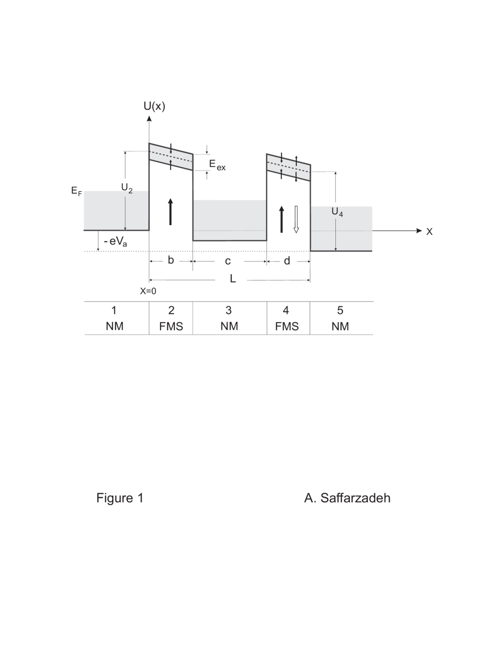
FIG. 1.: Spin-dependent potential profile for NM/FMS/NM/FMS/NM tunnel junctions in the presence of a positive bias $V_{a}$. The broken line in the FMS layers represents the bottom of the conduction band at $T\geq T_{C}$. Below $T_{C}$, due to the exchange splitting $E_{ex}$ in the conduction band, the barrier heights become spin-dependent, as indicated by the thin arrows for spin-up and spin-down electrons. The direction of magnetization in the left FMS layer is fixed in the $+z$ direction, while the magnetization in the right FMS layer is free to be flipped into either the $+z$ or $-z$ direction, as indicated by the filled and hollow arrows, respectively.

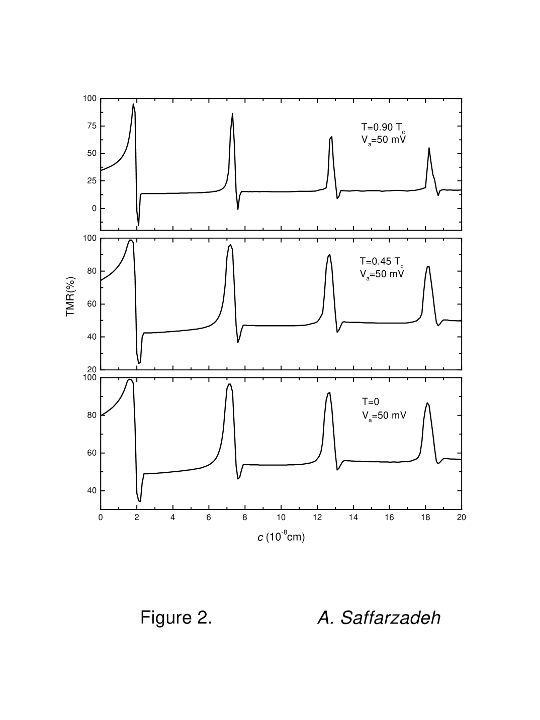
FIG. 2.: TMR as a function of the thickness $c$ in the EuS/NM double SF junction at $T$=0, 0.45 and 0.9 $T_{c}$.

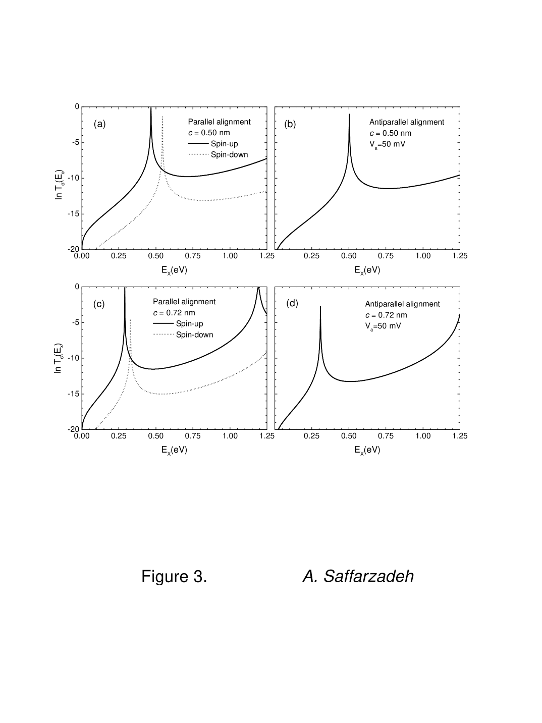
FIG. 3.: Spin-dependent transmission coefficients, $\ln T_{\sigma}(E_{x})$, as a function of energy $E_{x}$ in the EuS/NM double SF junction for $c$=0.50 and 0.72 nm at $T$=0 K.

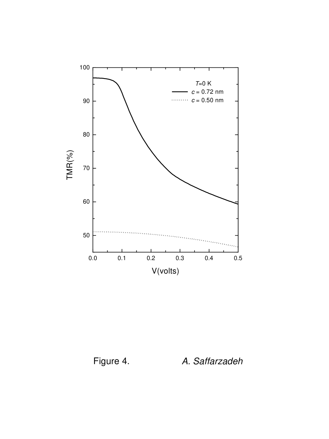
FIG. 4.: TMR as a function of applied bias $V_{a}$ in the EuS/NM double SF junction for $c$=0.50 and 0.72 nm at $T$=0 K.

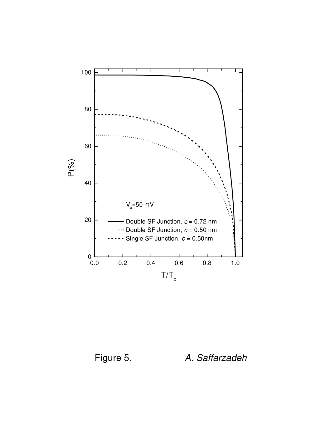
FIG. 5.: Electron-spin polarization $P$ as a function of normalized temperature $T/T_{C}$ for the EuS/NM single and double SF junctions.

REFERENCES

- [1] Moodera J S and Mathon G 1999 J. Magn. Magn. Mater. 200 248
- [2] Inomata K 1999 J. Magn. Soc. Jpn. 23 1826
- [3] Julliere M 1975 Phys. Lett. A 54 225
- [4] Meservey R and Tedrow P M 1994 Phys. Rep. 238 174
- [5] Moodera J S, Kinder L R, Wong T M and Meservey R 1995 Phys. Rev. Lett. 74 3273
- [6] Pickett W E and Moodera J S 2001 Phys. Today 5 39
-
[7]
Moodera J S, Hao X, Gibson G A and Meservey R 1988 Phys. Rev. Lett.
61 637
Hao X, Moodera J S and Meservey R 1990 Phys. Rev. B 42 8235 - [8] Moodera J S, Meservey R and Hao X 1993 Phys. Rev. Lett. 70 853
- [9] LeClair P, Ha J K, Swagten H J M, Kohlhepp J T, van de Vin C H and de Jong W J M 2002 Appl. Phys. Lett. 80 625
- [10] Fiederling R, Keim M, Reuscher G, Ossau W, Schmidt G, Waag A and Molenkamp L 1999 Nature (London) 402 787
- [11] Suezawa Y, Takahashi F and Gondo Y 1992 Jpn. J. Appl. Phys. 31 L1415
- [12] Nowak J and Rauluszkiewicz J 1992 J. Magn. Magn. Mater. 109 79
- [13] LeClair P, Moodera J S and Meservey R 1994 J. Appl. Phys. 76 6546
- [14] Slonczewski J C 1989 Phys. Rev. B 39 6995
- [15] Li Y, Li B Z, Zhang W S and Dai D S 1998 Phys. Rev. B 57 1079
- [16] Worledge D C and Geballe T H 2000 J. Appl. Phys. 88 5277
- [17] Wilczynski M and Barnas J 2001 Sensors and Actuators A 91 188
- [18] Saffarzadeh A 2001 Eur. Phys. J. B 24 149
- [19] Abramowitz M and Stegun I A 1965 Handbook of Mathematical Functions (Dover, New York)
- [20] Duke C B 1969 Tunneling Phenomena in Solids ed. Burstein E and Lundquist S (Plenum, New York)
- [21] Baum G, Kisker E, Mahan A H, Raith W and Reihl B 1977 Appl. Phys. 14 149
- [22] Nolting W, Dubil U and Matlak M 1985 J. Phys. C 18 3687
- [23] Wachter P 1979 Handbook on the Physics and Chemistry of Rare Earths ed. Gschneider K A , Eyring Jr and L (North-Holland, Amsterdam) Ch. 19
- [24] Metzke R and Nolting W 1998 Phys. Rev. B 58 8579
- [25] Saffarzadeh A 2000 Phys. Lett. A 270 353
- [26] Dietl T, Ohno H, Matsukura F, Cibert J and Ferrand D 2000 Science 287 1019