Green’s functions of infinite-$U$ asymmetric Hubbard model: Falicov-Kimball limit

I.V.Stasyuk, O.B.Hera
(Received February 24, 2003)
Abstract

The asymmetric Hubbard model is used in investigating the lattice gas of the moving particles of two types. The model is considered within the dynamical mean-field method. The effective single-site problem is formulated in terms of the auxiliary Fermi-field. To solve the problem an approximate analytical method based on the irreducible Green’s function technique is used. This approach is tested on the Falicov-Kimball limit (when the mobility of ions of either type is infinitesimally small) of the infinite-$U$ case of the model considered. The dependence of chemical potentials on concentration is calculated using the one-particle Green’s functions, and different approximations are compared with the exact results obtained thermodynamically. The densities of states of localized particles are obtained for different temperatures and particle concentrations. The phase transitions are investigated for the case of the Falicov-Kimball limit in different thermodynamic regimes.

Key words: asymmetric Hubbard model, Falicov-Kimball model, dynamical mean-field theory, Green’s functions, phase transitions

PACS: 71.10.Fd, 05.30.Fk, 05.70.Fh

1 Introduction

Strongly correlated electron systems have been a subject of growing interest in recent years. These systems became especially interesting after the discovery of high-$T_{\mathrm{c}}$ superconductivity. In general, the methods used for their description are based on the Hubbard model and its generalizations taking into account strong short-range correlations of particles. Similar models are considered in investigating the ionic conductivity in crystalline materials. Fermi lattice gas models can be mentioned among them. The asymmetric Hubbard model [1] arises by extending the models to the case of the systems with moving ions of two types. The transfer parameters and chemical potentials are different for the ions of different nature. As some special cases, the asymmetric Hubbard model includes the Falicov-Kimball model and the standard Hubbard model. Thereby, it should be mentioned that the asymmetric Hubbard model has been recently obtained as a generalization of the electron Falicov-Kimball model which describes the interactions between itinerant $d$-electrons and localized $f$-electrons by including $f$ $f$ hopping [2]. The model was used in describing the effects related to orbital ordering, as well as to Bose-condensation of electron-hole pairs (which includes a spontaneous ferroelectric polarization) in oxide compounds.

Despite the relative simplicity of these models, the theory of electron spectrum and thermodynamic properties of such systems is far from its final completion. In recent years the essential achievements of the theory of strongly correlated electron systems have been connected with the development of the dynamical mean-field theory (DMFT) [3]. This method is exact in the limit of infinite space dimension ($d=\infty$) and is based on the fact that the irreducible (according to Larkin) part of the one-particle Green’s function is single-sited (at appropriate scaling of transfer parameter).

The central point in this method is the formulation and the solution of the auxiliary single-site problem. In this case a separated lattice site is considered as placed in some effective environment. Since the processes of the particle hopping from the site and returning into the site are taken into account, the mean field acting on the particle states of the site is of a dynamic nature. The field is described by the coherent potential $J_{\sigma}(\omega)$ that should be determined in a self-consistent way from the condition that the same total irreducible (according to Larkin) part defines Green’s functions both in the atomic limit and for the lattice [4, 5, 6]:

$\displaystyle G_{\sigma}^{(a)}(\omega_{n})=\frac{1}{\Xi_{\sigma}^{-1}(\omega_{n})-J_{\sigma}(\omega_{n})},$ (1)
$\displaystyle G_{\sigma}(\omega_{n},\mathbf{k})=\frac{1}{\Xi_{\sigma}^{-1}(\omega_{n})-t^{\sigma}_{\mathbf{k}}},$ (2)
$\displaystyle G_{\sigma}^{(a)}(\omega_{n})=G_{ii}^{\sigma}(\omega_{n})=\frac{1}{N}\sum_{\mathbf{k}}G^{\sigma}(\omega_{n},\mathbf{k}).$ (3)

Here $\sigma$ is the type index (or a spin index for electron systems); there is a possibility of the transfer parameter $t^{\sigma}_{\mathbf{k}}$ can depend on a particle type. Summation over the wave vector can be changed by integration with the density of states. There are cases that are usually investigated in the $d=\infty$ limit: the hypercubic lattice which is the generalization of the cubic $d=3$ lattice, and the Bethe lattice which is the thermodynamic limit of the Cayley tree when the number of the nearest neighbours tends to infinity. The density of states is Gaussian for a hypercubic lattice [3], while on the Bethe lattice the density of states is semielliptic [4].

The single-site problem can be solved analytically only in some simple cases. In general, the application of numerical methods turns out to be necessary. In the case of the Falicov-Kimball model it is possible to investigate the thermodynamic properties of the system by analytical calculation of the grand canonical potential [7, 8]. Also, the analytical expressions for the itinerant and for the localized electron Green’s functions have been obtained [9, 10]. However, the topology of the localized electron band has not been completely investigated yet.

Recently, an approximate analytical approach to the solving of a single-site problem has been developed [11, 12]. This approach is based on the irreducible Green’s function technique with projecting on the Hubbard basis of Fermi-operators. A system of DMFT equations was obtained in the approximation which is a generalization of the Hubbard-III approximation combined with a self-consistent renormalization of the local electron levels (here this approach will be called GH3). It has been shown that the proposed approach includes, as special cases, a number of known approximations (Hubbard-III, alloy-analogy (AA) and modified alloy-analogy (MAA)).

In the present work this approach is formulated for the asymmetric Hubbard model. Its applicability within different approximations is tested on the infinite-$U$ spinless Falicov-Kimball model. The densities of states of the moving and the localized particles are obtained for the Bethe lattice at different particle concentrations and temperatures. Dependence of the chemical potentials on concentration is calculated using the Green’s functions. The results of different approximations are compared with the exact results obtained thermodynamically. Some thermodynamic properties (such as phase transitions and phase separations) of the system in different thermodynamic regimes are investigated as well.

2 Model

We consider the case when the lattice gas model is used in describing the systems with moving particles (ions or electrons) of two types. A single site can be in three possible states: (i) no particles, (ii) one particle of the first ($A$) type, (iii) one particle of the second ($B$) type. Motion of the particles can be described by the creation and by the annihilation operators and by the transfer parameters dependent on the particle type. Since the site can be occupied by only one particle of either type, the operators are not of the Fermi type. It is possible to investigate the system using the Fermi operators by formal adding the fourth state of a site occupied by two (A and B) particles simultaneously. In this case, the asymmetric Hubbard model arises. The Hamiltonian is

$\displaystyle H=\sum_{i}H_{i}+\sum_{\langle ij\rangle}t_{ij}^{A}a^{A+}_{i}a_{j}^{A}+\sum_{\langle ij\rangle}t_{ij}^{B}a^{B+}_{i}a_{j}^{B},$ (4)
$\displaystyle H_{i}=-\mu_{A}n_{i}^{A}-\mu_{B}n_{i}^{B}+Un^{A}_{i}n^{B}_{i},$ (5)

with chemical potentials dependent on the particle type. It can be easily seen that Hamiltonian (4) corresponds to the Hubbard model in an external magnetic field with the spin-dependent electron transfer. The $U$ term is the single-site interaction energy between the particles and it should tend to infinity when we wish to return to the initial lattice gas model.

In the limit of large dimensions, the problem is investigated using the DMFT approach. The single-site problem is formulated in terms of the auxiliary Fermi-field [11]. Let us write the effective single-site Hamiltonian in the Hubbard operators representation

$\displaystyle H_{\mathrm{eff}}$ $\displaystyle=$ $\displaystyle-\sum_{\sigma}\Big{[}\mu_{\sigma}\big{(}X^{\sigma\sigma}+X^{22}\big{)}\Big{]}+UX^{22}$ (6)
$\displaystyle{}+V\sum_{\sigma}\Big{[}\big{(}X^{\sigma 0}+\zeta X^{2\bar{\sigma}}\big{)}\xi_{\sigma}+\xi^{+}_{\sigma}\big{(}X^{0\sigma}+\zeta X^{\bar{\sigma}2}\big{)}\Big{]}+H_{\xi}\,,$

where the notations are used: $\bar{\sigma}=B,\;\zeta=+$ for $\sigma=A$; $\bar{\sigma}=A,\;\zeta=-$ for $\sigma=B$. The basis of single-site states $|n_{A},n_{B}\rangle$ is

$$\begin{array}[]{lll}|0\rangle=|0,0\rangle,&&\qquad|A\rangle=|1,0\rangle,\\ |2\rangle=|1,1\rangle,&&\qquad|B\rangle=|0,1\rangle.\end{array}$$ (7)

The Green’s function $G_{\sigma}^{(a)}(\omega)\equiv\langle\langle a_{\sigma}|a_{\sigma}^{+}\rangle\rangle_{\omega}$ can be written in the following form:

$$G^{(a)}_{\sigma}=\langle\langle X^{0\sigma}|X^{\sigma 0}\rangle\rangle_{\omega}+\zeta\langle\langle X^{0\sigma}|X^{2\bar{\sigma}}\rangle\rangle_{\omega}+\zeta\langle\langle X^{\bar{\sigma}2}|X^{\sigma 0}\rangle\rangle_{\omega}+\langle\langle X^{\bar{\sigma}2}|X^{2\bar{\sigma}}\rangle\rangle_{\omega}\,.$$ (8)

The auxiliary Fermi-field describes the environment of the selected site and is formally characterized by the Hamiltonian $H_{\xi}$. The explicit form of this Hamiltonian is unknown. However, to calculate the Green’s function $G_{\sigma}^{(a)}(\omega)$, the averaging over the $\xi$, $\xi^{+}$ operators is done with the help of the function

$$\mathcal{G}_{\sigma}(\omega)=\langle\langle\xi_{\sigma}|\xi_{\sigma}^{+}\rangle\rangle_{\omega}^{(H_{\xi})}.$$ (9)

The relation

$$2\pi V^{2}\mathcal{G}_{\sigma}(\omega)=J_{\sigma}(\omega)$$ (10)

takes place in this case. Unlike the standard Hubbard model, the coherent potential $J_{\sigma}$ is dependent on the type of the particles ($J_{A}\neq J_{B}$ for $t^{A}_{ij}\neq t^{B}_{ij}$).

3 Green’s functions for the effective single-site problem

Equations for functions (8) are written using the equations of motion for $X$-operators. According to the method developed in [13, 14], let us separate (in the Green’s functions of a higher order) the irreducible parts expressing the derivatives $\mathrm{i}\frac{\mathrm{d}X^{0\sigma(\bar{\sigma}2)}}{s}{\mathrm{d}t}=[X^{0\sigma(\bar{\sigma}2)},H_{\mathrm{eff}}]$ as the sums of regular (projected on the subspace formed by operators $X^{0\sigma}$ and $X^{\bar{\sigma}2}$) and irregular parts

$\displaystyle\big{[}X^{0\sigma},H_{\mathrm{eff}}\big{]}$ $\displaystyle=$ $\displaystyle-\mu_{\sigma}X^{0\sigma}+\alpha_{1}^{0\sigma}X^{0\sigma}+\alpha_{2}^{0\sigma}X^{\bar{\sigma}2}+Z^{0\sigma},$
$\displaystyle\big{[}X^{\bar{\sigma}2},H_{\mathrm{eff}}\big{]}$ $\displaystyle=$ $\displaystyle(U-\mu_{\sigma})X^{\bar{\sigma}2}+\alpha_{1}^{\bar{\sigma}2}X^{0\sigma}+\alpha_{2}^{\bar{\sigma}2}X^{\bar{\sigma}2}+Z^{\bar{\sigma}2}.$ (11)

Operators $Z^{0\sigma}$ and $Z^{\bar{\sigma}2}$ are defined as orthogonal to the operators from the basic subspace and we come to the expressions

$\displaystyle Z^{0\sigma}=V\overline{(X^{00}+X^{\sigma\sigma})\xi_{\sigma}}+V\overline{X^{\bar{\sigma}\sigma}\xi_{\bar{\sigma}}}+\zeta V\overline{X^{02}\xi^{+}_{\bar{\sigma}}},$
$\displaystyle Z^{\bar{\sigma}2}=V\overline{(X^{22}+X^{\bar{\sigma}\bar{\sigma}})\xi_{\sigma}}-\zeta V\overline{X^{\bar{\sigma}\sigma}\xi_{\bar{\sigma}}}-V\overline{X^{02}\xi^{+}_{\bar{\sigma}}},$ (12)

where

$\displaystyle\overline{(X^{00}+X^{\sigma\sigma})\xi_{\sigma}}$ $\displaystyle=$ $\displaystyle(X^{00}+X^{\sigma\sigma})\xi_{\sigma},$
$\displaystyle\overline{(X^{22}+X^{\bar{\sigma}\bar{\sigma}})\xi_{\sigma}}$ $\displaystyle=$ $\displaystyle(X^{22}+X^{\bar{\sigma}\bar{\sigma}})\xi_{\sigma},$
$\displaystyle\overline{X^{\bar{\sigma}\sigma}\xi_{\bar{\sigma}}}$ $\displaystyle=$ $\displaystyle X^{\bar{\sigma}\sigma}\xi_{\bar{\sigma}}-\frac{1}{A_{0\sigma}}\langle\xi_{\bar{\sigma}}X^{\bar{\sigma}0}\rangle X^{0\sigma}-\frac{1}{A_{2\bar{\sigma}}}\langle X^{2\sigma}\xi_{\bar{\sigma}}\rangle X^{\bar{\sigma}2},$
$\displaystyle\overline{X^{02}\xi^{+}_{\bar{\sigma}}}$ $\displaystyle=$ $\displaystyle X^{02}\xi^{+}_{\bar{\sigma}}-\frac{1}{A_{0\sigma}}\langle X^{\sigma 2}\xi_{\bar{\sigma}}^{+}\rangle X^{0\sigma}-\frac{1}{A_{2\bar{\sigma}}}\langle\xi_{\bar{\sigma}}^{+}X^{0\bar{\sigma}}\rangle X^{\bar{\sigma}2},$ (13)

and $A_{pq}=\langle X^{pp}+X^{qq}\rangle$; $A_{0\sigma}=1-n_{\bar{\sigma}}$, $A_{2\bar{\sigma}}=n_{\bar{\sigma}}$.

In this case

$\displaystyle\alpha_{1}^{0\sigma}$ $\displaystyle=$ $\displaystyle-\zeta\alpha_{1}^{\bar{\sigma}2}=\frac{V}{A_{0\sigma}}\varphi_{\sigma},$
$\displaystyle\alpha_{2}^{0\sigma}$ $\displaystyle=$ $\displaystyle-\zeta\alpha_{2}^{\bar{\sigma}2}=-\frac{V}{A_{2\bar{\sigma}}}\zeta\varphi_{\sigma},$
$\displaystyle\varphi_{\sigma}$ $\displaystyle=$ $\displaystyle\langle\xi_{\bar{\sigma}}X^{\bar{\sigma}0}\rangle+\zeta\langle X^{\sigma 2}\xi_{\bar{\sigma}}^{+}\rangle.$ (14)

Using this procedure by differentiating both with respect to the left and to the right time arguments, we come to the relations between the components of the Green’s function $G_{\sigma}^{(a)}$ and scattering matrix $\hat{P_{\sigma}}$. In a matrix representation, we have

$$\hat{G_{\sigma}}=\hat{G_{0}^{\sigma}}+\hat{G_{0}^{\sigma}}\hat{P_{\sigma}}\hat{G_{0}^{\sigma}},$$ (15)

where

$$\hat{G_{\sigma}}=2\pi\left(\begin{array}[]{lll}\langle\langle X^{0\sigma}|X^{\sigma 0}\rangle\rangle&&\langle\langle X^{0\sigma}|X^{2\bar{\sigma}}\rangle\rangle\\ \langle\langle X^{\bar{\sigma}2}|X^{\sigma 0}\rangle\rangle&&\langle\langle X^{\bar{\sigma}2}|X^{2\bar{\sigma}}\rangle\rangle\end{array}\right),$$ (16)

and nonperturbed Green’s function $\hat{G^{\sigma}_{0}}$ is

$$\hat{G}^{\sigma}_{0}=\frac{1}{D_{\sigma}}\left(\begin{array}[]{lll}\omega-b_{\sigma}&&-\zeta\frac{V}{A_{2\bar{\sigma}}}\varphi_{\sigma}\\ -\zeta\frac{V}{A_{0\sigma}}\varphi_{\sigma}&&\omega-a_{\sigma}\end{array}\right)\left(\begin{array}[]{lll}A_{0\sigma}&&0\\ 0&&A_{2\bar{\sigma}}\end{array}\right),$$ (17)

where

$$D_{\sigma}=(\omega-a_{\sigma})(\omega-b_{\sigma})-\frac{V^{2}}{A_{0\sigma}A_{2\bar{\sigma}}}\varphi_{\sigma}^{2},$$ (18)
$$a_{\sigma}=-\mu_{\sigma}+\frac{V}{A_{0\sigma}}\varphi_{\sigma},\qquad b_{\sigma}=U-\mu_{\sigma}+\frac{V}{A_{2\bar{\sigma}}}\varphi_{\sigma}.$$ (19)

The scattering matrix

$$\hat{P}_{\sigma}=2\pi\left(\begin{array}[]{lll}A_{0\sigma}^{-1}&&0\\ 0&&A_{2\bar{\sigma}}^{-1}\end{array}\right)\left(\begin{array}[]{lll}\langle\langle Z^{0\sigma}|Z^{\sigma 0}\rangle\rangle&&\langle\langle Z^{0\sigma}|Z^{2\bar{\sigma}}\rangle\rangle\\ \langle\langle Z^{\bar{\sigma}2}|Z^{\sigma 0}\rangle\rangle&&\langle\langle Z^{\bar{\sigma}2}|Z^{2\bar{\sigma}}\rangle\rangle\end{array}\right)\left(\begin{array}[]{lll}A_{0\sigma}^{-1}&&0\\ 0&&A_{2\bar{\sigma}}^{-1}\end{array}\right)$$ (20)

being expressed in terms of irreducible Green’s functions contains the scattering corrections of the second and the higher orders in powers of $V$. The separation of the irreducible parts in $\hat{P_{\sigma}}$ enables us to obtain the mass operator $\hat{M_{\sigma}}$ and the single-site Green’s function expressed as a solution of the Dyson equation

$$\hat{G_{\sigma}}=(1-\hat{G^{\sigma}_{0}}\hat{M}_{\sigma})^{-1}\hat{G^{\sigma}_{0}}.$$ (21)

We will restrict ourselves hereafter to the simple approximation in calculating the mass operator $\hat{P_{\sigma}}$, taking into account the scattering processes of the second order in $V$. In this case

$$\hat{M}_{\sigma}=\hat{P}_{\sigma}^{(0)},$$ (22)

where the irreducible Green’s functions are calculated without allowance for correlation between electron transition on the given site and environment. It corresponds to the procedure of different-time decoupling [15], which means in our case an independent averaging of the products of $X$ and $\xi$ operators. Let us illustrate this approximation by some examples.

  1. 1.

    The Green’s function $\langle\langle\overline{(X^{00}+X^{\sigma\sigma})\xi_{\sigma}^{\phantom{+}}}|\overline{\xi_{\sigma}^{+}(X^{00}+X^{\sigma\sigma})}\rangle\rangle_{\omega}\equiv I_{1}(\omega)$.

    Using the spectral theorem and performing the different-time decoupling:

    $$\langle\xi_{\sigma}^{+}(t)(X^{00}+X^{\sigma\sigma})_{t}(X^{00}+X^{\sigma\sigma})\xi_{\sigma}\rangle^{\mathrm{ir}}\approx\langle(X^{00}+X^{\sigma\sigma})_{t}(X^{00}+X^{\sigma\sigma})\rangle\langle\xi_{\sigma}^{+}(t)\xi_{\sigma}\rangle,$$ (23)

    we obtain

    $$I_{1}(\omega)=A_{0\sigma}\langle\langle\xi_{\sigma}^{\phantom{+}}|\xi_{\sigma}^{+}\rangle\rangle_{\omega}=\frac{A_{0\sigma}}{2\pi V^{2}}J_{\sigma}(\omega).$$ (24)

    Here, $X$-correlators are in a zero approximation

    $$\langle(X^{00}+X^{\sigma\sigma})_{t}(X^{00}+X^{\sigma\sigma})\rangle\approx\langle(X^{00}+X^{\sigma\sigma})^{2}\rangle=A_{0\sigma}\,.$$ (25)
  2. 2.

    The Green’s function $\langle\langle\overline{X^{\bar{\sigma}\sigma}\xi_{\bar{\sigma}}^{\phantom{+}}}|\overline{\xi_{\bar{\sigma}}^{+}X^{\sigma\bar{\sigma}}}\rangle\rangle_{\omega}\equiv I_{2}(\omega)$.

    The time correlation function $\langle\xi_{\bar{\sigma}}^{+}(t)X^{\sigma\bar{\sigma}}(t)X^{\bar{\sigma}\sigma}\xi_{\bar{\sigma}}^{\phantom{+}}\rangle^{\mathrm{ir}}$ is decoupled as

    $$\langle\xi_{\bar{\sigma}}^{+}(t)X^{\sigma\bar{\sigma}}(t)X^{\bar{\sigma}\sigma}\xi_{\bar{\sigma}}^{\phantom{+}}\rangle^{\mathrm{ir}}\approx\langle X^{\sigma\bar{\sigma}}(t)X^{\bar{\sigma}\sigma}\rangle\langle\xi_{\bar{\sigma}}^{+}(t)\xi_{\bar{\sigma}}^{\phantom{+}}\rangle.$$ (26)

    In the zero approximation

    $$\langle X^{\sigma\bar{\sigma}}(t)X^{\bar{\sigma}\sigma}\rangle=\exp\big{[}\mathrm{i}(\mu_{\bar{\sigma}}-\mu_{\sigma})t\big{]}\langle X^{\sigma\sigma}\rangle.$$ (27)

    Using these expressions we obtain

    $\displaystyle 2\pi V^{2}I_{2}(\omega)$ $\displaystyle=$ $\displaystyle\frac{\langle X^{\sigma\sigma}\rangle+\langle X^{\bar{\sigma}\bar{\sigma}}\rangle}{2}J_{\bar{\sigma}}(\omega+\mu_{\sigma}-\mu_{\bar{\sigma}})-\frac{\langle X^{\sigma\sigma}\rangle-\langle X^{\bar{\sigma}\bar{\sigma}}\rangle}{4\pi}$ (28)
    $\displaystyle\times\int_{-\infty}^{+\infty}\frac{\mathrm{d}\omega^{\prime}}{\omega-\omega^{\prime}-\mu_{\bar{\sigma}}+\mu_{\sigma}}\tanh\frac{\beta\omega^{\prime}}{2}\big{\{}-2\,\mathrm{Im}\,J_{\bar{\sigma}}(\omega^{\prime}+\mathrm{i}\varepsilon)\big{\}}.\qquad\mathstrut$

    Let us notice that in the case with $n_{A}=n_{B}$, $\mu_{A}=\mu_{B}$, which corresponds to the simple Hubbard model in the absence of an external magnetic field,

    $$I_{2}(\omega)=\frac{\langle X^{\sigma\sigma}\rangle}{2\pi V^{2}}J_{\bar{\sigma}}(\omega).$$ (29)
  3. 3.

    The Green’s function $\langle\langle\overline{X^{02}\xi_{\bar{\sigma}}^{+}}|\overline{\xi_{\bar{\sigma}}^{\phantom{+}}X^{20}}\rangle\rangle_{\omega}\equiv I_{3}(\omega)$.

    In this case

    $\displaystyle I_{3}(\omega)$ $\displaystyle=$ $\displaystyle\frac{\langle X^{00}\rangle+\langle X^{22}\rangle}{2}\langle\langle\xi_{\bar{\sigma}}^{+}|\xi_{\bar{\sigma}}^{\phantom{+}}\rangle\rangle_{\omega+\mu_{\sigma}+\mu_{\bar{\sigma}}-U}{}+\frac{\langle X^{00}\rangle-\langle X^{22}\rangle}{4\pi}$ (30)
    $\displaystyle\times\int_{-\infty}^{+\infty}\frac{\mathrm{d}\omega^{\prime}}{\omega-\omega^{\prime}+\mu_{\bar{\sigma}}+\mu_{\sigma}-U}\tanh\frac{\beta\omega^{\prime}}{2}\big{\{}-2\,\mathrm{Im}\,\langle\langle\xi_{\bar{\sigma}}^{+}|\xi_{\bar{\sigma}}^{\phantom{+}}\rangle\rangle_{\omega^{\prime}+\mathrm{i}\varepsilon}\big{\}}.\qquad$

    Using the above results, the mass operator can be obtained in an explicit form. According to (22), it is given by the expression (20) where

    $\displaystyle\langle\langle Z^{0\sigma}|Z^{\sigma 0}\rangle\rangle_{\omega}$ $\displaystyle=$ $\displaystyle A_{0\sigma}J_{\sigma}(\omega)-R_{\sigma}(\omega),$
    $\displaystyle\langle\langle Z^{\bar{\sigma}2}|Z^{2\bar{\sigma}}\rangle\rangle_{\omega}$ $\displaystyle=$ $\displaystyle A_{2\bar{\sigma}}J_{\sigma}(\omega)-R_{\sigma}(\omega),$
    $\displaystyle\langle\langle Z^{0\sigma}|Z^{2\bar{\sigma}}\rangle\rangle_{\omega}$ $\displaystyle=$ $\displaystyle\langle\langle Z^{\bar{\sigma}2}|Z^{\sigma 0}\rangle\rangle_{\omega}=R_{\sigma}(\omega),$ (31)

    and

    $\displaystyle R_{\sigma}(\omega)=-\frac{\langle X^{\sigma\sigma}\rangle+\langle X^{\bar{\sigma}\bar{\sigma}}\rangle}{2}J_{\bar{\sigma}}(\omega+\mu_{\sigma}-\mu_{\bar{\sigma}})$
    $\displaystyle{}+\frac{\langle X^{\sigma\sigma}\rangle-\langle X^{\bar{\sigma}\bar{\sigma}}\rangle}{4\pi}\int_{-\infty}^{+\infty}\!\frac{\mathrm{d}\omega^{\prime}}{\omega-\omega^{\prime}-\mu_{\bar{\sigma}}+\mu_{\sigma}}\big{\{}{-}2\,\mathrm{Im}\,J_{\bar{\sigma}}(\omega^{\prime}+\mathrm{i}\varepsilon)\big{\}}\tanh\frac{\beta\omega^{\prime}}{2}$
    $\displaystyle{{}+\frac{\langle X^{00}\rangle+\langle X^{22}\rangle}{2}J_{\bar{\sigma}}(U-\mu_{\sigma}-\mu_{\bar{\sigma}}-\omega)}$
    $\displaystyle{}+\frac{\langle X^{00}\rangle-\langle X^{22}\rangle}{2\pi}\int_{-\infty}^{+\infty}\!\frac{\mathrm{d}\omega^{\prime}}{\omega-\omega^{\prime}+\mu_{\bar{\sigma}}+\mu_{\sigma}-U}\big{\{}{-}\,\mathrm{Im}\,J_{\bar{\sigma}}(-\omega^{\prime}-\mathrm{i}\varepsilon)\big{\}}\tanh\frac{\beta\omega^{\prime}}{2}.$

4 Set of DMFT equations in the infinite-$U$ limit

The following consideration will be performed in the case of $U\rightarrow+\infty$ which excludes simultaneous occupation by two particles of $A$ and $B$ types of the same site, when the model is used in describing the lattice gas of the particles of two types. Then functions $R_{\sigma}$ for $\sigma=A$ or $B$ are as follows

$\displaystyle R_{A}(\omega)$ $\displaystyle=$ $\displaystyle-\frac{n_{A}+n_{B}}{2}J_{B}(\omega+\mu_{A}-\mu_{B})$ (33)
$\displaystyle{}+\frac{n_{A}-n_{B}}{4\pi}\int_{-\infty}^{+\infty}\frac{\mathrm{d}\omega^{\prime}}{\omega-\omega^{\prime}-\mu_{B}+\mu_{A}}\tanh\frac{\beta\omega^{\prime}}{2}\big{\{}-2\,\mathrm{Im}\,J_{B}(\omega^{\prime}+\mathrm{i}\varepsilon)\big{\}},\qquad$
$\displaystyle R_{B}(\omega)$ $\displaystyle=$ $\displaystyle-\frac{n_{A}+n_{B}}{2}J_{A}(\omega+\mu_{B}-\mu_{A})$ (34)
$\displaystyle{}+\frac{n_{B}-n_{A}}{4\pi}\int_{-\infty}^{+\infty}\frac{\mathrm{d}\omega^{\prime}}{\omega-\omega^{\prime}-\mu_{A}+\mu_{B}}\tanh\frac{\beta\omega^{\prime}}{2}\big{\{}-2\,\mathrm{Im}\,J_{A}(\omega^{\prime}+\mathrm{i}\varepsilon)\big{\}},\qquad$

The single-site Green’s functions (8) are obtained using relations (21), (22) and (31) in the $U\rightarrow+\infty$ limit, and respectively they equal to:

$$G^{(a)}_{A}(\omega)=\frac{1-n_{B}}{\omega+\mu_{A}-\frac{V}{1-n_{B}}\varphi_{A}-J_{A}(\omega)+\frac{R_{A}(\omega)}{1-n_{B}}},$$ (35)
$$G^{(a)}_{B}(\omega)=\frac{1-n_{A}}{\omega+\mu_{B}-\frac{V}{1-n_{A}}\varphi_{B}-J_{B}(\omega)+\frac{R_{B}(\omega)}{1-n_{A}}}.$$ (36)

Parameter $\varphi_{\sigma}$, which is expressed by the average values of the products of $X$ and $\xi$ operators, is a functional of the potential $J_{\sigma}(\omega)$. According to the spectral theorem

$\displaystyle V\langle X^{\sigma 0}\xi_{\sigma}\rangle$ $\displaystyle=$ $\displaystyle\mathrm{i}\int_{-\infty}^{+\infty}\frac{\mathrm{d}\omega}{\mathrm{e}^{\beta\omega}+1}\big{[}V\langle\langle\xi_{\sigma}|X^{\sigma 0}\rangle\rangle_{\omega+\mathrm{i}\varepsilon}-V\langle\langle\xi_{\sigma}|X^{\sigma 0}\rangle\rangle_{\omega-\mathrm{i}\varepsilon}\big{]}.$ (37)

The Green’s functions are found using linearized equations of motion and neglecting the irreducible parts.

In this case

$$V\varphi_{A}=-\frac{1}{2\pi}\int_{-\infty}^{+\infty}\frac{\mathrm{d}\omega}{\mathrm{e}^{\beta\omega}+1}\bigg{\{}-2\,\mathrm{Im}\,\frac{(1-n_{A})J_{B}(\omega)}{\omega+\mu_{B}-V\frac{\varphi_{B}}{1-n_{A}}}\bigg{\}}_{\omega+\mathrm{i}\varepsilon},$$ (38)
$$V\varphi_{B}=-\frac{1}{2\pi}\int_{-\infty}^{+\infty}\frac{\mathrm{d}\omega}{\mathrm{e}^{\beta\omega}+1}\bigg{\{}-2\,\mathrm{Im}\,\frac{(1-n_{B})J_{A}(\omega)}{\omega+\mu_{A}-V\frac{\varphi_{A}}{1-n_{B}}}\bigg{\}}_{\omega+\mathrm{i}\varepsilon}.$$ (39)

The coherent potential $J_{\sigma}(\omega)$ is self-consistently determined from the equations (1)–(3) by eliminating the total irreducible part. Integration with the semielliptic

$$\rho_{\sigma}(\varepsilon)=\frac{2}{\pi W_{\sigma}^{2}}\sqrt{W_{\sigma}^{2}-\varepsilon^{2}}$$ (40)

density of states is done. In this case, we have simple expressions

$$G^{(a)}_{A}(\omega)=\frac{4J_{A}(\omega)}{W_{A}^{2}},$$ (41)
$$G^{(a)}_{B}(\omega)=\frac{4J_{B}(\omega)}{W_{B}^{2}}.$$ (42)

The set of equations becomes a closed one by adding expressions for average particle concentrations obtained with the help of the imaginary parts of the Green’s functions (i.e. interacting densities of states):

$$n_{A}=\frac{1}{2\pi}\int_{-\infty}^{+\infty}\mathrm{d}\omega\frac{-2\,\mathrm{Im}\,G^{(a)}_{A}(\omega+\mathrm{i}\varepsilon)}{\mathrm{e}^{\beta\omega}+1},$$ (43)
$$n_{B}=\frac{1}{2\pi}\int_{-\infty}^{+\infty}\mathrm{d}\omega\frac{-2\,\mathrm{Im}\,G^{(a)}_{B}(\omega+\mathrm{i}\varepsilon)}{\mathrm{e}^{\beta\omega}+1}.$$ (44)

It has been shown in the case of the standard Hubbard model [11] that such a set of equations corresponds to GH3 approximation, and includes, as some special cases, a number of known approximations. The case with $R_{\sigma}=0$, $\varphi_{\sigma}=0$ corresponds to the alloy-analogy (AA) approximation [16]. The modified alloy-analogy (MAA) approximation is obtained by taking into account the renormalization of the local electron levels $\varphi_{\sigma}$ [16, 17]. For $R_{\sigma}\neq 0$, $\varphi_{\sigma}=0$ the system of equations corresponds to the extension of the Hubbard-III approximation by the inclusion of the integral terms responsible for scattering.

5 Lattice gas thermodynamics in the Falicov-Kimball limit

5.1 Exact solution of DMFT problem

In the limiting case of $U\rightarrow+\infty$, $W_{B}\rightarrow 0$ ($t_{ij}^{B}\rightarrow 0$), when mobility of the $B$ type ions is very small (this case corresponds to the spinless Falicov-Kimball model [18] with the infinite on-site repulsion), the effective single-site problem can be solved exactly. Thermodynamics of the model, equilibrium states and phase transitions were investigated in a series of papers ([7, 8, 19], see [20] as well). There were considered thermodynamic regimes with the constant $n=n_{A}+n_{B}$, $\varepsilon=\mu_{B}-\mu_{A}$ values [8] and with the fixed relative filling $n_{B}=\mathrm{const}$, $n_{A}=\mathrm{const}\cdot(1-n_{B})$ [7]. However, other thermodynamic regimes should be also considered: (i) constant chemical potentials $\mu_{A}$, $\mu_{B}$; (ii) the mixed regimes $\mu_{A}=\mathrm{const}$, $n_{B}=\mathrm{const}$ or $\mu_{B}=\mathrm{const}$, $n_{A}=\mathrm{const}$. Let us note that in the case of the pseudospin-electron model (PEM) without tunnelling, the dynamics of pseudospins being analogous to the Falicov-Kimball model, the regime of $\mu_{B}=\mathrm{const}$ corresponds to the fixation of longitudinal asymmetry field $h$ acting on pseudospins. The PEM thermodynamics has been a subject of investigations within DMFT [21] as well as in the framework of approximate methods (generalized random phase approximation (GRPA), [22, 23, 24]).

An exact solution of the single-site problem is given by the simple expression:

$$G^{(a)}_{A}(\omega)=\frac{1-n_{B}}{\omega+\mu_{A}-J_{A}(\omega)}.$$ (45)

It should be mentioned that this formula can be obtained by the above described approach and corresponds to the AA approximation. The final expression for the Green’s function is obtained by solving the quadratic equation formed by (41), (45):

$\displaystyle G^{(a)}_{A}(\omega\pm\mathrm{i}\varepsilon)=$ (49)
$\displaystyle=\left\{\begin{array}[]{lll}\frac{2}{W_{A}^{2}}(\omega+\mu_{A})+\frac{2}{W_{A}^{2}}\sqrt{(\omega+\mu_{A})^{2}-W_{A}^{2}(1-n_{B})},&&\omega+\mu_{A}<-W_{A}\sqrt{1-n_{B}};\\[5.16663pt] \frac{2}{W_{A}^{2}}(\omega+\mu_{A})\mp\mathrm{i}\frac{2}{W_{A}^{2}}\sqrt{W_{A}^{2}(1-n_{B})-(\omega+\mu_{A})^{2}},&&|\omega+\mu_{A}|\leqslant W_{A}\sqrt{1-n_{B}};\\[5.16663pt] \frac{2}{W_{A}^{2}}(\omega+\mu_{A})-\frac{2}{W_{A}^{2}}\sqrt{(\omega+\mu_{A})^{2}-W_{A}^{2}(1-n_{B})},&&\omega+\mu_{A}>W_{A}\sqrt{1-n_{B}}.\end{array}\right.\qquad$

Here, the phase of the square root is chosen so that an imaginary part of the Green’s function has the correct sign as well as by using the properties which follow from the spectral theorem.

Using this Green’s function the first equation for the particle concentrations is obtained from (43)

$$n_{A}=\frac{2(1-n_{B})}{\pi}\int_{-1}^{+1}\mathrm{d}x\frac{\sqrt{1-x^{2}}}{\mathrm{e}^{\beta(W_{A}\sqrt{1-n_{B}}x-\mu_{A})}+1}.$$ (50)

Here, in the standard scheme, the second equation is obtained thermodynamically by differentiating the grand canonical potential [12]

$$n_{B}=\frac{\mathrm{e}^{\beta\mu_{B}+Q}}{1+\mathrm{e}^{\beta\mu_{A}}+\mathrm{e}^{\beta\mu_{B}+Q}},$$ (51)

where in our case

$$Q=-\beta\frac{W_{A}\sqrt{1-n_{B}}}{\pi}\int_{-1}^{1}\frac{\mathrm{d}x}{\mathrm{e}^{-\beta(xW_{A}\sqrt{1-n_{B}}-\mu_{A}))}+1}\arctan\frac{\sqrt{1-x^{2}}}{x}.$$ (52)

Let us notice that parameter $Q$ does not depend on the sign of chemical potential of the moving particles, i.e., it does not depend on the interchange $\mu_{A}\leftrightarrow-\mu_{A}$.

Separating the solutions of a set of equations (50)–(52) that correspond to absolute minima of the grand canonical potential, we will investigate equilibrium states in the above-mentioned thermodynamic regimes. There are phase transitions between homogeneous phases with different particle concentrations in the regime of constant chemical potentials ($\mu_{A}=\mathrm{const}$, $\mu_{B}=\mathrm{const}$). Phase separation phenomena take place in the regimes where either of the particle concentrations is constant.

[Uncaptioned image]
[Uncaptioned image]
Figure 1: $(\mu_{A},\mu_{B})$-phase diagrams. The parameter values $W_{A}=1$, $W_{B}=0$, the dashed line – $T=0.01$, the solid line – $T=0.04$, the bold line – $T=0.06$.
Figure 2: The part of $(\mu_{A},\mu_{B})$-phase diagrams at different temperatures; the appearance of the phase transitions for $\mu_{B}<0$ ($W_{A}=1$, $W_{B}=0$) is shown.
  1. 1.

    $\mu_{A}=\mathrm{const}$, $\mu_{B}=\mathrm{const}$. In figure 2 phase diagrams are shown in ($\mu_{A},\mu_{B}$) coordinates. All energy quantities are given in the units of a half-bandwidth ($W_{A}=1$). The phase transition curves terminate at critical points. They become shorter (symmetrically with respect to the value $\mu_{A}=0$) with the temperature growth and vanish at critical temperature. Numerical calculations give the following values of critical parameters

    $$T^{\mathrm{c}}\approx 0.0601W_{A},\qquad\mu_{A}^{\mathrm{c}}=0,\qquad\mu_{B}^{\mathrm{c}}\approx 0.229W_{A}.$$ (53)

    At the zero temperature, phase transitions are within the $-W_{A}<\mu_{A}<W_{A}$, $0<\mu_{B}<W_{A}$ ranges of chemical potentials. However, figure 2 shows that there is a possibility of phase transitions with $\mu_{B}<0$ when temperature increases.

    Let us note that diagrams analogous to those in figure 2 can be obtained in DMFT for PEM (where $\mu_{A}$ corresponds to chemical potential $\mu$ of electrons, and $\mu_{B}$ corresponds to the asymmetry field $h$). The phase coexistence curve on $(\mu,h)$ diagram obtained for finite values of the coupling constant in [21] consists of two parts corresponding to the chemical potential being in the vicinity or inside of either electron subband (the band splitting in a spectrum is caused by interaction with pseudospins). There is a direct correspondence between the lower part of the phase diagram for PEM and the diagrams in figure 2.

  2. 2.

    $\mu_{A}=\mathrm{const}$, $n_{B}=\mathrm{const}$ (figure 3(a)). In this case, a phase separation takes place. A topology of the phase diagrams ($n_{B},T$) depends only on the absolute value of the chemical potential of the moving particles. The highest value of critical temperature is reached at $\mu_{A}=0$ and is given by the expression (53). The critical temperature decreases when chemical potential of the moving particles approaches either of the band edges. At the zero temperature for $-W_{A}<\mu_{A}<W_{A}$, the system is separated into two phases: $n_{B}^{(1)}=0$ and $n_{B}^{(2)}=1$. The regime of relative half-filling ($n_{B}=\mathrm{const}$, $n_{A}=(1-n_{B})/2$) has been considered in [7]. This case corresponds to the $n_{B}=\mathrm{const}$ regime with $\mu_{A}=0$, so the diagram which is equivalent to figure 3(a) for $\mu_{A}=0$ has been previously obtained.

    Refer to caption
    Refer to caption
    Refer to caption

    (a)

    (b)

    (c)

    Figure 3: The phase separation diagrams for $W_{A}=1$, $W_{B}=0$. (a) – $(n_{B},T)$-phase diagrams for the different chemical potentials of moving particles. (b), (c) – $(n_{A},T)$-phase diagrams for $\mu_{B}=-0.006$ and $\mu_{B}=0.6$ respectively.
  3. 3.

    $n_{A}=\mathrm{const}$, $\mu_{B}=\mathrm{const}$ (figure 3(b,c)). There is a homogeneous state at zero temperature, but a segregated state appears at higher temperatures for $-0.009W_{A}<\mu_{B}<0$ (figure 3(b)). The phase separation region decreases continuously and there is a point at temperature $T\approx 0.01~{}W_{A}$ when chemical potential of localized particles approaches some critical value $\mu_{B}\approx-0.009~{}W_{A}$. The possibility of such a situation is illustrated by the behaviour of the left end of the phase transition curve in the vicinity of $\mu_{B}=0$, $\mu_{A}=-W_{A}$ values (figure 2). The thermodynamic regime with $\varepsilon^{0}=\mu_{A}-\mu_{B}=\mathrm{const}$, $n_{A}+n_{B}=\mathrm{const}$ has been investigated in [8], and phase diagrams similar to that in figure 3(b) have been obtained. It can be seen that both ends of the phase transition curve ($\mu_{A},\mu_{B}$) have the similar temperature behaviour (with respect to $\mu_{B}=0$ and to $\mu_{B}-\mu_{A}=0$ lines).

    At $\mu_{B}>0$, the topological structure of phase diagram $(n_{A},T)$ is similar to the one in figure 3(c). A phase separated state always exists for low temperatures with non-integer values of $n_{A}$ in both phases at $T=0$. Diagrams of this type have been obtained for PEM in the strong coupling case (that corresponds to $U\gg W_{A}$) using a GRPA approach [23].

Refer to caption
Refer to caption
Refer to caption
Refer to caption
Refer to caption
Refer to caption
Figure 4: The $n_{B}$ dependence of $\mu_{B}$ in different approximations is compared with the exact result obtained thermodynamically. The parameter values: $W_{A}=1$, $W_{B}=0$. 1 – exact result; 2 – AA; 3 – MAA; 4 – H3; 5 – GH3.

5.2 Approximate analytical approach

Let us consider the results obtained at the Falicov-Kimball limit of the considered model with $U\rightarrow+\infty$ in the case when the above described approximate approach is used instead of the exact one (51). In the Falicov-Kimball limit, $J_{B}=0$ and it leads to $\varphi_{A}=0$, $R_{A}=0$. According to equation (44) the argument in the expression for $R_{B}(\omega)$ (34) should be replaced by $\omega+\mathrm{i}\varepsilon$. Substituting the Green’s function given by (49) into this expression we obtain

$\displaystyle R_{B}(\omega+\mathrm{i}\varepsilon)=-\frac{n_{A}+n_{B}}{2}J_{A}(\omega+\mathrm{i}\varepsilon+\mu_{B}-\mu_{A})$ (54)
$\displaystyle{}+\mathrm{i}\frac{n_{B}-n_{A}}{2}\,\mathrm{Im}\,J_{A}(\omega+\mathrm{i}\varepsilon+\mu_{B}-\mu_{A})\tanh\frac{\beta(\omega-\mu_{A}+\mu_{B})}{2}$
$\displaystyle{}+\frac{n_{B}-n_{A}}{4\pi}W_{A}^{2}(1-n_{B})\,\mathrm{Vp}\int_{-1}^{1}\frac{\mathrm{d}x\sqrt{1-x^{2}}\tanh\frac{\beta}{2}(xW_{A}\sqrt{1-n_{B}}-\mu_{A})}{\omega+\mu_{B}-xW_{A}\sqrt{1-n_{B}}}{,}$

where the principle value of the integral is taken. The similar procedure for equation (39) leads to

$$V\varphi_{B}=-\frac{W_{A}(1-n_{B})^{3/2}}{2\pi}\,\mathrm{Vp}\int_{-1}^{1}\frac{\mathrm{d}x\sqrt{1-x^{2}}}{x}\Big{[}1+\mathrm{e}^{\beta(xW_{A}\sqrt{1-n_{B}}-\mu_{A})}\Big{]}^{-1}.$$ (55)

The $R_{B}(\omega)$ function provides in this approximation a frequency dispersion of the Green’s function of localized particles and leads to the broadening of the corresponding density of states into a band, (which is shifted with respect to the initial level on the $-\frac{V}{1-n_{A}}\varphi_{B}$ value).

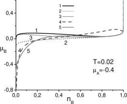
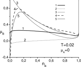
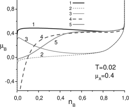
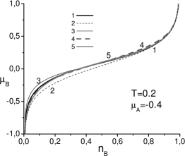
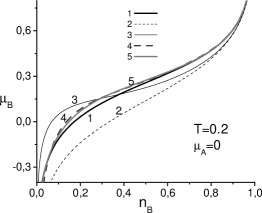
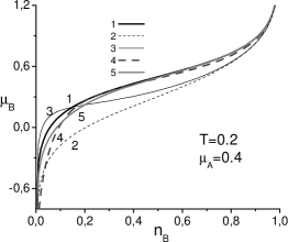
The dependence of the chemical potential on the concentration of localized particles is calculated using expressions (44), (50), (54), (55). In figure 4 the approximations such as AA, MAA, GH3 and H3 (in the last case the integral terms that describe the processes of scattering by boson excitations are neglected in the expressions for $R_{\sigma}$) are compared with the exact results obtained thermodynamically. The simple AA approximation cannot describe phase transitions because it gives a monotonically increasing dependence $\mu_{B}=\mu_{B}(n_{B})$. MAA and AA approximations can describe the thermodynamics of the system at high temperatures or at a negative value of $\mu_{A}$ (small concentration of moving particles). The H3 approximation gives better results for high temperatures but not for the low ones. The best results are given by the GH3 approximation for high temperatures, as well as for low temperatures in the cases of a nearly full or empty band of the moving particles (and high values of $n_{B}$).

Refer to caption
Refer to caption
Refer to caption
Refer to caption
Refer to caption
Refer to caption
Figure 5: $\mu_{B}$ as a function of $n_{B}$ in different approximations (1 – exact result; 2 – AA; 3 – MAA; 4 – H3; 5 – GH3) and corresponding densities of states $\rho_{B}$ of localized particles (1 – GH3; 2 – H3).

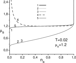
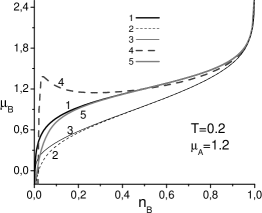
In figure 5 the case of a nearly full band of the moving particles is shown. The $\mu_{B}=\mu_{B}(n_{B})$ dependence is illustrated together with the corresponding curves for density of states of localized particles in H3 and GH3 approximations:

$$\rho_{B}(\omega)=-\frac{1}{\pi}\,\mathrm{Im}\,G_{B}^{(a)}(\omega+\mathrm{i}\varepsilon).$$ (56)

One can see that this band can have a complicated structure or even be split in the H3 approximation, but it does not correspond to the satisfactory $\mu_{B}(U_{B})$ dependence. In general, there is a considerable difference between densities of states $\rho_{B}(\omega)$ given by the H3 and GH3 approximations, but the band edges are determined properly even in the H3 approximation.

In figure 6 the densities of states of localized particles are presented for different temperatures and particle concentrations. In the cases corresponding to the above-mentioned criteria ((i) high $T$; (ii) low $T$ and chemical potential $\mu_{A}$ close to the edges of the band of the moving particles), the obtained densities of states $\rho_{B}$ can be considered as close to the real ones due to a satisfactory description of the $\mu_{B}(n_{B})$ dependences.

Refer to caption
Refer to caption
Refer to caption
Refer to caption
Refer to caption
Refer to caption
Figure 6: The approximate densities of states of localized particles (1 – GH3; 2 – H3).

Calculation of densities of states of localized particles in the Falicov-Kimball model had been done earlier within DMFT in [9, 10]. The algorithm which leads to exact results is rather complicated. The plots obtained in [9, 10] correspond to finite values of $U$ and to the symmetrical case of half-filling (the hypercubic lattice with Gaussian density of states was considered). The band of localized particles is split and consists of two subbands for $U$ larger than some critical value ($U\gtrsim 5~{}W_{A}$); for $U\rightarrow+\infty$, the only lower subband remains. Our results correspond by the general shape of the curves to the above-mentioned results in the cases illustrated in figure 5 for $T=0.02\;\ 0.2$; $\mu_{A}=1.2$; $n_{B}=0.9$ and in figure 6 for $T=0.2$; $\mu_{A}=0$; $n_{B}=0.9$ within the GH3 approximation (in these cases, there is the best agreement with the exact results for $\mu_{B}(n_{B})$ dependences). Quantitative comparison of densities of states of localized particles will be possible after doing calculations with nonperturbed density of state like in [9, 10] and for finite values of $U$.

6 Conclusions

Application of the approximate analytical method of solving the effective single-site problem within DMFT gives a basic set of equations for evaluating single-particle Green’s functions and for investigating an energy spectrum of the asymmetric Hubbard model describing the system of particles of two types with different transfer parameters ($t^{A}\neq t^{B}$) on a lattice.

The limiting case $U=\infty$ (exclusion of a double occupation of a site) and $t^{B}\rightarrow 0$ (the case of the infinitesimally small mobility of particles of one of the type, when the model becomes the Falicov-Kimball model) is considered.

Phase transitions are investigated in thermodynamic regimes of the fixed values of the following quantities: (i) $\mu_{A}$, $\mu_{B}$; (ii) $\mu_{A}$, $n_{B}$; or (iii) $\mu_{B}$, $n_{A}$. Phase diagrams describing coexistence curves of homogeneous phases with different $n_{A}$ and $n_{B}$ values and phase separation regions are obtained. These results extending a space of thermodynamic parameters complement the existing information about the thermodynamics of the Falicov-Kimball model in the $U\rightarrow+\infty$ limit.

The set of self-consistent equations, which relates the concentrations (chemical potentials) of particles of $A$ and $B$ types, coherent potentials $J_{A,B}(\omega)$ and shift constants of energy spectrum $\varphi_{A,B}$, is solved in two cases: (i) with an application of the exact thermodynamic relations for the Falicov-Kimball model to derive an equation for concentration $n_{B}$ of localized particles; (ii) by using the approximate analytical scheme in DMFT. Calculation of $\mu_{B}(n_{B})$ dependences being done by the two mentioned methods allows us to investigate an applicability of this approximate approach. The results closest to the exact ones are obtained within the GH3 approximation for high temperatures, as well as for low temperatures in the cases of nearly full or nearly empty band of the moving particles and for high values of $n_{B}$.

Densities of states $\rho_{B}(\omega)$ of localized particles are calculated using the approximate DMFT scheme. The results obtained in the GH3 approximation can be considered as the closest to the real ones, when a satisfactory dependence of $\mu_{B}(n_{B})$ is achieved. Extending this approach to the cases of low temperatures and intermediate band filling requires an improvement of the applied scheme, namely, a more precise (probably self-consistent) way of taking into account the processes of scattering by boson excitations for calculating the $R_{B}(\omega)$ function which determines the energy spectrum of localized particles.

Acknowledgements

This work was partially supported by the Fundamental Researches Fund of the Ministry of Ukraine of Science and Education (Project No. 02.07/266).

References

  • 1. Gruber Ch. Falicov-Kimball models: a partial review of the ground states problem. Preprint of arXiv.org e-Print archive, cond-mat/9811299, 1998, 18 p.
  • 2. Batista C.D. // Phys. Rev. Lett., 2002, vol. 89, p. 166403.
  • 3. Metzner W., Vollhardt D. // Phys. Rev. Lett., 1989, vol. 62, p. 324.
  • 4. Georges A., Kotliar G., Krauth W., Rosenberg M.J. // Rev. Mod. Phys., 1996, vol. 68, p. 13.
  • 5. Metzner W. // Phys. Rev. B, 1991, vol. 43, p. 8549.
  • 6. Brandt U., Mielsch C. // Z. Phys. B, 1989, vol. 75, p. 365; 1990, vol. 79, p. 295; 1991, vol. 82, p. 37.
  • 7. Freericks J.K. // Phys. Rev. B, 1999, vol. 60, p. 1617.
  • 8. Letfulov B.M. // Eur. Phys. J. B, 1999, vol. 11, p. 423–428.
  • 9. Brandt U., Urbanek M.P. // Z. Phys. B, 1992, vol. 89, p. 297–303.
  • 10. Zlatic V., Freericks J.K., Lemanski R., Czycholl G. // Philosophical Magazine B, 2001, vol. 81, p. 1443–1467.
  • 11. Stasyuk I.V. // Condens. Matter Phys., 2000, vol. 3, p. 437–456.
  • 12. Stasyuk I.V., Shvaika A.M. // Ukrainian Journal of Physics, 2002, vol. 47, p. 975.
  • 13. Tserkovnikov Yu.A. // Teor. Mat. Fiz., 1971, vol. 7, p. 260
  • 14. Plakida N.M. // Phys. Lett. A, 1973, vol. 43, p. 471
  • 15. Plakida N.M. Method of two-time Green’s functions in the theory of anharmonic crystals. – In: Statistical Physics and Quantum Field Theory, Ed. by Bogolyubov N.N., Moscov, 1973, p. 205–240.
  • 16. Potthoff M., Herrmann T., Wegner T., Nolting W. // Phys. Stat. Sol. (b), 1998, vol. 210, p. 199.
  • 17. Herrmann T., Nolting W. // Rhys. Rev. B, 1996, vol. 53, p. 10579.
  • 18. Falicov L.M., Kimball J.C. // Phys. Rev. Lett., 1969, vol. 22, p. 997.
  • 19. Letfulov B.M. // Eur. Phys. J. B, 1998, vol. 4, p. 447–457.
  • 20. Freericks J.K., Zlatic V. Exact solution of the Falicov-Kimball model with dynamical mean-field theory. Preprint of arXiv.org e-Print archive, cond-mat/0301188, 2003, 51 p.
  • 21. Stasyuk I.V., Shvaika A.M. // J. Phys. Studies, 1999, vol. 3, p. 177–183.
  • 22. Stasyuk I.V., Shvaika A.M. // Condens. Matter Phys., 1994, vol. 3, p. 133
  • 23. Stasyuk I.V., Shvaika A.M., Tabunshchyk K.V. // Condens. Matter Phys., 1999, vol. 2, p. 109
  • 24. Stasyuk I.V., Danyliv O.D. // Phys. Stat. Sol. (b), 1999, vol. 219, p. 299.