Lipid membranes with free edges

Abstract

Lipid membrane with freely exposed edge is regarded as smooth surface with curved boundary. Exterior differential forms are introduced to describe the surface and the boundary curve. The total free energy is defined as the sum of Helfrich’s free energy and the surface and line tension energy. The equilibrium equation and boundary conditions of the membrane are derived by taking the variation of the total free energy. These equations can also be applied to the membrane with several freely exposed edges. Analytical and numerical solutions to these equations are obtained under the axisymmetric condition. The numerical results can be used to explain recent experimental results obtained by Saitoh et al. [Proc. Natl. Acad. Sci. 95, 1026 (1998)].

I introduction

Theoretical study on shapes of closed lipid membranes made great progress two decades ago. The shape equation of closed membranes was obtained in 1987 oy1 , with which the biconcave discoidal shape of the red cell was naturally explained oy2 , and a ratio of $\sqrt{2}$ of the two radii of a torus vesicle membrane was predicted oy3 and confirmed by experiment Mutz .

During the formation process of the cell, either material will be added to the edge or the edge will heal itself so as to form closed structure. There are also metastable cup-like equilibrium shapes of lipid membranes with free edges Boal . Recently, opening-up process of liposomal membranes by talin Hotani ; Hotani2 has also been observed gives rise to the interest of studying the equilibrium equation and boundary conditions of lipid membranes with free exposed edges. Capovilla et al. first study this problem and give the equilibrium equation and boundary conditions Capovilla . They also discuss the mechanical meaning of these equations Capovilla ; Capovilla2 .

The study of these cup-like structures enables us to understand the assembly process of vesicles. Jülicher et al. suggest that a line tension can be associated with a domain boundary between two different phases of an inhomogeneous vesicle and leads to the budding Lipowsky . For simplicity, however, we will restrict our discussion on open homogenous vesicles.

In this paper, a lipid membrane with freely exposed edge is regarded as a differentiable surface with a boundary curve. Exterior differential forms are introduced to describe the surface and the curve. The total free energy is defined as the sum of Helfrich’s free energy and the surface and line tension energy. The equilibrium equation and the boundary conditions of the membrane are derived from the variation of the total free energy. These equations can also be applied to the membrane with several freely exposed edges. This is another way to obtain the results of Capovilla et al. Some solutions to the equations are obtained and the corresponding shapes are shown. They can be used to explain some known experimental results Hotani .

This paper is organized as follows: In Sec.II, we retrospect briefly the surface theory expressed by exterior differential forms. In Sec.III, we introduce some basic properties of Hodge star $\ast$. In Sec.IV, we construct the variational theory of the surface and give some useful formulas. In Sec.V, we derive the equilibrium equation and boundary conditions of the membrane from the variation of the total free energy. In Sec.VI, we suggest some special solutions to the equations and show their corresponding shapes. In Sec.VII, we put forward a numerical scheme to give some axisymmetric solutions as well as their corresponding shapes to explain some experimental results. In Sec.VIII, we give a brief conclusion and prospect the challenging work.

II surface theory expressed by exterior differential forms

In this section, we retrospect briefly the surface theory expressed by exterior differential forms. The details can be found in Ref.chen .

We regard a membrane with freely exposed edge as a differentiable and orientational surface with a boundary curve $C$, as shown in Fig.1. At every point on the surface, we can choose an orthogonal frame $\mathbf{e}_{1},\mathbf{e}_{2},\mathbf{e}_{3}$ with $\mathbf{e}_{i}\cdot\mathbf{e}_{j}=\delta_{ij}$ and $\mathbf{e}_{3}$ being the normal vector. For a point in curve $C$, $\textbf{e}_{1}$ is the tangent vector of $C$.

An infinitesimal tangent vector of the surface is defined as

$$d\mathbf{r}=\omega_{1}\mathbf{e}_{1}+\omega_{2}\mathbf{e}_{2},$$ (1)

where $d$ is an exterior differential operator, and $\omega_{1},\omega_{2}$ are 1-differential forms. Moreover, we define

$$d\mathbf{e}_{i}=\omega_{ij}\mathbf{e}_{j},$$ (2)

where $\omega_{ij}$ satisfies $\omega_{ij}=-\omega_{ji}$ because of $\mathbf{e}_{i}\cdot\mathbf{e}_{j}=\delta_{ij}$.

With $dd=0$ and $d(\omega_{1}\wedge\omega_{2})=d\omega_{1}\wedge\omega_{2}-\omega_{1}\wedge d\omega_{2}$, we have

$$d\omega_{1}=\omega_{12}\wedge\omega_{2};\quad d\omega_{2}=\omega_{21}\wedge\omega_{1};\quad\omega_{1}\wedge\omega_{13}+\omega_{2}\wedge\omega_{23}=0;$$ (3)

and

$$d\omega_{ij}=\omega_{ik}\wedge\omega_{kj}\quad(i,j=1,2,3),$$ (4)

where the symbol “$\wedge$” represents the exterior product on which the most excellent expatiation may be the Ref.arnold .

Eq.(3) and Cartan lemma imply that:

$$\omega_{13}=a\omega_{1}+b\omega_{2},\quad\omega_{23}=b\omega_{1}+c\omega_{2}.$$ (5)

Therefore, we have

$$\texttt{area element: }dA=\omega_{1}\wedge\omega_{2},$$ (6)

$$\texttt{first fundamental form: }I=d\mathbf{r}\cdot d\mathbf{r}=\omega_{1}^{2}+\omega_{2}^{2},$$ (7)

$$\texttt{second fundamental form: }II=-d\mathbf{r}\cdot d\mathbf{e}_{3}=a\omega_{1}^{2}+2b\omega_{1}\omega_{2}+c\omega_{2}^{2},$$ (8)

$$\texttt{mean curvature: }H=\frac{a+c}{2},$$ (9)

$$\texttt{Gaussian curvature: }K=ac-b^{2}.$$ (10)

III Hodge star $\ast$

In this part, we briefly introduce basic properties rather than the exact definition of Hodge star $\ast$ westenholz because we just use these properties in the following contents.

If $g,h$ are functions defined on 2D smooth surface $M$, then the following formulas are valid:

$$\ast f=f\omega_{1}\wedge\omega_{2};$$ (11)

$$\ast df=-f_{2}\omega_{1}+f_{1}\omega_{2},\quad if\quad df=f_{1}\omega_{1}+f_{2}\omega_{2};$$ (12)

$$d\ast df=\nabla^{2}f,\quad\nabla^{2}\texttt{ is the Laplace-Beltrami operator}.$$ (13)

We can easily prove that

$$\iint_{M}(fd\ast dg-gd\ast df)=\oint_{\partial M}(f\ast dg-g\ast df)$$ (14)

through Stokes’s theorem and integration by parts.

IV variational theory of the surface

the variation of the surface is defined as:

$$\delta\mathbf{r}=\Omega_{2}\mathbf{e}_{2}+\Omega_{3}\mathbf{e}_{3},$$ (15)

where the variation along $\mathbf{e}_{1}$ is unnecessary because it gives only an identity. Furthermore, let

$$\delta\mathbf{e}_{i}=\Omega_{ij}\mathbf{e}_{j},\quad\Omega_{ij}=-\Omega_{ji}.$$ (16)

Operators $d$ and $\delta$ are independent, thus $d\delta=\delta d$. $d\delta\mathbf{r}=\delta d\mathbf{r}$ implies that:

$$\delta\omega_{1} = \Omega_{2}\omega_{21}+\Omega_{3}\omega_{31}-\omega_{2}\Omega_{21},$$ (17)

$$\delta\omega_{2} = d\Omega_{2}+\Omega_{3}\omega_{32}-\omega_{1}\Omega_{12},$$ (18)

$$d\Omega_{3} = \Omega_{13}\omega_{1}+\Omega_{23}\omega_{2}-\Omega_{2}\omega_{23}.$$ (19)

Furthermore, $d\delta\mathbf{e}_{i}=\delta d\mathbf{e}_{i}$ implies that:

$$\delta\omega_{ij}=d\Omega_{ij}+\Omega_{ik}\omega_{kj}-\omega_{ik}\Omega_{kj}.$$ (20)

It is necessary to point out that the properties of the operator $\delta$ are exactly similar to those of the ordinary differential.

V equilibrium equation of the membrane and boundary conditions

The total free energy $F$ of a membrane with an edge is defined as the sum of Helfrich’s free energyhelfrich ; oy4 $F_{H}=\iint[\frac{k_{c}}{2}(2H+c_{0})^{2}+\bar{k}K]dA$ and the surface and line tension energy $F_{sl}=\lambda\iint dA+\gamma\oint_{C}ds$. Here $k_{c}$, $\bar{k}$, $c_{0}$, $\lambda$ and $\gamma$ are constants. With the arc-length parameter $ds=\omega_{1}$, the geodesic curvature $k_{g}=\omega_{12}/ds$ on $C$ and the Gauss-Bonnet formula $\iint KdA=2\pi-\oint_{C}k_{g}ds$, the total free energy and its variation are given

$$F=\iint[\frac{k_{c}}{2}(2H+c_{0})^{2}+\lambda]\omega_{1}\wedge\omega_{2}+\gamma\oint_{C}\omega_{1}-\bar{k}\oint_{C}\omega_{12}+2\pi\bar{k},$$ (21)

and

$$\delta F = k_{c}\iint(2H+c_{0})\delta(2H)\omega_{1}\wedge\omega_{2}+\iint[\frac{k_{c}}{2}(2H+c_{0})^{2}+\lambda]\delta(\omega_{1}\wedge\omega_{2})$$ (22)

$$+ \gamma\oint_{C}\delta\omega_{1}-\bar{k}\oint_{C}\delta\omega_{12},$$

respectively. From Eqs.(17) and (18), we can easily obtain:

$$\delta(\omega_{1}\wedge\omega_{2}) = \delta\omega_{1}\wedge\omega_{2}+\omega_{1}\wedge\delta\omega_{2}=-d(\Omega_{2}\omega_{1})-(2H)\Omega_{3}\omega_{1}\wedge\omega_{2}.$$ (23)

Eqs.(5), (17), (18) and (20) lead to:

$$\delta(2H)\omega_{1}\wedge\omega_{2} = \delta(a+c)\omega_{1}\wedge\omega_{2}$$ (24)

$$= 2(2H^{2}-K)\Omega_{3}\omega_{1}\wedge\omega_{2}+d(\Omega_{13}\omega_{2}-\Omega_{23}\omega_{1})$$

$$+ a\Omega_{2}d\omega_{1}-bd\Omega_{2}\wedge\omega_{2}+b\Omega_{2}d\omega_{2}+cd\Omega_{2}\wedge\omega_{1}.$$

Thus we have:

$$\delta F = k_{c}\iint(2H+c_{0})[2(2H^{2}-K)\Omega_{3}\omega_{1}\wedge\omega_{2}+d(\Omega_{13}\omega_{2}-\Omega_{23}\omega_{1})$$ (25)

$$+a\Omega_{2}d\omega_{1}-bd\Omega_{2}\wedge\omega_{2}+b\Omega_{2}d\omega_{2}+cd\Omega_{2}\wedge\omega_{1}]$$

$$+\iint(\frac{k_{c}}{2}(2H+c_{0})^{2}+\lambda)[-d(\Omega_{2}\omega_{1})-(2H)\Omega_{3}\omega_{1}\wedge\omega_{2}]$$

$$+\gamma\oint_{C}[\Omega_{2}\omega_{21}+\Omega_{3}\omega_{31}-\omega_{2}\Omega_{21}]-\bar{k}\oint_{C}[d\Omega_{12}+\Omega_{13}\omega_{32}-\omega_{13}\Omega_{32}].$$

If $\Omega_{2}=0$, then $d\Omega_{3}=\Omega_{13}\omega_{1}+\Omega_{23}\omega_{2}$, $\ast d\Omega_{3}=-\Omega_{23}\omega_{1}+\Omega_{13}\omega_{2}$. On curve $C$, $\omega_{2}=0$, $\omega_{31}=-a\omega_{1}$, $\omega_{32}=-b\omega_{1}$, $\Omega_{3}|_{C}=\Omega_{3C}$. Thus Eq.(25) is reduced to

$$\delta F = \iint[k_{c}(2H+c_{0})(2H^{2}-c_{0}H-2K)-2\lambda H]\Omega_{3}\omega_{1}\wedge\omega_{2}$$ (26)

$$+ k_{c}\iint(2H+c_{0})d\ast d\Omega_{3}-\gamma\oint_{C}a\omega_{1}\Omega_{3}+\bar{k}\oint_{C}(b\Omega_{13}-a\Omega_{23})\omega_{1}$$

In terms of Eqs.(13) and (14), we have:

$$\iint(2H+c_{0})d\ast d\Omega_{3}=\oint_{C}(2H+c_{0})\ast d\Omega_{3}-\oint_{C}\Omega_{3}\ast d(2H+c_{0})+\iint\Omega_{3}\nabla^{2}(2H+c_{0})\omega_{1}\wedge\omega_{2}.$$

Using integration by parts and Stokes’s theorem, we arrive at $\oint_{C}b\Omega_{13}\omega_{1}=\oint_{C}bd\Omega_{3C}=-\oint_{C}\Omega_{3C}db$. Thus

$$\delta F = \iint[k_{c}(2H+c_{0})(2H^{2}-c_{0}H-2K)-2\lambda H+k_{c}\nabla^{2}(2H+c_{0})]\Omega_{3}\omega_{1}\wedge\omega_{2}$$ (27)

$$-\oint_{C}[k_{c}(2H+c_{0})+\bar{k}a]\Omega_{23}\omega_{1}-\oint_{C}\Omega_{3C}[k_{c}\ast d(2H+c_{0})+\gamma a\omega_{1}+\bar{k}db].$$

It follows that

$$k_{c}(2H+c_{0})(2H^{2}-c_{0}H-2K)-2\lambda H+k_{c}\nabla^{2}(2H)=0,$$ (28)

$$\left.[k_{c}(2H+c_{0})+\bar{k}a]\right|_{C}=0,$$ (29)

$$\left.[k_{c}\ast d(2H)+\gamma a\omega_{1}+\bar{k}db]\right|_{C}=0.$$ (30)

The mechanical meanings of the above three equations are: Eq.(28) is the equilibrium equation of the membrane; Eq.(29) is the moment equilibrium equation of points on $C$ around the axis $\mathbf{e}_{1}$; and Eq.(30) is the force equilibrium equation of points on $C$ along the direction of $\mathbf{e}_{3}$ Capovilla ; Capovilla2 . It is not surprising that Eq.(29) contains the factor $\bar{k}$ because it is related to the bend energy in Helfrich’s free energy. However, it is difficult to understand why $\bar{k}$ is also included in Eq.(30). In fact, the term $\bar{k}db$ in Eq.(30) represents the shear stress which also contributes to the bend energy in Helfrich’s free energy.

In fact, $a=k_{n}$ and $b=\tau_{g}$ are the normal curvature and the geodesic torsion of curve $C$, respectively, and $\ast d(2H)=-\mathbf{e}_{2}\cdot\nabla(2H)\omega_{1}$. Thus Eqs.(29) and (30) become

$$\left.[k_{c}(2H+c_{0})+\bar{k}k_{n}]\right|_{C}=0,$$ (31)

$$\left.[-k_{c}\mathbf{e}_{2}\cdot\nabla(2H)+\gamma k_{n}+\bar{k}\frac{d\tau_{g}}{ds}]\right|_{C}=0,$$ (32)

respectively.

If $\Omega_{3}=0$, then $d\Omega_{3}=\Omega_{13}\omega_{1}+\Omega_{23}\omega_{2}-\Omega_{2}\omega_{23}=(\Omega_{13}-b\Omega_{2})\omega_{1}+(\Omega_{23}-c\Omega_{2})\omega_{2}=0$. It leads to $\Omega_{13}=b\Omega_{2}$ and $\Omega_{23}=c\Omega_{2}$.

$$\delta F = k_{c}\iint(2H+c_{0})[a\Omega_{2}d\omega_{1}-bd\Omega_{2}\wedge\omega_{2}+b\Omega_{2}d\omega_{2}+cd\Omega_{2}\wedge\omega_{1}+d(\Omega_{13}\omega_{2}-\Omega_{23}\omega_{1})]$$ (33)

$$+\iint[\frac{k_{c}}{2}(2H+c_{0})^{2}+\lambda][-d(\Omega_{2}\omega_{1})]+\gamma\oint_{C}\Omega_{2}\omega_{21}-\bar{k}\oint_{C}K\Omega_{2}\omega_{1}.$$

Otherwise, $\omega_{13}=a\omega_{1}+b\omega_{2}$ implies that: $ad\omega_{1}+db\wedge\omega_{2}+2bd\omega_{2}-cd\omega_{1}=-da\wedge\omega_{1}$. Thus

$$a\Omega_{2}d\omega_{1}-bd\Omega_{2}\wedge\omega_{2}+b\Omega_{2}d\omega_{2}+cd\Omega_{2}\wedge\omega_{1}+d(\Omega_{13}\omega_{2}-\Omega_{23}\omega_{1})$$ (34)

$$= -d(a+c)\wedge\Omega_{2}\omega_{1}=-d(2H+c_{0})\wedge\Omega_{2}\omega_{1}\texttt{ ($c_{0}$ is a constant)}.$$

Therefore

$$\delta F = \oint_{C}[-\frac{k_{c}}{2}(2H+c_{0})^{2}\Omega_{2}\omega_{1}-\bar{k}K\Omega_{2}\omega_{1}-\lambda\Omega_{2}\omega_{1}+\gamma\Omega_{2}\omega_{21}].$$ (35)

It follows that:

$$\left.[\frac{k_{c}}{2}(2H+c_{0})^{2}+\bar{k}K+\lambda+\gamma k_{g}]\right|_{C}=0,$$ (36)

because of $\omega_{21}=-k_{g}\omega_{1}$ on $C$. This equation is the force equilibrium equation of points on $C$ along the direction of $\mathbf{e}_{2}$ Capovilla ; Capovilla2 .

Eqs.(28), (31), (32) and (36) are the equilibrium equation and boundary conditions of the membrane. They correspond to Eqs. (17), (60), (59) and (58) in Ref.Capovilla , respectively. In fact, these equations can be applied to the membrane with several edges also, because in above discussion the edge is a general edge. But it is necessary to notice the right direction of the edges. We call these equations the basic equations.

VI Special solutions to basic equations and their corresponding shapes

In this section, we will give some special solutions to the basic equations together with their corresponding shapes. For convenience, we consider the axial symmetric surface with axial symmetric edges. Zhou has considered the similar problem in his PhD thesis zhou . If expressing the surface in 3-dimensional space as $\mathbf{r}=\{v\cos u,v\sin u,z(v)\}$ we obtain $2H=-(\frac{\sin\psi}{v}+\cos\psi\frac{d\psi}{dv})$, $K=\frac{\sin\psi\cos\psi}{v}\frac{d\psi}{dv}$, $\nabla(2H)=-\frac{\mathbf{r}_{2}}{\sec^{2}\psi}\frac{d}{dv}(\frac{\sin\psi}{v}+\cos\psi\frac{d\psi}{dv})$ and $\nabla^{2}(2H)=-\frac{\cos\psi}{v}\frac{d}{dv}[v\cos\psi\frac{d}{dv}(\frac{\sin\psi}{v}+\cos\psi\frac{d\psi}{dv})]$, where $\psi=\arctan[\frac{dz(v)}{dv}]$, $\mathbf{r}_{2}=\partial\mathbf{r}/\partial v$. Define $\mathbf{t}$ as the direction of curve $C$ and $\mathbf{r}_{1}=\partial\mathbf{r}/\partial u$. Obviously, $\mathbf{t}$ is parallel or antiparallel to $\mathbf{r}_{1}$ on curve $C$. Introduce a notation $sn$, such that $sn=+1$ if $\mathbf{t}$ is parallel to $\mathbf{r}_{1}$, and $sn=-1$ if not. Thus $\mathbf{e}_{2}=sn\frac{\mathbf{r}_{2}}{\sec\psi}$ and $\mathbf{e}_{2}\cdot\nabla(2H)=-sn\cos\psi\frac{\partial}{\partial v}(\frac{\sin\psi}{v}+\cos\psi\frac{d\psi}{dv})$ on curve $C$. For curve $C$, $k_{n}=-\frac{\sin\psi}{v}$, $\tau_{g}=0$, and $k_{g}=-sn\frac{\cos\psi}{v}$. Thus we can reduce Eqs.(28), (31), (32) and (36) to:

$$k_{c}(\frac{\sin\psi}{v} + \cos\psi\frac{d\psi}{dv}-c_{0})[\frac{1}{2}(\frac{\sin\psi}{v}+\cos\psi\frac{d\psi}{dv})^{2}+\frac{1}{2}c_{0}(\frac{\sin\psi}{v}+\cos\psi\frac{d\psi}{dv})-\frac{2\sin\psi\cos\psi}{v}\frac{d\psi}{dv}]$$ (40)

$$- \lambda(\frac{\sin\psi}{v}+\cos\psi\frac{d\psi}{dv})+k_{c}\frac{\cos\psi}{v}\frac{d}{dv}[v\cos\psi\frac{d}{dv}(\frac{\sin\psi}{v}+\cos\psi\frac{d\psi}{dv})]=0,$$

$$\left[k_{c}(\frac{\sin\psi}{v}+\cos\psi\frac{d\psi}{dv}-c_{0})+\bar{k}\frac{\sin\psi}{v}\right]_{C}=0,$$

$$\left[-sn\bar{k}\cos\psi\frac{d}{dv}(\frac{\sin\psi}{v})+\gamma\frac{\sin\psi}{v}\right]_{C}=0,$$

$$\left[\frac{\bar{k}^{2}}{2k_{c}}(\frac{\sin\psi}{v})^{2}+\bar{k}\frac{\sin\psi\cos\psi}{v}\frac{d\psi}{dv}+\lambda-sn\gamma\frac{\cos\psi}{v}\right]_{C}=0.$$

In fact, in above four equations only three of them are independent. We usually keep Eqs.(40), (40) and (40) for the axial symmetric surface. For the general case, we conjecture that there are also three independent equations among Eqs. (28), (31), (32) and (36). Eq.(40) is the same as the equilibrium equation of axisymmetrical closed membranes jghu ; seifert . In Ref seifert , a large number of numerical solutions to Eq.(40) as well as their classifications are discussed.

Next, Let us consider some analytical solutions and their corresponding shapes. We merely try to show that these shapes exist, but not to compare with experiments. Therefore, we only consider analytical solutions for some specific values of parameters.

VI.1 The constant mean curvature surface

The constant mean curvature surfaces satisfy Eq.(28) for proper values of $k_{c}$, $c_{0}$, $K$, and $\lambda$. But Eqs.(31), (32) and (36) imply $2H+c_{0}=0$, $k_{n}=0$, and $\bar{k}K+\gamma k_{g}=0$ on curve $C$ if $k_{c}$, $\bar{k}$, and $\gamma$ are nonzero.

For axial symmetric surfaces, $k_{n}=0$ requires $\sin\psi=0$. Therefore $K=0$ which requires $k_{g}=0$. Only straight line can satisfy these conditions. It contradicts to the fact that $C$ is a closed curve. Therefore, there is no axial symmetric open membrane with constant mean curvature.

VI.2 The central part of a torus

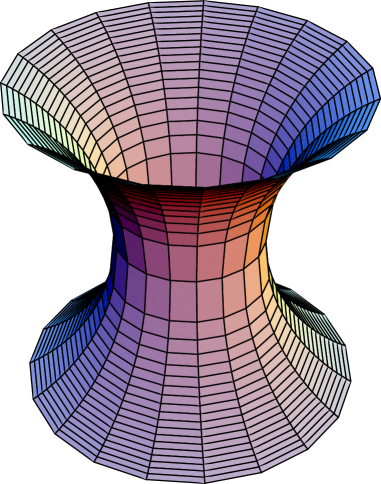
Figure 2: The central part of a torus.

When $\lambda=0$, $c_{0}=0$, the condition $\sin\psi=av+\sqrt{2}$ satisfies Eq.(40). It corresponds to a torus oy4 . Eqs.(40) and (40) determine the position of the edge $v_{e}=-\frac{\sqrt{2}(k_{c}+\bar{k})}{a(2k_{c}+\bar{k})}$, where $a=-\frac{\gamma(k_{c}+\bar{k})\sqrt{2(2k_{c}^{2}+4k_{c}\bar{k}+\bar{k}^{2})}}{(2k_{c}+\bar{k})k_{c}\bar{k}}$. If we let $k_{c}=\bar{k}$ and $\frac{k_{c}}{\gamma}=\frac{2\sqrt{14}}{3}\texttt{ (unit: length dimension)}$, it leads to $1/a=-1$ and $v_{e}=\frac{2\sqrt{2}}{3}\texttt{ (unit: length dimension)}$. Thus the shape is the central part of a torus as shown in Fig.2. This shape is topologically equivalent to a ring as shown in Fig.3.

VI.3 A cup

If we let $\sin\psi=\Psi$, according Hu’s method hu Eq.(40) reduce to:

$$(\Psi^{2}-1)\frac{d^{3}\Psi}{dv^{3}}+\Psi\frac{d^{2}\Psi}{dv^{2}}\frac{d\Psi}{dv}-\frac{1}{2}(\frac{d\Psi}{dv})^{3}+\frac{2(\Psi^{2}-1)}{v}\frac{d^{2}\Psi}{dv^{2}}+\frac{3\Psi}{2v}(\frac{d\Psi}{dv})^{2}$$

$$+(\frac{c_{0}^{2}}{2}+\frac{2c_{0}\Psi}{v}+\frac{\lambda}{k_{c}}-\frac{3\Psi^{2}-2}{2v^{2}})\frac{d\Psi}{dv}+(\frac{c_{0}^{2}}{2}+\frac{\lambda}{k_{c}}-\frac{1}{v^{2}})\frac{\Psi}{v}+\frac{\Psi^{3}}{2v^{3}}=0.$$ (41)

Now, we will consider the case that $\Psi=0$ for $v=0$. As $v\rightarrow 0$, Eq.(41) approaches to $\frac{d^{3}\Psi}{dv^{3}}+\frac{1}{v}\frac{d^{2}\Psi}{dv^{2}}-\frac{1}{v^{2}}\frac{d\Psi}{dv}+\frac{\Psi}{v^{2}}=0$. Its solution is $\Psi=\alpha_{1}/v+\alpha_{2}v+\alpha_{3}v\ln v$ where $\alpha_{1}=0$, $\alpha_{2}$ and $\alpha_{3}$ are three constants. If $\lambda=0$ and $c_{0}>0$, we find that $\Psi=\sin\psi=\beta(v/v0)+c_{0}v\ln(v/v_{0})$ satisfies Eq.(40). The shapes of closed membranes corresponding to this solution are fully discussed by Liu et al.liuqh . Eqs.(40) and (40) determine the position of the edge that satisfies $\tan\psi(v)=-\frac{\gamma}{2k_{c}c0}$ if $\bar{k}=-2k_{c}$. If let $\beta=1$, $v_{0}=1/c_{0}=1\texttt{ (unit: length dimension)}$ and $\gamma\gg k_{c}c_{0}$, we obtain $v/v_{0}\approx 1$ and its corresponding shape likes a cup as shown in Fig.4. This shape is topologically equivalent to a disk as shown in Fig.3.

VII axisymmetrical Numerical solutions

It is extremely difficult to find analytical solutions to Eq.(40). We attempt to find the numerical solutions in this section. But there is a difficulty that $\sin\psi(v)$ is multi-valued. To overcome this obstacle, we use the arc-length as the parameter and express the surface as $\mathbf{r}=\{v(s)\cos u,v(s)\sin u,z(s)\}$. The geometrical constraint and Eqs.(28), (31) and (36) now become:

$$v^{\prime}(s)=\cos\psi(s),\quad z^{\prime}(s)=\sin\psi(s),$$ (42)

$$(2-3\sin^{2}\psi)\psi^{\prime}v-\sin\psi(1+\cos^{2}\psi)+[(c_{0}^{2}+2\lambda/k_{c})\psi^{\prime}-(\psi^{\prime})^{3}-2\psi^{\prime\prime\prime}]v^{3}$$

$$\qquad+[(c_{0}^{2}+2\lambda/k_{c})\sin\psi-4c_{0}\sin\psi\psi^{\prime}+3\sin\psi(\psi^{\prime})^{2}-4\cos\psi\psi^{\prime\prime}]v^{2}=0,$$ (43)

$$\left[k_{c}(c_{0}-\frac{\sin\psi}{v}-\psi^{\prime})-\bar{k}\frac{\sin\psi}{v}\right]_{C}=0,$$ (44)

$$\left[\bar{k}c_{0}\frac{\sin\psi}{v}-\bar{k}(1+\frac{\bar{k}}{2k_{c}})\frac{\sin^{2}\psi}{v^{2}}+\lambda-sn\gamma\frac{\cos\psi}{v}\right]_{C}=0.$$ (45)

We can numerically solve Eqs.(42) and (43) with initial conditions $v(0)=0$, $\psi(0)=0$, $\psi^{\prime}(0)=\alpha$ and $\psi^{\prime\prime}(0)=0$ and then find the edge position through Eqs.(44) and (45). The shape corresponding to the solution is topologically equivalent to a disk as shown in Fig.3. In fact, Eq.(43) can be reduce to a second order differential equation Capovilla ; Capovilla2 ; zheng , but we still use the third order differential equation (43) in our numerical scheme.

In Fig.5, we depicts the outline of the cup-like membrane with a wide orifice. The solid line corresponds to the numerical result with parameters $\alpha=c_{0}=0.8\mu m^{-1}$, $\lambda/k_{c}=0.08\mu m^{-2}$, $\gamma/k_{c}=0.20\mu m^{-1}$ and $\bar{k}/k_{c}=0.38$. The squares come from Fig.1d of Ref.Hotani .

In Fig.6, we depicts the outline of the cup-like membrane with a narrow orifice. The solid line corresponds to the numerical result with parameters $\alpha=c_{0}=0.86\mu m^{-1}$, $\lambda/k_{c}=0.26\mu m^{-2}$, $\gamma/k_{c}=0.36\mu m^{-1}$ and $\bar{k}/k_{c}=-0.033$. The squares come from Fig.3k of Ref.Hotani .

Obviously, the numerical results agree quite well with the experimental results of Ref.Hotani .

VIII conclusion

In above discussion, we introduce exterior differential forms to describe a lipid membrane with freely exposed edge. The total free energy is defined as the Helfrich’s free energy plus the surface and line tension energy. The equilibrium equation and boundary conditions of the membrane are derived from the variation of the total free energy. These equations can also be applied to the membrane with several freely exposed edges. A numerical scheme to give some axisymmetric solutions and their corresponding shapes do agree with some experimental results.

The method that combines exterior differential forms with the variation of surface is of important mathematical significance. It is easy to be generalized to deal with and to simplify the difficult variational problems on high-dimensional manifolds.

Although we give some axisymmetric numerical solutions that agree with experimental results obtained by Saitoh et al, up to now, we still cannot find any unsymmetrical solution. A large number of unsymmetrical shapes are found in experiments, which will be a challenge to the theoretical study.

IX ACKNOWLEDGMENTS

We are grateful to the instructive advice of Mr. J. J. Zhou, H. J. Zhou, R. Capovilla and J. Guven. We thank Prof. Y. Z. Xie and Dr. L. Q. Ge for their critical reading our manuscript.

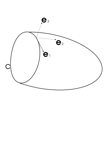
Figure 1: The surface with an edge $C$. At every point of the surface, we can construct an orthogonal frame $\mathbf{e}_{1},\mathbf{e}_{2},\mathbf{e}_{3}$, where $\mathbf{e}_{3}$ is the normal vector of the surface. For a point on curve $C$, $\textbf{e}_{1}$ is the tangent vector of $C$.

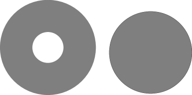
Figure 3: A ring (left) and a disk (right).

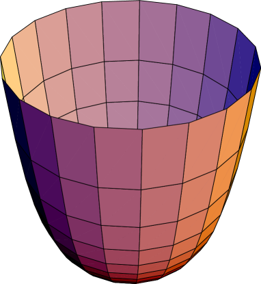
Figure 4: A cup.

Figure 5: The outline of the cup-like membrane with a wide orifice. The solid line is the numerical result with parameters $\alpha=c_{0}=0.8\mu m^{-1}$, $\lambda/k_{c}=0.08\mu m^{-2}$, $\gamma/k_{c}=0.20\mu m^{-1}$ and $\bar{k}/k_{c}=0.38$. The squares come from Fig.1d of Ref.Hotani . $z$-axis is the revolving axis and $v$ is the revolving radius.

Figure 6: The outline of the cup-like membrane with a narrow orifice. The solid line is the numerical result with parameters $\alpha=c_{0}=0.86\mu m^{-1}$, $\lambda/k_{c}=0.26\mu m^{-2}$, $\gamma/k_{c}=0.36\mu m^{-1}$ and $\bar{k}/k_{c}=-0.033$. The squares come from Fig.3k of Ref.Hotani . $z$-axis is the revolving axis and $v$ is the revolving radius.