Quantum gas-liquid condensation in an attractive Bose gas

Abstract

Gas-liquid condensation (GLC) in an attractive Bose gas is studied on the basis of statistical mechanics. Using some results in combinatorial mathematics, the following are derived: (1) With decreasing temperature, the Bose-statistical coherence grows in the many-body wave function, which gives rise to the divergence of the grand partition function prior to Bose-Einstein condensation. It is a quantum-mechanical analogue to the GLC in a classical gas (quantum GLC). (2) This GLC is triggered by the bosons with zero momentum. Compared with the classical GLC, an incomparably weaker attractive force creates it. For the system showing the quantum GLC, we discuss a cold helium 4 gas at sufficiently low pressure.

I Introduction

Gas-liquid condensation (GLC) is one of the universal phenomena occurring both in the classical and the quantum world. GLC is regarded as a singularity appearing in the pressure-volume curve determined by the equation of state:

$$\par\frac{P}{k_{B}T}=\lim_{V\to\infty}\frac{\ln Z_{V}(\mu)}{V},\par$$ (1)

$$\frac{\rho}{k_{B}T}=\lim_{V\to\infty}\frac{\partial}{\partial\mu}\left(\frac{\ln Z_{V}(\mu)}{V}\right).$$ (2)

The question is whether the grand partition function $Z_{V}(\mu)$ shows the singularity may yan . In ordinary GLC such as vapor condensation to water, the GLC occurs at relatively high temperature compared with the quantized energy. Hence, this GLC belongs to the classical phenomenon.

When GLC occurs at low temperature as in helium gas, however, the situation is different. One must seriously take into account the influence of quantum statistics on the GLC. In this paper, we call such a GLC quantum gas-liquid condensation to emphasize the key role quantum mechanics plays in the phenomenon, and we study its peculiar nature.

A prototype of the quantum GLC is the GLC in an attractive Bose gas at sufficiently low temperature. For the relationship between the GLC and Bose statistics, it has been often discussed in connection with Bose-Einstein condensation (BEC) hua . The following points, however, should be noted. (1) No BEC gas with an attractive interaction remains stable in thermal equilibrium. (The velocity of sound propagating through the condensate becomes imaginary bog .) (2) Since one of the two phases does not exist in the BEC phase, a transition between them is impossible. (3) Rather, the quantum GLC occurs in the normal phase close to the BEC transition point . In this region, the coherent many-body wave function is composed of many Bose particles, but it does not yet reach a macroscopic size. With decreasing temperature, the bosons’ kinetic energy approaches zero, but they do not experience a repulsive force until their distance reaches the hard-core radius. When a weak attractive force acts on such bosons, its influence is drastic. A dilute Bose gas will undergo GLC prior to BEC sto . Its remarkable difference from classical GLC is that, under the influence of Bose statistics, a negligibly weak interaction, which plays almost no role in the classical phenomenon, causes drastic changes of the system.

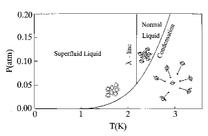
Figure 1: The phase diagram of helium 4 at low pressure. (In the inset, the wavy lines and the dotted lines around particles schematically represent the wave function and the zero-point motion, respectively.)

For the system showing the quantum GLC, we know an old example. At pressure lower than $0.05$ atm (triple point), a cold helium 4 gas in the normal phase undergoes a phase transition directly to a liquid in the superfluid phase as depicted in Fig.1 bri . At sufficiently low pressure, a gas is so rarefied that atoms experience a weak attractive interaction with distant atoms. Because of this weakness, the system remains in the gas state to such a temperature that its kinetic motion is affected by quantum statistics. Hence, it is probable that quantum statistics directly determines the character of this GLC wel .

An essential point to formulate the quantum GLC is that the coherent many-body wave function, which is symmetrical with respect to interchanges of a large number of particles, grows in $Z_{V}(\mu)$ at low temperature. At the vicinity of $T_{BEC}$ in the normal phase, it will give rise to the instability of the system. A precise formulation of this quantum effect is worth studying closely. The peculiar nature of Bose statistics manifests itself in momentum space. Hence, if one formulates the perturbation expansion of $Z_{V}(\mu)$ in momentum space, one may be able to obtain a straightforward expression of the instability. Along this line of thought, statistical mechanics of the quantum GLC was recently considered koh01 .

In this paper, using a different method from that in Ref.koh01 (see Appendix.A), we give a statistical-mechanical model of the quantum GLC . Mayer and others considered the divergence of the perturbation expansion of $Z_{V}(\mu)$ may . We will consider the quantum GLC along Mayer’s viewpoint koh03 . Using some results in combinatorial mathematics, we will derive a set of upper and lower bounds for $Z_{V}(\mu)$. By studying the radius of convergence for both bounds, we find that the divergence of $Z_{V}(\mu)$ occurs prior to BEC in cooling, which leads to the onset of the quantum GLC .

An outline of this paper is as follows. Sec.2 describes the Bose-statistical coherence appearing in $Z_{V}(\mu)$ at low temperature. Sec.3 develops a perturbation formalism of an attractive Bose gas along the viewpoint of Sec.2, and leads to the instability. Sec.4 compares the classical GLC with the quantum GLC , and discusses some differences between an attractive Bose and an attractive Fermi gas.

II Bose-statistical coherence

II.1 A model

We consider a spinless attractive Bose gas with a weakly attractive interaction $H_{it}$

$$H=\sum_{p}\epsilon_{p}a^{\dagger}_{p}a_{p}+U\sum_{p,p^{\prime},q}a^{\dagger}_{p-q}a^{\dagger}_{p^{\prime}+q}a_{p^{\prime}}a_{p},\quad(U<0).$$ (3)

The situation in a low-density gas, in which particles experience a negligibly weak interaction since they are far apart, and experience it only when a particle encounters other particles, enables us to use a contact interaction $U$. To characterize the initial stage of the instability occurring in a rarefied gas, we ignore the short-range repulsive force which plays an important role after the system reaches the high-density state. We regard $\sum_{p}\epsilon_{p}a^{\dagger}_{p}a_{p}$ as the unperturbed Hamiltonian, and obtain the grand partition function $Z_{V}(\mu)$=Tr $exp[-\beta(H-\mu N)]$ by the perturbation theory with respect to the interaction $H_{it}$

$$Z_{V}(\mu)=Z_{0}(\mu)\sum_{n=0}^{\infty}\frac{(-1)^{n}}{n!}$$ (4)

$$\times\int_{0}^{\beta}d\beta_{1}\cdots\int_{0}^{\beta}d\beta_{n}\langle TH_{it}(\beta_{1})\cdots H_{it}(\beta_{n})\rangle,$$

where $Z_{0}(\mu)$ is the grand partition function of an ideal Bose gas. ($(-1)^{n}$ comes from the Boltzmann factor.) The emergence of the Bose-statistical coherence appears not only in $Z_{0}(\mu)$ but also in $\langle TH_{it}(\beta_{1})\cdots H_{it}(\beta_{n})\rangle$.

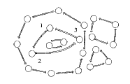
Figure 2: A pattern of elementary polygons in coordinate space, representing a set of permutations $P$ in the exponent of Eq.(8). The size of each polygon reflects a size of the coherent many-body wave function in $Z_{0}(\mu)$.

II.2 The unperturbed part $Z_{0}(\mu)$

Figure.2 schematically shows the coherent many-body wave functions in coordinate space. (Thick arrows represent permutation operations of Bose particles.) Matsubara mat and Feynman fey associated the grand partition function $Z_{0}(\mu)=\prod(1-e^{\beta(\epsilon_{p}-\mu)})^{-1}$ with such coherent wave functions as follows. The partition function $Z_{0}(N)$ of $N$ Bose particles is given by the density matrix $\rho(x_{1},\ldots x_{N};x_{1}^{\prime},\ldots x_{N}^{\prime};\beta)$ as tfey

$$Z_{0}(N)=\frac{1}{N!}\int\sum_{per}\rho(x_{1},\ldots x_{N};Px_{1},\ldots Px_{N};\beta)d^{N}x_{i},$$ (5)

where $P$ denotes permutations within $N$ particles, and $\rho$ is summed over all possible permutations. For the unperturbed part, the density matrix satisfying the “ideal gas” equation

$$\frac{\partial\rho}{\partial\beta}=\frac{\hbar^{2}}{2m}\sum_{i=1}^{N}\nabla^{2}_{i}\rho$$ (6)

has a form as

$$\rho(x_{1},\ldots x_{N};x_{1}^{\prime},\ldots x_{N}^{\prime};\beta)$$ (7)

$$=\left(\frac{m}{2\pi\beta\hbar^{2}}\right)^{3N/2}\exp\left[-\frac{m}{2\beta\hbar^{2}}\sum_{i}^{N}(x_{i}-x^{\prime}_{i})^{2}\right].$$

One therefore obtains

$$Z_{0}(N)=\frac{1}{N!}\left(\frac{m}{2\pi\beta\hbar^{2}}\right)^{3N/2}$$ (8)

$$\times\int\sum_{per}\exp\left[-\frac{m}{2\beta\hbar^{2}}\sum_{i}^{N}(x_{i}-Px_{i})^{2}\right]d^{N}x_{i}.$$

This expression of $Z_{0}(N)$ is interpreted as follows. For $N=3$ and $P=(1\rightarrow 2,2\rightarrow 3,3\rightarrow 1)$, the exponent of Eq.(8) includes $(x_{1}-x_{2})^{2}+(x_{2}-x_{3})^{2}+(x_{3}-x_{1})^{2}$. These permutations represent a triangle in Fig.2, which corresponds to a small coherent wave function. In general, the same particle appears only twice in $\Sigma(x_{i}-Px_{i})^{2}$ , first at an initial position $x_{i}$ and second at one of the final positions $Px_{i}$. The intermediate permutations between the initial and final $x_{s}$ form a closed graph, which is visualized as a polygon in Fig.2. As a result, one finds that many polygons are spreading out in coordinate space. (We call this an elementary polygon.) The size of the polygon (the number of its sides) corresponds to the number of particles, hence the size of the coherent wave function obeying Bose statistics (coherence size coh ). Each particle belongs to one of these polygons, and polygons do not share the same particle. A set of permutations in Eq.(8) corresponds to a pattern of polygons like Fig.2.

Ref.mat fey calculated $Z_{0}(N)$ by the following geometrical consideration. A polygon of size $s$ appears in the integrand in Eq.(8) as

$$\int\exp\left[-\frac{m}{2\beta\hbar^{2}}(x_{12}^{2}+\cdots+x_{s1}^{2})\right]d^{s}x_{i}\equiv f_{s}.$$ (9)

Assume a polygon distribution as $\{\xi_{1},\xi_{2},\ldots,\xi_{s},\ldots\}$, in which elementary polygons of size $s$ appear $\xi_{s}$ times, being subject to $N=\Sigma_{s}s\xi_{s}$. Consider the number of all configurations associated with $\{\xi_{s}\}$, and denote it with $B(\xi_{1},\ldots,\xi_{s},\ldots)$. One can rewrite Eq.(8) as

$$Z_{0}(N)=\frac{1}{N!}\left(\frac{m}{2\pi\beta\hbar^{2}}\right)^{3N/2}$$ (10)

$$\times\sum_{\{\xi_{s}\}}B(\xi_{1},\ldots,\xi_{s},\ldots)f_{1}^{\xi_{1}}\cdots f_{s}^{\xi_{s}}\ldots.$$

(1) $B(\xi_{1},\ldots,\xi_{s},\ldots)$ is estimated as follows fey . Assume $N$ particles in an array. The number of ways of partitioning them into $\{\xi_{s}\}$ is given by $N!/\Pi_{s}\xi_{s}!$. An array of $s$ particles corresponds to a polygon of size $s$. For the coherent wave function, it does not matter which particle is an initial one in the array (circular permutation). Hence, $N!/\Pi_{s}\xi_{s}!$ must be multiplied by a factor $1/s$ for each $\xi_{s}$, with a result that

$$B(\xi_{1},\ldots,\xi_{s},\ldots)=\frac{N!}{\prod_{s}\xi_{s}!s^{\xi_{s}}}.$$ (11)

With Eq.(11) in Eq.(10), one obtains

$$Z_{0}(N)=\frac{1}{\lambda^{3N}}\sum_{\{\xi_{s}\}}\prod_{s}\frac{f_{s}^{\xi_{s}}}{\xi_{s}!s^{\xi_{s}}},$$ (12)

where $\lambda=(2\pi\beta\hbar^{2}/m)^{1/2}$ is the thermal wavelength.

(2) Using Eq.(12), we obtain the grand partition function $Z_{0}(\mu)=\Sigma_{N}Z_{0}(N)e^{\beta\mu N}$, in which summation over $N$ changes to free summation over $\xi_{s}$ from $0$ to $\infty$. Substituting $N=\Sigma_{s}s\xi_{s}$ into $\lambda^{3N}$ in Eq.(12) and $e^{\beta\mu N}$ yields

$$Z_{0}(\mu)=\prod_{s}\exp\left[\frac{f_{s}}{s}\left(\frac{e^{\beta\mu}}{\lambda^{3}}\right)^{s}\right].$$ (13)

The $f_{s}$ in Eq.(9) is estimated with the convolution theorem (see Appendix.B), with which one obtains

$$Z_{0}(\mu)=\exp\left[\sum_{s=1}^{\infty}\left(\frac{e^{\beta\mu s}}{s}+A_{s}\frac{V}{\lambda^{3}}\frac{e^{\beta\mu s}}{s^{5/2}}\right)\right].$$ (14)

The first and the second term in the exponent come from $p=0$ and $p\neq 0$ bosons, respectively, both of which are expansions with respect to the coherence size $s$ as . Using

$$-\sum_{s=1}^{\infty}\frac{x^{s}}{s}=\ln(1-x),$$ (15)

and

$$\sum_{s=1}^{\infty}\frac{x^{s}}{s^{5/2}}=-\frac{4}{\sqrt{\pi}}\int_{0}^{\infty}y^{2}\ln(1-xe^{-y^{2}})dy,$$ (16)

Eq.(14) agrees with $Z_{0}(\mu)=\prod(1-e^{\beta(\epsilon_{p}-\mu)})^{-1}$.

Using Eq.(14) in Eq.(1), the coherent many-body wave function appears in the equation of states as follows:

$$\frac{P}{k_{B}T}=\lim_{V\to\infty}\frac{1}{V}\sum_{s}\frac{h(s)}{s},$$ (17)

where $h(s)$ is the size distribution of the coherent wave function ($1/s$ on the right-hand side is a geometrical factor.). In view of Eq.(14), one has $h(s)=e^{\beta\mu s}$ for $p=0$ and $h(s)=(A_{s}V/\lambda^{3})(e^{\beta\mu s}/s^{1.5})$ for $p\neq 0$. The chemical potential $\mu$ determines the size distribution. At high temperature ($\mu\ll 0$), $h(s)$ falls off exponentially with a size $s$, and large polygons are therefore negligible (Boltzmann statistics). With decreasing temperature ($\mu\rightarrow 0$), the exponential dependence on $s$ weakens as $e^{\beta\mu s}\rightarrow 1$, thus making large polygons significant. (At the BEC transition point, its size dependence disappears for $p=0$, and the macroscopic wave function therefore contributes to $Z_{0}(\mu)$ as much as the microscopic one.) It should be noted that, even in the normal phase, the large but not macroscopic coherent many-body wave functions exist at the vicinity of the BEC transition point, and make considerable contributions to the grand partition function.

II.3 $\langle TH_{it}(\beta_{1})\cdots H_{it}(\beta_{n})\rangle$

In an attractive Bose gas, we must extend the concept of Bose-statistical coherence from $Z_{0}(\mu)$ to $\langle TH_{it}(\beta_{1})\cdots H_{it}(\beta_{n})\rangle$ in Eq.(4).

At high temperature, relatively simple diagrams are significant in $\langle TH_{it}(\beta_{1})\cdots H_{it}(\beta_{n})\rangle$. A typical example in momentum space is the sum of ring diagrams composed of bubbles like Fig.3. A thin solid line with an arrow represents a boson propagator, and dotted lines denote the attractive interaction.

Assume that $\langle TH_{it}(\beta_{1})\cdots H_{it}(\beta_{n})\rangle$ is decomposed into $h_{1}+h_{2}+\cdots$ disconnected diagrams containing closed loops, in which each of $h_{1}$ diagrams contains $m_{1}$ interaction lines, each of $h_{2}$ diagrams contains $m_{2}$ interaction lines, and so on ($n=\sum_{i}h_{i}m_{i}$). The total number of such diagrams is $n!/h_{1}!h_{2}!\cdots$. A disconnected diagram with $m$ interaction lines contributes to $Z_{V}(\mu)$ as

$$\Xi_{m}=\frac{(-1)^{m}}{m!}$$ (18)

$$\times\int_{0}^{\beta}d\beta_{1}\cdots\int_{0}^{\beta}d\beta_{m}\langle TH_{it}(\beta_{1})\cdots H_{it}(\beta_{m})\rangle.$$

Hence, a sum of all disconnected diagrams

$$n!\sum_{h_{1}}\frac{1}{h_{1}!}\Xi_{1}^{h_{1}}\sum_{h_{2}}\frac{1}{h_{2}!}\Xi_{2}^{h_{2}}\cdots$$ (19)

replaces the multiple integrals with $(-1)^{n}$ in Eq.(4), and free sums over $h_{i}$ replace the sum over $n$ as

$$Z_{V}(\mu)=Z_{0}(\mu)\exp\left(\Xi_{1}+\Xi_{2}+\cdots\right).$$ (20)

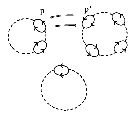
Figure 3: Some ring diagrams in momentum space, composed of bubbles of bosons (an example of $n$=7 terms in Eq.(4)). Dotted lines represent the attractive interaction in Eq.(3).

With decreasing temperature, the wave function in $\langle TH_{it}(\beta_{1})\cdots H_{it}(\beta_{n})\rangle$ becomes symmetrical with respect to interchanges of particles. The sum of rings in Fig.3 changes as follows: When one of two particles in one bubble and that of another bubble have the same momentum ($p=p^{\prime}$), an exchange of these particles by the thick arrows yields a square as in Fig.4, which links two small rings. The inclusion of such diagrams in $Z_{V}(\mu)$ ensures the principle of Bose statistics that many identical particles have the tendency to occupy the same state ($p=p^{\prime}$).

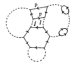
Figure 4: A polygon cluster including a square and a hexagon, which are made by exchanging particles between two bubbles and between three bubbles in Fig.3, respectively. It belongs to the $(2,1,1,0,0,0,0)$ pattern, an example of $K_{1}^{\nu_{1}}\cdots K_{s}^{\nu_{s}}$-type graphs.

Similarly, when three particles are exchanged between three bubbles in the lower part of Fig.3, a hexagon is yielded as in Fig.4. Further, when two particles are interchanged between the square and the hexagon in the cluster, a decagon is yielded. Such a sequence will continue to a single large polygon in Fig.5. Starting from $n$ bubbles, $n$ times of particle interchange between two bubbles leads to a single large polygon consisting of $2n$ bosons ($2n$ gon). The size of the polygons (the number of its sides) reflects the number of particles, hence the size of the coherent wave function. With decreasing temperature, the large coherent wave-function becomes important not only in $Z_{0}(\mu)$ but also in $\langle TH_{it}(\beta_{1})\cdots H_{it}(\beta_{n})\rangle$.

In the unperturbed part $Z_{0}(\mu)$, we consider the elementary polygons. Here, we find another type of polygon at each order of the perturbation. From now on we call this type of polygons an interaction polygon. Both polygons are different, complementary expressions of the coherent many-body wave function. In contrast with the elementary polygons, this type of polygon has an interaction line at each vertex, thus being connected with each other. As depicted in Fig.4, a $2s$-sized polygon is composed of $s$ bosons with $(p_{i},l_{i})$, and another $s$ bosons with $[-(p_{i}+q_{i}),-(l_{i}+m_{i})]$, with an expression given by

$$K_{s}=\prod_{i=1}^{s}U\frac{1}{\beta}$$

$$\times\left(\frac{1}{\displaystyle{(\epsilon_{p_{i}}-\mu)+i\frac{\pi l_{i}}{\beta}}}\frac{1}{\displaystyle{(\epsilon_{-(p_{i}+q_{i})}-\mu)-i\frac{\pi(l_{i}+m_{i})}{\beta}}}\right),$$

where $l,m$ is an even integer including zero. While the elementary polygons in $Z_{0}(\mu)$ represent a series of successive one-particle permutations like Fig.2, the interaction polygons represent intertwining of many permutations.

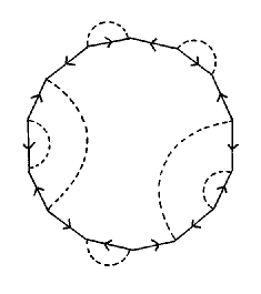
Figure 5: A single largest polygon (14-gon) as a final result of particle interchanges. It belongs to the $(0,0,0,0,0,0,1)$ pattern, an example of $K_{n}$-type graphs.

III Formalism

To formulate the concept of polygons in $\langle TH_{it}(\beta_{1})\cdots H_{it}(\beta_{n})\rangle$, it is useful to make reference to the description below Eq.(9). In a polygon cluster, let us assume a distribution of interaction polygons as $\{\nu_{s}\}=\{\nu_{1},\nu_{2},\ldots\}$, in which a polygon $K_{s}$ of size $2s$ appears $\nu_{s}$ times. (For example, $\{\nu_{s}\}=\{2,1,1,0,\ldots\}$ in Fig.4.) They are connected to each other by $n$ interaction lines, in which $2s$ interaction lines emerge from $2s$-sized polygon. Hence, $n=\sum_{s}s\nu_{s}$ must be satisfied.

Consider the number of all configurations corresponding to $\{\nu_{s}\}$, and denote it by $D_{n}(\nu_{1},\ldots,\nu_{s},\ldots)$. One can rewrite $\Xi_{n}$ in Eq.(20) with Eq.(18) in terms of interaction polygons as follows:

$$\Xi_{n}=V\frac{1}{n!}\sum_{\{\nu_{s}\}}D_{n}(\nu_{1},\ldots,\nu_{s},\ldots)K_{1}^{\nu_{1}}\cdots K_{s}^{\nu_{s}}\cdots,$$ (22)

which is the analogue of Eq.(10) for $Z_{0}(N)$. $H_{it}$ in Eq.(3) is a function of the distance between particles in coordinate space. When the integral in coordinate space is performed in $\langle TH_{it}(\beta_{1})\cdots H_{it}(\beta_{n})\rangle$, relative coordinates of particles are used, thus reducing multiplicity of the integral by one, with a further factor $V$ entering in the right-hand side of Eq.(22), which represents the translation of the polygon cluster .

For evaluating $\Xi_{n}$, one must consider the influence of Bose statistics on $\prod_{s}(K_{s})^{\nu_{s}}$ and make a graphical consideration of $D_{n}(\nu_{1},\ldots,\nu_{s},\ldots)$.

III.1 Effects of Bose statistics

In $\prod_{s}(K_{s})^{\nu_{s}}$ of Eq.(22), Bose statistics manifests itself in the following manner.

(1) With decreasing temperature, the feature of Bose statistics, accumulation of particles in the low-energy state, becomes apparent, thus making the bosons have a common momentum in each polygon. Hence, one assumes $p_{i}=p,l_{i}=l$, and $q_{i}=m_{i}=0$ in Eq.(21), which effectively restricts $U$ in Eq.(3) to the pairing-type interaction. Since each $K_{s}$ has its own $p$ and $l$ in Eq.(22), the summation must be done. One must sum up all cases by replacing each $K_{s}$ in Eq.(22) with $\sum_{l,p}K_{s}$. One therefore redefines $K_{s}$ in Eq.(22) as

$$K_{s}=\sum_{l,p}\left(-U\frac{1}{\beta}\frac{1}{\displaystyle{(\epsilon_{p}-\mu)^{2}+\left(\frac{\pi l}{\beta}\right)^{2}}}\right)^{s}\equiv\sum_{l,p}x(p,l)^{s}.$$ (23)

($(-1)^{m}$ in Eq.(18) is absorbed in a negative sign in front of $U$ in Eq.(23).)

(2) Let us compare the graph like Fig.4 ($K_{1}^{\nu_{1}}\cdots K_{s}^{\nu_{s}}$-type) and Fig.5 ($K_{n}$-type). Since each $K_{s}$ of $K_{1}^{\nu_{1}}\cdots K_{s}^{\nu_{s}}\cdots$ includes a sum over $p$ and $l$ as in Eq.(23), $\prod_{s}(K_{s})^{\nu_{s}}$ in Eq.(22) includes the multiple summation. Hence, the number of $K_{1}^{\nu_{1}}\cdots K_{s}^{\nu_{s}}$-type graphs is larger than that of a $K_{n}$-type graph. With decreasing temperature, however, the feature of Bose statistics, accumulation of particles in the low-energy state, reduces these degrees of freedom. At low temperature, all $K_{s}$ of $K_{1}^{\nu_{1}}\cdots K_{s}^{\nu_{s}}\cdots$ are likely to have a common $p$ and $l$. Hence, with decreasing temperature, the various $K_{1}^{\nu_{1}}\cdots K_{s}^{\nu_{s}}$ terms ($=[\sum x(p_{1},l_{1})]^{\nu_{1}}\cdots[\sum x(p_{s},l_{s})^{s}]^{\nu_{s}}$) approach a single form $K_{n}=\sum_{p,l}x(p,l)^{n}$, because of $n=\sum_{s}s\nu_{s}$.

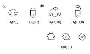
Figure 6: Polygon clusters. (a) For $n$=2, $D_{2}(2,0)=1$ and $D_{2}(0,1)=1$. (b) For $n$=3, $D_{3}(3,0,0)=1$, $D_{3}(1,1,0)=1$, and $D_{3}(0,0,1)=3$.

(3) In an attractive Bose gas ($U<0$), $K_{s}$ is always positive in Eq.(23), and $\Xi_{n}$ in Eq.(22) is therefore a positive-term series. Hence, to derive the upper and the lower bound for $\Xi_{n}$, one can take only large terms in Eq.(22) without considering the cancellation of terms. (For a repulsive Bose gas, the situation is different rep .)

III.2 Graphical consideration of a polygon cluster

For $D_{n}(\nu_{1},\ldots,\nu_{s},\ldots)$ in Eq.(22), it is useful to draw explicitly polygon clusters in some cases, and get a feeling for its magnitude. For $n=2,3,4$, we classify the distributions $\{\nu_{s}\}$ satisfying $n=\sum_{s}s\nu_{s}$, and we obtain some $D_{n}$’s as illustrated in Fig.6 and 7.

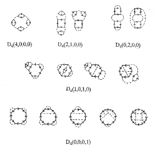
Figure 7: Polygon clusters for $n$=4: $D_{4}(4,0,0,0)=1$, $D_{4}(2,1,0,0)=2$, $D_{4}(0,2,0,0)=2$, $D_{4}(1,0,1,0)=4$, and $D_{4}(0,0,0,1)=5$.

$n=2$. For $\{\nu_{1},\nu_{2}\}$ satisfying $2=\nu_{1}+2\nu_{2}$, one has $\{2,0\}$ and $\{0,1\}$.

$n=3$. For $\{\nu_{1},\nu_{2},\nu_{3}\}$ satisfying $3=\nu_{1}+2\nu_{2}+3\nu_{3}$, one gets $\{3,0,0\}$,$\{1,1,0\}$ and $\{0,0,1\}$.

$n=4$. For $\{\nu_{1},\nu_{2},\nu_{3},\nu_{4}\}$ satisfying $4=\nu_{1}+2\nu_{2}+3\nu_{3}+4\nu_{4}$, one obtains $\{4,0,0,0\}$, $\{2,1,0,0\}$, $\{0,2,0,0\}$, $\{1,0,1,0\}$, and $\{0,0,0,1\}$.

Fig.6(a) shows $D_{2}(2,0)=1,D_{2}(0,1)=1$.

Fig.6(b) shows $D_{3}(3,0,0)=1$, $D_{3}(1,1,0)=1$ and $D_{3}(0,0,1)=3$.

Fig.7 shows $D_{4}(4,0,0,0)=1$, $D_{4}(2,1,0,0)=2$, $D_{4}(0,2,0,0)=2$, $D_{4}(1,0,1,0)=4$, and $D_{4}(0,0,0,1)=5$.

In view of Fig.6 and 7, one notices the following:

(1) In polygon clusters with $n$ interaction lines, there are many types of $\{\nu_{s}\}$ ranging from $\{n,0,\ldots,0\}$ to $\{0,\ldots,0,1\}$. From now on, we call a group of graphs with the same distribution $\{\nu_{s}\}$ a “pattern.” (For $n$=4, there are five patterns in Fig.7.) The number of patterns $p(n)$ appearing in the $n$ th-order graphs is equivalent to the number of ways of writing $n$ as a sum of positive integers ($n=\sum_{s}s\nu_{s}$). In combinatorial mathematics, this problem is known as “partition of $n$” han . It is known to have the following asymptotic form as $n\rightarrow\infty$:

$$p(n)\sim\frac{1}{4\sqrt{3}n}\exp\left(\pi\sqrt{\frac{2n}{3}}\right).$$ (24)

(2) At a given $n$, the pattern with the largest number of configurations $D_{n}$ consists of the largest polygons in size (the $2n$-gon, $\{0,\ldots,0,1\}$). We can confirm that this tendency becomes more evident as $n$ increases. From now on, we abbreviate $D_{n}(0,\ldots,0,1)$ as $D(n)$. (Fig.4 and 5 are examples of polygons with seven interaction lines. Due to various arrangements of dotted lines, there are more Fig.5-type graphs than Fig.4-type ones.)

Combining $p(n)$ and $D(n)$, one derives an inequality for $\Sigma D_{n}$ at a given $n$ in $n\rightarrow\infty$,

$$D(n)<\sum_{\{\nu_{s}\}}D_{n}(\nu_{1},\ldots,\nu_{s},\ldots)$$ (25)

$$<\frac{1}{4\sqrt{3}n}\exp\left(\pi\sqrt{\frac{2n}{3}}\right)D(n),$$

where the lower bound is a case in which the sum over $\{\nu_{s}\}$ in $\Sigma D_{n}$ includes only a pattern composed of the largest polygons, and the upper bound is a case in which all patterns at a given $n$ are included as if their $D_{n}$ is the same as $D(n)$ of the largest polygon.

(3) With decreasing temperature, large polygons, which are successively produced by particle interchanges between small polygons, become significant. Because the “pairing interaction” becomes significant for Bose statistics ($q_{i}=m_{i}=0$ in Eq.(21)), directions of arrows in such polygons are restricted. As shown in Fig.5, 6, and 7, there appear only special types of graphs, in which every two vertices connected by a dotted line are separated by odd (not even) number of sides. In combinatorial mathematics, the exact formula of $D(n)$ for such graphs was recently found nak , and it has the following asymptotic form (Appendix.C) per :

$$D(n)\rightarrow\frac{n!}{4n},\quad as\quad n\rightarrow\infty.$$ (26)

Substituting Eq.(26) into Eq.(25) yields an inequality for $\Sigma D_{n}$, which will be discussed below.

III.3 The instability of an attractive Bose gas in the normal phase

Let us obtain an inequality for $Z_{V}(\mu)$ in low temperature. Replacing $K_{1}^{\nu_{1}}\cdots K_{s}^{\nu_{s}}\cdots$ in Eq.(22) by $K_{n}$ (as stated in (2) of Sec.3.A), and using Eq.(25) with Eq.(26) in Eq.(22), one obtains

$$V\frac{1}{4n}K_{n}<\Xi_{n}<V\frac{1}{16\sqrt{3}n^{2}}\exp\left(\pi\sqrt{\frac{2n}{3}}\right)K_{n}.$$ (27)

Using Eq.(23) in $K_{n}$ of Eq.(27) and applying it to Eq.(20), one obtains con

$$Z_{0}(\mu)\prod_{p,l}\exp\left(V\sum_{n=1}^{\infty}\frac{1}{4n}x(p,l)^{n}\right)<Z_{V}(\mu)$$ (28)

$$<Z_{0}(\mu)\prod_{p,l}\exp\left(V\sum_{n=1}^{\infty}\frac{\exp\left(\pi\sqrt{\frac{2n}{3}}\right)}{16\sqrt{3}n^{2}}x(p,l)^{n}\right).$$

If the infinite series over $n$ in the exponent of the upper bound is convergent for all $p$ and $l$, it guarantees the finiteness of $Z_{V}(\mu)$, hence the stability of an attractive Bose gas. Cauchy-Hadamard’s theorem asserts that the radius of convergence $r_{c}$ of a power series $\sum_{n=1}^{\infty}a_{n}x^{n}$ is given by (see Appendix.D)

$$\frac{1}{r_{c}}=\lim_{n\to\infty}|a_{n}|^{1/n}.$$ (29)

Applying this theorem to the upper bound [$a_{n}=\exp(\pi\sqrt{\frac{2n}{3}})/(16\sqrt{3}n^{2})$] and the lower bound [$a_{n}=1/(4n)$] in Eq.(28), and using $\lim_{n\to\infty}n^{1/n}=1$, one obtains 1 as $r_{c}$’s of both bounds. Hence, $Z_{V}(\mu)$ has the radius of convergence $r_{c}=1$ as well. For each $p,l$, the convergence condition $x(p,l)<r_{c}$ is given by

$$-U\frac{1}{\beta}\frac{1}{(\epsilon_{p}-\mu)^{2}+\left(\frac{\pi l}{\beta}\right)^{2}}<1.$$ (30)

The equation of state (1) and (2) implicitly determines the chemical potential of a gas as a function of its temperature and pressure or density. At high temperature, $\mu\ll 0$ is satisfied for the regions in $P-\rho$ space, and Eq.(30) is therefore satisfied with respect to all $p$ and $l$. Hence, an attractive Bose gas ($U<0$) exists as the thermodynamically stable state.

With decreasing temperature, however, the negative $\mu$ gradually increases at a given $P$ or $\rho$. Changing $P,T$ or $\rho,T$ in $\mu$ of Eq.(30) makes possible the violation of the convergence condition. Among many $p$ and $l$, this condition is first violated at $p=l=0$ when $\mu$ reaches a certain critical value $\mu_{c}$ as

$$-\frac{U}{\beta\mu_{c}^{2}}=1,$$ (31)

where $\mu_{c}$ satisfies

$$\mu_{c}=-\sqrt{-Uk_{B}T_{c}}.$$ (32)

When $\mu$ reaches $\mu_{c}$, $Z_{V}(\mu)$ abruptly diverges without any precursory behavior. Hence the specific volume $v$, determined by

$$\frac{1}{v}=k_{B}T\lim_{V\to\infty}\frac{\partial}{\partial\mu}\left(\frac{\ln Z_{V}(\mu)}{V}\right),$$ (33)

discontinuously jumps to zero. This means that each particle cannot keep large distances from other particles. Hence an attractive Bose gas undergoes a transition to the high-density state.

The condensation point $(P_{c},\rho_{c})$ in the isothermal curve is determined by the equation of state and

$$\mu(\rho_{c},T)=-\sqrt{-Uk_{B}T}$$ (34)

at a given temperaturenee .

For considering the influence of attractive force on the coherent many-body wave function, its critical size is of great interest. Specifically, the critical size distribution $h(s)$ of elementary polygons in Sec.2B is a significant quantity gpl . At high temperature ($\mu\ll-k_{B}T$), $h(s)$ is a rapidly decreasing function of $s$. With decreasing temperature, $h(s)$ gradually changes to a weakly $s$-dependent distribution, finally reaching $h_{c}(s)$ at the condensation line

$$h_{c}(s)=\left\{\begin{array}[]{ll}\displaystyle{\exp\left(\frac{\mu_{c}}{k_{B}T_{c}}s\right)}&\qquad p=0\\[5.69046pt] \displaystyle{\frac{V}{\lambda^{3}}\frac{A_{s}}{s^{1.5}}\exp\left(\frac{\mu_{c}}{k_{B}T_{c}}s\right)}&\qquad p\neq 0,\end{array}\right.$$

beyond which distribution an attractive Bose gas does not exist in the gas phase. Hence, $h_{c}(s)$ is a critical size-distribution of the coherent many-body wave function in the gas phase.

The divergence of $Z_{V}(\mu)$ occurs first in bosons with zero momentum. This means that among many bosons with various momentums, the bosons with zero momentum escape first from a gas, and make a liquid droplet at a certain point of the gas. Since this droplet is a high-density boson with $p=0$, it is likely that the growth of this droplet leads to a liquid in the BEC phase. As stated in Sec.1, in thermal equilibrium a Bose gas in the BEC phase undergoes no GLC, whereas its GLC in the normal phase is likely to trigger the formation of the BEC condensate as a by-product. The GLC of a normal helium 4 gas to a superfluid liquid at $P<0.05$ atm falls into this category. (One finds a parallel on this point in the BCS transition, in which the formation of loosely bound pairs of fermions is promptly followed by the formation of their BEC condensate.)

III.4 Weak $U$ limit

In contrast with the classical GLC, the weak-coupling limit ($U\simeq 0$) is one of the realistic situations of the quantum GLC. Even if $-U$ is very small, the condition (34) is satisfied for a small $\mu$ at the vicinity of the BEC transition point in the normal phase. In principle, an arbitrarily weak attractive interaction creates the quantum GLC at sufficiently low temperature.

When we approximate $\mu$ in Eq.(34) with $\mu_{0}$ of an ideal Bose gas, we can make a rough estimation of $T_{c}$ and $\mu_{c}$ under the fixed density. In an ideal Bose gas, Eq.(2) is expanded as rob

$$\frac{\lambda^{3}}{v}=g_{3/2}(e^{\beta\mu})\simeq 2.612-3.545\sqrt{|\beta\mu(T)|},$$ (35)

where $g_{a}(x)=\sum_{n}x^{n}/n^{a}$. Using Eq.(34) in $\mu(T)$ of the right-hand side of Eq.(35) at $T_{c}$, and dividing both sides with $\lambda_{0}^{3}/v=2.612$ (an ideal Bose gas), one obtains

$$\left(\frac{\beta_{c}}{\beta_{0}}\right)^{1.5}+1.36\sqrt[4]{\frac{-U}{k_{B}T_{0}}}\left(\frac{\beta_{c}}{\beta_{0}}\right)^{0.25}-1=0.$$ (36)

At $U\simeq 0$, one gets

$$T_{c}\simeq T_{0}\left[1+0.90\sqrt[4]{\frac{-U}{k_{B}T_{0}}}\right],$$ (37)

and

$$\mu_{c}\simeq-\sqrt{-Uk_{B}T_{0}}\left[1+0.45\sqrt[4]{\frac{-U}{k_{B}T_{0}}}\right].$$ (38)

($T_{0}$ denotes the BEC transition temperature of an ideal Bose gas at the same $\rho$ eqr .)

Figure.8 shows a schematic phase diagram. The dotted curve depicts the $P-T_{0}$ curve of an ideal Bose gas, $P=(m/2\pi\hbar^{2})^{1.5}g_{5/2}(1)(k_{B}T_{0})^{2.5}$. The solid curve illustrates the $P-T_{c}$ curve (condensation line) derived by applying Eq.(37) to the $P-T_{0}$ curve. As a crude estimation of $T_{BEC}$ (traced back to London), we use $\lambda^{3}/v=g_{3/2}(1)$ with the experimental value of liquid density, and get $k_{B}T_{BEC}=2\pi\hbar^{2}m^{-1}2.612^{-1/3}(N/V)^{1/3}$. In Fig.8, the solid curve and a straight line $T=T_{BEC}$ intersect at the triple point. This schematic diagram is useful only for conceptual understanding, and comparing it with the phase diagram of the helium 4 needs elaborate calculations of some quantities, especially of the liquid state.

IV Discussion

IV.1 Comparison with the classical GLC

In the phase diagram of helium 4 like Fig.1, with increasing pressure, the nature of the GLC continuously changes from the quantum to the classical GLC cri . Let us compare the classical and the quantum GLC. Since this paper considers only the attractive interaction for the quantum GLC, we can make comparison only on the initial stage of the instability. In the classical GLC, Mayer’s method considers the singularity which must appear in the perturbation expansion of $Z_{V}(\mu)=\Sigma a_{n}x^{n}$. In general, the relationship between the coefficient $a_{n}$ and the interaction potential is so complicated that it is a difficult problem whether the $a_{n}$ derived from a given potential actually leads to such a singularity gro .

(a) In a classical gas, since the GLC occurs at relatively high temperature, the inelastic scattering is important. Hence, one must perform an $(s-1)$-dimensional integral for obtaining the cluster integral. In the GLC of a dilute Bose gas, however, since it occurs at very low temperature, the diagram with a common momentum $p$ like Fig.5 becomes important. Hence, the integrals of a $2s$-sized polygon are factorized, and the bounds for $Z_{V}(\mu)$ become simple as in Eq.(28).

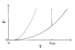
Figure 8: A schematic phase diagram. The dotted curve is the $P-T_{0}$ curve of an ideal Bose gas at the BEC point. The solid curve is the condensation line, that is, the $P-T_{c}$ curve obtained by applying Eq.(37) to the $P-T_{0}$ curve.

(b) In a classical gas, one can prove the convergence or the divergence of $Z_{V}(\mu)$ only after summing up all momentum components. In an attractive Bose gas, however, the instability is expected to occur at bosons with zero momentum. Hence, one can prove the divergence of $Z_{V}(\mu)$ by focusing on the $p=0$ component of $\Xi_{n}$.

(c) In the classical GLC, due to the absence of Bose statistics, there are far more $K_{1}^{\nu_{1}}\cdots K_{s}^{\nu_{s}}$-type clusters than $K_{n}$-type polygons. Hence, at each order of the perturbation, one cannot estimate $Z_{V}(\mu)$ only by the largest polygons in size. For the quantum GLC, however, one can estimate $Z_{V}(\mu)$ by focusing the largest polygons as in Sec.3.B.

These features (a) $\sim$ (c) will become useful for elucidating the essence of the quantum GLC and studying the classical-quantum crossover of the GLC in future studies.

IV.2 The quantum GLC in fermions

There is another type of quantum GLC occurring in fermions such as a helium 3 gas. In the phase diagram of helium 3, the location of the normal-superfluid transition in the liquid phase is far apart from the condensation line between the liquid and the gas phase. (This is in contrast with helium 4 in Fig.1.) Hence, it is uncertain to what extent the observed GLC is affected by Fermi statistics wel . In principle, however, the quantum GLC in fermions has some different features from that in bosons. For an ideal Fermi gas, due to one-particle excitation, the antisymmetrical coherent wave functions are not formed even at zero temperature, whereas it shows the Cooper instability with the attractive force. Hence, it is appropriate to begin with the pairing interaction when considering the GLC. In a Fermi gas, a similar argument to that in Sec.2.C is valid as well: When two Fermi particles ($p$ and $p^{\prime}$) belonging to two different bubbles have the same momentum ($p=p^{\prime}$), a new diagram containing a square must be included with a negative sign gau lan . Its $K_{s}$ has a similar form to Eq.(23) except for an odd integer $l$, and $\Xi_{n}$ of an attractive Fermi gas has a similar structure to Eq.(22) in appearance. But the argument in Sec.3.A is affected by Fermi statistics as follows.

(a) Due to Fermi statistics, each $K_{s}$ in Eq.(22) has its own momentum and frequency even at zero temperature, and the number of the $K_{1}^{\nu_{1}}\cdots K_{s}^{\nu_{s}}$-type cluster is therefore larger than that of the $K_{n}$-type polygon in $\Xi_{n}$. Hence, at a given $n$, dominant terms in the perturbation series do not come from the $K_{n}$-type polygon, but from the various $K_{1}^{\nu_{1}}\cdots K_{s}^{\nu_{s}}$-type polygon clusters. (In n=7 for example, the polygon cluster like Fig.4 is more important than the single largest polygon like Fig.5.) In this respect, the GLC in a Fermi gas has the same feature as the classical GLC [see (c) in Sec.4.A].

(b) For Fermi statistics, a negative sign appears in front of $U$ in $K_{s}$ (Eq.(21)), because of $a^{\dagger}_{p}a^{\dagger}_{-p}a_{-p^{\prime}}a_{p^{\prime}}=-a^{\dagger}_{p}a_{-p^{\prime}}a^{\dagger}_{-p}a_{p^{\prime}}$ for $p\neq p^{\prime}$. Accordingly, the negative sign in front of $U$ ($<0$) in Eq.(23) disappears. Hence, $\Xi_{n}$ of an attractive Fermi gas is an alternating series. The perturbation series of an attractive Fermi gas has a completely different structure from that of an attractive Bose gas. That is, one must consider the cancellation of terms which are opposite in sign, and cannot approximate $\Xi_{n}$ only by the terms with large $D_{n}$. One must carefully count all $K_{1}^{\nu_{1}}\cdots K_{s}^{\nu_{s}}$-type clusters in Eq.(22). Gaudin gau and Langer lan gave an approximation of $Z_{V}(\mu)$ along this line of thought, and led the BCS gap equation from it. (Using their result, a rigorous proof was given recently that, as long as attractive force is increased within the BCS scheme, the GLC is impossible koh97 .) Application of the inequality method to an attractive Fermi gas is a future problem.

IV.3 Future problems

Lastly, we point out some problems in future studies of the quantum GLC .

(a) For Mayer’s method of condensation, we know a long-standing problem in the interpretation of results. Since this method focuses on the instability of a gas and contains no information on a liquid, there remains a question whether the singularity of the power series in $Z_{V}(\mu)$ actually gives the condensation temperature $T_{c}$, or corresponds to an end point of supersaturation $T_{s}$. This problem is related with technical difficulties in estimating the grand partition function. In general, it is difficult to treat the highly inhomogeneous system so that it will reach true thermal equilibrium. Poor approximations of $Z_{V}(\mu)$ often include the uniform-density restraint, thus preventing the system from reaching true thermal-equilibrium. The singularity of $Z_{V}(\mu)$ obtained by such an approximation corresponds to the end point of supersaturation. If a satisfactory approximation is made, it will lead to the condensation point in thermal equilibrium. Hence, the validity of Mayer’s method depends on the type of phenomenon. For bosons, we can have the following optimistic view: The uniformity of the system by $p=0$ particles is the characteristic property of bosons at low temperature. Hence the satisfactory approximation of $Z_{V}(\mu)$ is more probable than that of more inhomogeneous systems. A quantitative analysis of this point is a future problem. In this paper, we used the term “$T_{c}$ of the GLC” as a generic name for the temperature at which a Bose gas shows the instability leading to the collapse.

(b) To discuss a liquid on a common basis with a gas, one must make a more realistic model by including the short-range repulsive interaction into Eq.(3). In this case, one must expect interference of the attractive $U$ and the repulsive $U^{\prime}$ in $\Xi_{n}$, with a result that $\Xi_{n}$ becomes intermediate between the positive-term series and the alternating series. An estimation of such a series is a difficult problem.

(c) For the classical GLC, there appears long-range correlation at the vicinity of the condensation point, which comes from the general mechanism of a first-order phase transition. For the quantum GLC in an attractive Bose gas, the long-range coherence comes from Bose statistics. This difference may affect the nature of fluctuations in the vicinity of a transition point.

(d) The recent experiment of trapped atomic Bose gas will provide us with a new tool par . Ultralow temperature is available and direct control of the effective interparticle force becomes possible using magnetic field. The system of interest from our viewpoint is not a BEC gas, but a normal gas just above the BEC transition point dil . The trapped atomic Bose gas, however, has its own properties which may complicate the foregoing arguments, that is, metastability. The confinement of atoms by a harmonic potential gives rise to the spatial inhomogeneity in the system. Many bosons gather at the center of a trap. The resulting increased density enhances the zero-point motion of particles, which stabilizes the gas state. For a trapped atomic Bose gas with attractive interaction, one finds a metastable BEC state at low temperature and below critical density. Up to now, the collapse of such a metastable BEC gas was detected bra cor , but the GLC in the normal phase has not been observed. Further, there is a possibility that a state after the transition is not a liquid but a solid or molecules. If it is true, we must consider this system from a different viewpoint.

Appendix A Comments on Ref.[8]

As a starting point to $Z_{V}(\mu)$ of an attractive Bose gas, Ref.koh01 began with an approximate formula [Eq.(9) in Ref.koh01 ], which carefully deals with the $K_{1}^{\nu_{1}}\cdots K_{s}^{\nu_{s}}$-type cluster like Fig4. As confirmed in Sec.3, however, the peculiar nature of a Bose gas appears in the $n\rightarrow\infty$ limit. In this limit, Eq.(9) and all subsequent integrals (with respect to $t$) in Ref.koh01 turn out to diverge. The finial form of $Z_{V}(\mu)$ (Eq.(21) in Ref.koh01 ) approaches $\infty-\infty$, which loses the mathematical meaning. Hence, it is questionable to identify it as a Yang-Lee zero. (One way to avoid this divergence is to perform all integrals in Ref.koh01 over $[0,M]$ with a finite $M$ instead of $[0,\infty]$. But such a trick is unnatural in a Bose gas.) In this paper, we prove the singularity of $Z_{V}(\mu)$ by showing its divergence using the inequality; this gives a sound basis to the instability condition (Eq.(34)), which was first obtained in Ref.koh01 .

Appendix B polygons in $Z_{0}(\mu)$

$f_{s}$ in Eq.(9) is estimated as follows fey . If $x_{s1}^{2}$ [the last term in the exponent of Eq.(9)] is replaced by $x_{s0}^{2}$, $f_{s}$ becomes a function of $x_{1}-x_{0}(\equiv x_{10})$ as $f_{s}(x_{10})$. Equation (9) shows that $f_{s}(x_{10})$ is made by $(s-1)$ times of the convolution of $\exp(-mx^{2}/2\beta\hbar^{2})$. Hence, using its three-dimensional Fourier transform $\Gamma(p)=\lambda^{\prime 3}\exp(-\lambda^{\prime 2}p^{2}/2)$, where $\lambda^{\prime}=\lambda/\sqrt{2\pi}$, $f_{s}(x_{10})$ is expressed as

$$f_{s}(x_{10})=\frac{V}{(\sqrt{2\pi})^{3}}\int(\sqrt{2\pi})^{3(s-1)}\Gamma(p)^{s}e^{-ipx_{10}}4\pi p^{2}dp,$$ (39)

where $V$ corresponds to the translation of the elementary polygons. Since $f_{s}=f_{s}(x_{10}=0)$, one has

$$f_{s}=V\int(\sqrt{2\pi})^{3s}\Gamma(p)^{s}\frac{4\pi p^{2}dp}{(2\pi)^{3}}.$$ (40)

After extracting $\Gamma(p=0)$ from the integrand of Eq.(B2) and performing the integral, one obtains

$$f_{s}=\left(\lambda^{3s}+A_{s}\lambda^{3(s-1)}\frac{V}{s^{3/2}}\right).$$ (41)

Appendix C asymptotic formula of $D$

The asymptotic form of $D(n)$ (Eq.(26)) is derived as follows nak . We think of regular $2n$-polygons with $n$ interaction lines, in which $n$ lines connect $n$ pairs of vertices separated by an odd number of sides. We denote its number by $D(n)$, and classify it by a transformation property such as rotation and reflection: A polygon is invariant under rotations through angle $\pi l/n$ ($l=0,1,\ldots,2n-1$). Further, a $2n$-polygon is symmetrical with respect to the $2n$ axis. Hence the symmetry group is composed of $4n$ elements $C_{0},C_{1},\ldots,C_{4n-1}$. We denote by $\phi(C_{i})$ the number of graphs which are invariant under transformation $C_{i}$.

Birnside’s theorem liu states $D(n)=\Sigma\phi(C_{i})/4n$. The most important $\phi(C_{i})$ is the number of polygons invariant under an identical transformation $\phi(C_{0})=n!$ (the number of ways of connecting $n$ pairs of vertices). Among many $\phi(C_{i})$’s, the $\phi(C_{0})$ becomes dominant as $n\rightarrow\infty$. Hence, taking only $\phi(C_{0})$ in $\Sigma\phi(C_{i})$, one obtains an asymptotic form $D(n)\rightarrow n!/4n$ at $n\rightarrow\infty$.

For $D(n)$ with a finite $n$, one must classify $2n$-polygons with interaction lines by symmetry, and include other $\phi(C_{i})$’s in $\Sigma\phi(C_{i})$. The result is as follows nak .

Theorem 1 (Nakamura)

The number of the nonequivalent 1-regular odd spanning subgraphs of the complete graph of order 2n by the Dihedral group $D_{2n}$ is given by

$$D(n)=\frac{n!}{4n}+\frac{1}{4n}\sum_{i=1}^{2n-1}R^{2n}_{i}+\frac{1}{4}(S_{0}+S_{1}),$$

where

$$R_{i}^{2n}=\left\{\begin{array}[]{ll}\displaystyle{0},&\quad d=odd,n=2m\\ \\[5.69046pt] \displaystyle{\sum_{d=2s+t}\frac{d!}{2^{s}s!t!}\left(\frac{n}{d}\right)^{s}},&\quad d=odd,n=2m+1\\ \\[5.69046pt] \\ \displaystyle{\left(\frac{2n}{d}\right)^{d/2}\left(\frac{d}{2}\right)!},&\quad d=even,\end{array}\right.$$

(d is the greatest common divisor of 2n and i, and s and t are positive).

$$S_{0}=\left\{\begin{array}[]{ll}\displaystyle{0},&\quad n=2m\\[5.69046pt] \displaystyle{2^{(n-1)/2}\left(\frac{n-1}{2}\right)!},&\quad n=2m+1,\end{array}\right.$$

$$S_{1}=\sum_{n=2s+t}\frac{n!}{2^{s}s!t!}\quad.$$

Appendix D Cauchy-Hadamard’s theorem

We begin with a general series $\sum_{n=1}^{\infty}c_{n}$. If one can find $k$ and $m$ such that $\sqrt[n]{c_{n}}\leq k<1$ when $n\geq m$, one gets for a large $n$

$$S_{n}=c_{1}+\cdots+c_{n}<k+\cdots+k^{n}=\frac{k(1-k^{n})}{1-k}.$$ (42)

Since $0<k<1$, $\sum_{n=1}^{\infty}c_{n}$ converges.

The above result is used in $\sum_{n=1}^{\infty}a_{n}x^{n}$ with $|a_{n}x^{n}|$ identified as $c_{n}$. By defining $\lim_{n\rightarrow\infty}|a_{n}|^{1/n}\equiv l$, one obtains $\lim_{n\rightarrow\infty}|a_{n}x^{n}|^{1/n}=l|x|$, that is, $\lim_{n\rightarrow\infty}\sqrt[n]{c_{n}}=l|x|$.

This means that, if $l|x|<1$, Eq.(D1) is valid, hence $\sum_{n=1}^{\infty}c_{n}$ converges. Contrarily, if $l|x|>1$, it diverges. The radius of convergence $r_{c}$ of $\sum_{n=1}^{\infty}a_{n}x^{n}$ is given by $l|r_{c}|=1$, that is,

$$\frac{1}{r_{c}}=\lim_{n\to\infty}|a_{n}|^{1/n}.$$ (43)

References

- (1) J.E.Mayer and M.G.Mayer, Statistical Mechanics (John Wiely and Sons, New York, 1946), B.Kahn and G.E.Uhlenbeck, Physica 5,399 (1938), M.Born and K.Fuchs, Proc.Roy.Soc (London) A166,391 (1938)
- (2) C.N.Yang and T.D.Lee, Phys.Rev, 87,404(1952).
- (3) As an early reference, K.Huang, Phy.Rev,119,1129(1960)
- (4) N.N.Bogoliubov, J.Phys.USSR, 11,23(1947)
- (5) H.T.Stoof, Phy.Rev.A,49,3824(1994).
- (6) F.G.Brickwedde, H.van Dijk, M.Durieux,J.R.Clement and J.K.Logan, J.Res.NBS, 64A, 1(1960).
- (7) At 1 atm, however, the GLC of a helium 4 gas to a normal liquid is regarded as the classical GLC (). At 1 atm, the interaction between helium atoms is not so weak that the GLC occurs at relatively high temperature, thus washing out the feature of quantum statistics. (A helium 3 gas at 1 atm undergoes the GLC at . The small difference of between 4He and 3He suggests that quantum statistics plays a minor role.)
- (8) S.Koh, Phy.Rev.B,64,134529(2001).
- (9) Since there are some subtle points in Mayer’s model of condensation, we confine ourselves to general features of quantum GLC without referring to controversial points. A preliminary report is S.Koh, Phyica.B, 329-333,(2003) 38.
- (10) T.Matsubara, Prog.Theo.Phys.6, 714 (1951).
- (11) R.P.Feynman, Phys.Rev. 90, 1116 (1953), ibid 91, 1291 (1953). (The interaction is considered within elementary polygons in Ref.mat , and in the effective mass in Ref.fey . These treatments are for the repulsive force, and not sufficient for the attractive one.)
- (12) For example, R.P.Feynman, Statistical Mechanics, (Addison-Wesley, 1972).
- (13) Note that the coherence size is a different concept from the coherence length (healing length).
- (14) For a weakly -dependent factor , see Ref.mat
- (15) In a repulsive Bose gas (), the sign of alternates as increases. Hence Eq.(22) becomes an alternating series, making the estimation of perturbation series difficult.
- (16) For example, Handbook of discrete and combinatorial mathematics, K.H.Rosen.ed, 115 (CRC press, 2000).
- (17) O.Nakamura, Scientiae.Mathematicae.Japonicae, 59, 463 (2004).
- (18) After one of is fixed in , making all possible permutations of operators yields (circular permutation), which agrees with the order of at in Eq.(26).
- (19) Both bounds have a form of , which must approach at as generally proved in Ref.yan .
- (20) Since the BEC phase is excluded from a list of possible states of an attractive gas in thermal equilibrium, there is no need to compare Eq.(34) with the BEC condition.
- (21) In addition to , the size distribution of interaction polygons is another important quantity, and we denote it by . It appears in the pressure of a gas as . In contrast with , many ’s with different are connected to each other in the logarithm. Hence, is not as simple as .
- (22) J.E.Robinson, Phy.Rev,83,678(1951).
- (23) Equation (32) in Ref.koh01 must be replaced by Eq.(38) in this paper.
- (24) The critical point (the end point of the condensation line) is an attribute of the classical GLC.
- (25) For a few models, more elaborate analysis of has been made. As a review, J.Groeneveld, 229, in Graphical Theory and Theoretical Physics, F.Hararry.ed, (Academic press, London and NewYork, 1967).
- (26) M.Gaudin, Nucl.Phys.A,20,513(1960).
- (27) J.S.Langer, Phys.Rev.A, 134,553(1964). (The sign definition of in of Ref. gau lan is different from ours.)
- (28) S.Koh, Phys.Lett.A, 229,59(1997)
- (29) As a review, A.S.Parkins and D.F.Walls, Phy.Rep, 303, 1 (1998), F.Dalfovo, S.Giorgini, L.P.Pitaevskii and S.Stringari, Rev.Mod,71, 463(1999), A.Leggett, Rev.Mod.Phys,73, 307(2001).
- (30) In a low-density gas, the different wave functions overlap only slightly. At the vicinity of the BEC phase, however, the emergence of the large coherent many-body wave function completely changes the situation. In fact, a trapped atomic BEC gas cooled by optical techniques is times as dilute as the measurable low-pressure limit of helium 4 gas cooled by the conventional method.
- (31) C.C.Bradley, C.A.Sackett, J.J.Tollett and R.G.Hulet, Phys.Rev.Lett, 75,1687(1995)
- (32) S.L.Cornish, N.R.Claussen, J.L.Roberts, E.A.Cornell and C.E.Wieman, Phys.Rev.Lett, 85, 1795 (2000).
- (33) For example, C.L.Liu, Introduction to Combinatorial Mathematics, (McGraw-Hill, 1968).