Transition from Type-I to Type-II Superconducting Behaviour with Temperature observed by $\mu$SR and SANS

Abstract

We investigate the superconducting behaviour of Bi doped Pb. Pure lead shows type-I behaviour entering an intermediate state in a magnetic field. High dopings of Bi ($>$3$\%$) lead to type-II behaviour showing a mixed state, where the magnetic field penetrates the superconductor in the form of a flux lattice. At intermediate doping, the sample shows both type-I and type-II behaviour depending on the temperature. This arises because the Ginzburg-Landau parameter $\kappa$ passes through its critical value of $1/\sqrt{2}$ with temperature.

I INTRODUCTION

When a superconductor is brought into a magnetic field, its behaviour depends on the balance of its fundamental length scales. The first of these, the penetration depth $\lambda$, describes the length over which the applied field penetrates into the superconductor. The second, the coherence length $\xi$, roughly gives the spatial extent of the Cooper pair. Phenomenologically, $\xi$ marks the length scale over which the macroscopic wave function of the supercarriers varies. In the treatment of superconductors by Ginzburg and Landau, this wavefunction takes the role of the order parameter in the Landau theory of phase transitions. The ratio of the two length scales, $\kappa=\lambda/\xi$, determines the response of the superconductor to an applied magnetic field. In the case that $\kappa<1/\sqrt{2}$, the superconductor is said to be of type-I. Such a type-I superconductor will expel a magnetic field completely, apart from a layer at the surface of thickness $\lambda$. This is true as long as the field is smaller than some critical field $B_{c}$, associated with the de-pairing current. For applied fields higher than $B_{c}$, superconductivity is lost and the field penetrates a sample like a normal metal. The region of the thermodynamic B-T phase diagram below $B_{c}$, in which the superconductor behaves as an ideal diamagnet is also called the Meissner-state. If the sample geometry is such that there are sizable demagnetising effects, even a small applied field will exceed the critical field the edges of the sample [2]. At these places the field will be able to penetrate the superconductor. As a result, normal conducting regions with a penetrating field of $B_{c}$, and superconducting regions in the Meissner state (expelling the field) will coexist in the sample. This state is called the intermediate state. To minimise the surface energy of these coexisting domains, the normal state-patches form an irregular pattern, similar to that of Weiss-domains found in ferromagnets.

In addition to the Meissner-state, a type-II superconductor (with $\kappa>1/\sqrt{2}$) shows a second superconducting phase, in which it is energetically more favourable for the field to penetrate the sample in the form of quantised vortices of magnetic flux. These flux lines mutually repell and form a regular lattice, that is usually of hexagonal symmetry. This second superconducting phase consists of the mixed state, where the whole of the sample makes up a vortex lattice. The mixed state extends up to a field $B_{c_{2}}$, at which the normalconducting cores of the vortices start to overlap. For low fields however, corresponding to the Meissner-state, and big demagnetising fields, similar arguments to those given above apply. Again, the field will exceed the critical field $B_{c_{1}}$, above which the sample enters the mixed state, at some places. Thus in this situation, there will be a coexistence between regions of the sample in the Meissner-state, where the field is expelled completely, with regions in the mixed state, where the field penetrates the sample in the form of a vortex lattice with a mean field corresponding to $B_{c_{1}}$.

In the present work, we study samples that have values of $\kappa$ close to the boundary between type-I and type-II superconductors. By doping Pb samples with small amounts of Bi, impurities are introduced to the electronic structure. Such impurities lead to a reduction of the mean free path of electrons and thus reduce the value of $\xi$. Therefore small dopings of Bi lead to an increase in $\kappa$. Hence PbBi alloys with sizable amounts ($>3\%$) of Bi are type-II superconductors, whereas pure Pb is a typical example of a type-I superconductor. With a suitable choice of Bi doping, the coherence length and penetration depth are changed in such a way as to permit a crossing of the temperature dependences of the critical fields $B_{c}$ and $B_{c_{2}}$. These critical fields depend solely on the values of the penetration depth and the coherence length and are thus strongly affected by doping of the samples. The thermodynamic critical field can be calculated to be:

$$B_{c}(T)=\frac{\Phi_{0}}{2\sqrt{2}\pi\lambda(T)\xi(T)},$$ (1)

where $\Phi_{0}$ = h/2e is the flux quantum. Its temperature dependence can be calculated in the framework of the phenomenological two-fluid model to be [4]:

$$B_{c}(T)=B_{c}(0)(1-(T/T_{c})^{2}).$$ (2)

Together with the temperature dependence of $\lambda$ that can be independently calculated in the two fluid model ($\lambda^{-2}(T)=\lambda^{-2}(0)(1-(T/T_{c})^{4})$, we obtain the temperature dependence of $\xi$, which determines that of $B_{c_{2}}$, given by

$$B_{c_{2}}=\frac{\Phi_{0}}{2\pi\xi^{2}}.$$ (3)

We thus obtain for the ratio of the two critical fields:

$$\frac{B_{c}}{B_{c_{2}}}(T)=\frac{1}{\sqrt{2}\kappa_{0}}(1+(T/T_{c})^{2})=\frac{1}{\sqrt{2}\kappa_{1}}(T),$$ (4)

where $\kappa_{0}=\lambda(0)/\xi(0)$. From this we may then calculate a crossover temperature $T^{I-II}$ between type-I and type-II behaviour by equating $B_{c}$ and $B_{c_{2}}$. This means that at temperatures above $T^{I-II}$, the thermodynamic phase transition will be at $B_{c}$ and the superconductor will be

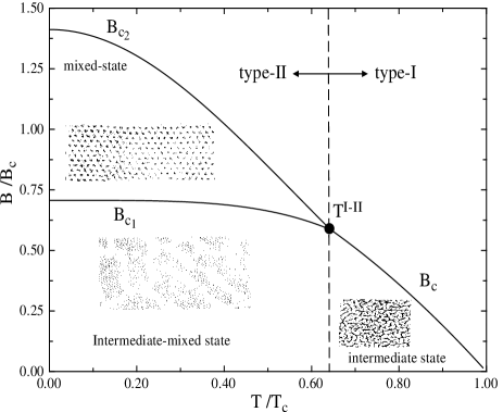
FIG. 1.: The thermodynamic phase diagram for a thin plate of a superconductor with $\kappa_{0}$ =1. The different transition lines corresponding to type-I and type-II superconducting behaviour meet in a multicritical point at a temperature $T^{I-II}$, where the order of the transition changes from first to second order. The phase lines are calculated from the two-fluid model (see text).

of type-I. Below $T^{I-II}$ however, the phase transition to the normal state happens at $B_{c_{2}}$ and thus the superconductor is of type-II. From the above arguments, we obtain for $T^{I-II}$

$$T^{I-II}=T_{c}(\sqrt{2}\kappa_{0}-1)^{1/2},$$ (5)

which only has a solution below $T_{c}$ for $1/\sqrt{2}<\kappa_{0}<\sqrt{2}$, putting a severe limit on the observability of the effect. More exact values may be determined from microscopic theories such as those of Helfand and Werthamer,taking the electron mean-free paths into account [5]. The results however do not differ greatly and would only be available numerically, thus obscuring the nature of the effects. In the B-T phase diagram, this point at which the fundamental behaviour of the superconductor changes may be interpreted as a multicritical point. An overview of this situation can be seen in Fig. 1, where we show the B-T phase diagram of a superconductor with $\kappa_{0}$ =1. The different transition lines $B_{c}$, $B_{c_{2}}$ and $B_{c_{1}}$ cross at the multicritical point at $T^{I-II}$. Furthermore, the phase transition at $B_{c}$ in a type-I superconductor is of first order, whereas that into a type-II superconductor at $B_{c_{2}}$ is of second order [4]. The third phase line $B_{c_{1}}$, separating the mixed state from the intermediate-mixed state in type-II superconductors depends on the value of $\kappa$ and the nature of the interactions between flux lines. For low $\kappa$ and attractive vortex interactions, the transition is thought to be of first order [6], otherwise it is second order. Thus we expect to observe a small region of coexistence between type-I and type-II superconducting behaviour around $T^{I-II}$. We will discuss this transition from type-I to type-II behaviour in more detail below in the discussion of the experimental findings.

II EXPERIMENT

We investigated four different samples of PbBi alloys, with different doping levels of Bi. For a typical example of type-I behaviour, we used a pure Pb sample and for a determination of the type-II properties we investigated a sample with a doping of 5$\%$ Bi. The samples with intermediate doping, 1.25 and 1.5$\%$, showed a transition from type-I to type-II behaviour at different fields and temperatures. The samples all were polycrystalline platelets of approximate dimensions 40x25x1 mm³, and an ellipsoidal cross-section. The samples were characterised with a vibrating sample magnetometer (VSM) and showed a superconducting transition, $T_{c}$ of 7.2 K in zero applied field.

The muon spin rotation ($\mu$SR) experiments were carried out at the MUSR instrument of the ISIS facility at the Rutherford Appleton Laboratory (RAL), UK. The ISIS facility provides a pulsed beam of positive muons at a frequency of 50 Hz with a pulse-width of $\simeq$ 70 ns. These muons are created in the decay of pions at rest and hence are almost fully spin polarised, antiparallel to their momentum, and have a kinetic energy of $\simeq$ 4 MeV. The neutron scattering measurements were done at the Institut Laue-Langevin (ILL), France, using the instrument D11. ILL provides the world’s most intense source of cold neutrons, where in our investigations we have used neutrons of a wavelength of 1.9 nm. For the very large structures in the intermediate mixed state, we needed to

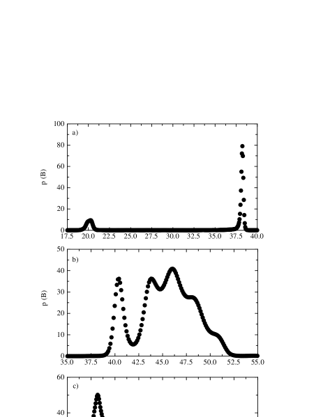
FIG. 2.: a) The local field distribution in the intermediate state. A background of muons stopping in the cryostat shows an applied field of 20 mT, while the muons in the sample precess at a frequency corresponding to 38 mT. This corresponds to the critical field $B_{c}$ at the temperature of 5.3 K, where the measurement was carried out. b) The local field distribution in the intermediate mixed state. The applied field can be seen to be 40 mT. In addition, there is a wide distribution of local fields corresponding to a vortex lattice at higher fields. The mean field of this flux lattice corresponds to the critical field at the transition from type-I to type-II behaviour $T^{I-II}$, if the overall field expulsion is taken into account (see text). The measurement was carried out at a temperature of 4.3 K. c) The field distribution for a vortex lattice, in the mixed state. The field distribution has a very characteristic shape, with a tail extending to fields higher than the average. The measurement was taken in an applied field of 30 mT in the type-II sample containing 5 $\%$ Bi.

observe small-angle scattering, for which D11 with a distance between the sample and the detector of up to 40 m is ideal. In the investigations described below, we have used a collimation length of 20.5 m and a sample-detector distance of 20 m. No beam stop was used. The neutrons are detected with a position-sensitive detector of 0.8x0.8 m² area and pixel size 10 mm. In both experiments, the field was applied at 45^∘ to the shortest direction of the sample, in order to have sizable demagnetisation fields.

In a transverse-field $\mu$SR experiment, positive muons come to rest in the bulk of a sample, where the field is applied perpendicular to the initial spin polarisation of the muons. Due to their magnetic moment, the muons then perform a Larmor-precession with a frequency proportional to the applied field. After a mean life-time of 2.2 $\mu$s, the muons decay into a positron (and two neutrinos). Due to parity violation in the weak decay of the muon, the decay-positron is preferentially emitted in the direction of the muon spin. Therefore the number of positrons observed at a fixed position, in the precession plane of the muons, will oscillate with time reflecting the Larmor-precession of the muons, in addition to an exponential decay, due to the radioactive decay of the muons. For a distribution of fields over the sample, as is the case for a vortex lattice, the oscillations due to the different fields superimpose giving rise to a depolarisation of the muons. In the case of large field gradients, the depolarisation rate may be fast enough to reduce the initial polarisation outside of the experimental time window. In the mixed state of a superconductor with short penetration depth, this may strongly reduce the signal observed by $\mu$SR. By studying the Fourier-transform of the number of decay positrons with time, we may however still observe the probability distribution of the internal fields, assuming a random distribution of muons over the sample. In order to avoid spurious noise in the Fourier-transform arising from the finite time window of observation, we use a maximum-entropy algorithm in our analysis [10]. This

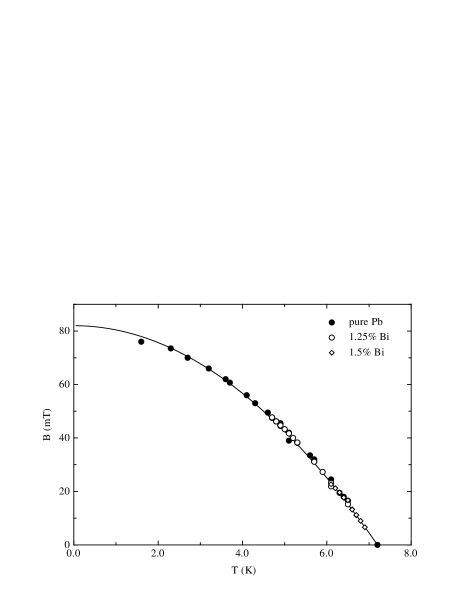
FIG. 3.: The thermodynamical critical field $B_{c}$, as determined from $\mu$SR in the intermediate state. The measurements are for all three samples exhibiting type-I behaviour. All curves were obtained with several applied fields, where the different determinations overlap (see text). It can also be seen that $B_{c}$ is the same for all samples in spite of the change in $\kappa$.

also prevents statistical noise at long times, due to low count rates, from spreading over the whole frequency domain. This is mainly because our algorithm never actually Fourier-transforms the raw data, but rather solves the inverse problem of calculating the frequency distribution and compares it to the time-data. A more detailed discussion can be found in Ref. [9].

For the vortex lattice, in the mixed state, the field distribution has a very specific shape, with a tail extending to fields higher than the average [11]. This is due to the high fields in the vortex cores. In the intermediate state, we expect a single-frequency signal at the critical field $B_{c}(T)$. The signal size in the intermediate state is given by the area fraction of the normal state domains. Neglecting the effects flux expulsion this is simply proportional to B / B_c(T), leading to a decrease in signal with decreasing temperature. Demagnetising effects due to the experimental geometry of having the field at 45^∘ to the plate however lead to a much stronger reduction of signal size with temperature. This leads to a dependence on the critical field $\propto 1/(B-B_{c})$, in reasonable agreement with the experimental findings. This may also be observed from the asymmetry in decay positrons upstream and downstream of the beamline. This corresponds to muons not precessing in a field that hence stopped in a Meissner domain in the sample. The temperature dependence of this signal is complementary to that observed from the normal state domains.

In a neutron scattering experiment, the neutrons are incident almost parallel to the applied field. The alignment of the beam with respect to the field was done by observing the diffraction pattern of the vortex lattice in a sample of Nb to an accuracy of 0.1^∘ both vertically and horizontally. Due to its magnetic moment, the neutron is scattered by gradients of magnetic field [3]. Therefore we may observe the domain pattern in the intermediate state in terms of a correlation function. In general, the scattered neutron intensity is given by [8]

$$I(Q)=\int R(Q)\frac{d\sigma(Q)}{d\Omega}dQ,$$ (6)

where Q is the scattering vector, $R(Q)$ is a resolution function, describing the distribution of neutrons around the nominal scattering vector $Q$. Finally, $d\sigma/d\Omega$ is given by [8]:

$$\frac{d\sigma(Q)}{d\Omega}\propto F(Q)S(Q),$$ (7)

where $F(Q)$ is a form factor describing the scattering of a basic building block of the structure and $S(Q)$ is a structure factor, describing the large scale structure. The fourier transform of the structure factor presents a measure of the ‘pair correlation’ or distance distribution function in the large scale structure. Thus eq. 7 corresponds to a convolution of the correlation functions of the two parts of the scattering.

In the intermediate state, this is a similar problem to that encountered in the study of vesicles of amphiphilic molecules that may build large scale structures. In contrast to these amphiphilic molecules however, the microscopic structure of the magnetic field domains is very simple. This microscopic structure is described by the London equations describing the magnetic behaviour of superconductors. Thus in the general expression for the scattered intensity, the form factor will be given by the well known London form factor. For the structure factor, we have used a model of randomly oriented chains with a radius of gyration R_g in the analysis of the measurements given below. This structure factor can be calculated to be [12]

$$S_{c}(Q)=\frac{2(exp(-R_{g}^{2}Q^{2})-1+R_{g}^{2}Q^{2})}{R_{g}^{4}Q^{4}}.$$ (8)

In the limit of large $R_{g}Q$, this form factor has the asymptotic dependence $S_{c}(Q)\propto Q^{-2}$, corresponding to a random walk arrangement of the chains. From the determination of $R_{g}$, we may then determine the contour length

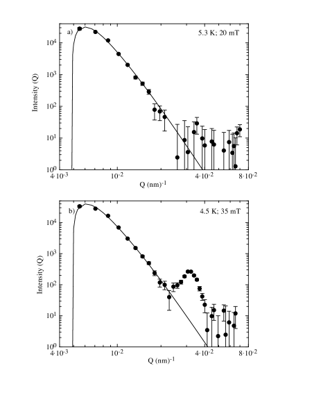
FIG. 4.: a) The scattered neutron intensity as a function of the scattering vector $Q$. A diffraction pattern above $T_{c}$ has been subtracted. The solid line presents a fit to a model using the structure factor of eq. 8. Thus we determine the radius of gyration and the interface area of the domain structure (see text). b) These measurements were done in the intermediate-mixed state. In addition to the structure factor from the domains in the intermediate-state, there is a strong peak corresponding to Bragg diffraction from the vortex lattice also present. The lattice spacing corresponds to a field of 45 mT, the critical field at $T^{I-II}$,the transition from type-I to type-II behaviour. The solid line represents a fit to the same model as above (see text).

of a chain, from $L=6R_{g}^{2}/b$, where we assume the statistical segment length $b$ to be the penetration depth. This model will break down below the length scale, where the magnetic domains become stiff. On this scale, a model of randomly distributed, solid rods is more appropriate. In this case, the structure factor has the asymptotic dependence $S_{r}\propto Q^{-1}$. For the magnetic domains, in the intermediate state, this length scale will be of the order of the penetration depth ($\lambda\simeq 90nm$). This makes it necessary to observe very small scattering vectors, in order to resolve the domain structure in the intermediate state. Due to the very small scattering angles the observed scattering distribution is also influenced by the width of the main beam. This may be taken into account by fitting a Gaussian distribution to the main beam in the normal state. The intensity of the main beam in the superconducting state is then reduced by those neutrons scattered according to $S_{c}(Q)$, whereas we assume the width of the main beam to be that in the normal state. From the radius of gyration thus determined we may then obtain the contour length of a domain in the intermediate state from

$$R_{g}^{2}=\frac{Lb}{6},$$ (9)

where the Kuhn segment $b$ is of the order of the penetration depth $\lambda$ and $L$ is the contour length. In Landau’s treatment of the intermediate state [13],the separation of the different domains in an equilibrium situation depends only on the thickness of the plate, the surface energy length $\delta$, usually associated with the coherence length in type-I superconductors and a universal function f(b), where b is the reduced field B/B_c. This function is calculated from the different energy scales of the order parameter and the magnetic field and is given by [13]

$$f(b)=\frac{1}{4\pi}[(1+b)^{4}ln(1+b)+(1-b)^{4}ln(1-b)$$ (10)

$$-(1+b^{2})^{2}ln(1+b^{2})-4b^{2}ln(8b)].$$

The separation of the different domains in the intermediate state is then given by the expression

$$L=\sqrt{\frac{d\delta}{f(b)}},$$ (11)

where $d$ is the thickness of the plate. In the case of interest here, where $\kappa$ is close to the boundary of 1/$\sqrt{2}$, the surface energy length becomes very small, such that the separation of the domains may of similar order as the separation of vortices in the mixed state and thus observable in neutron scattering experiments. This will be discussed further in the context of the experimental findings.

In the mixed state, the situation is simpler, as the scattering now is from a lattice. Therefore the structure factor will exhibit narrow peaks when the scattering vectors equal a reciprocal lattice vector. The big lattice spacing in the vortex lattice ($\sim$ 200 nm at 60 mT) leads to very small angles of scattering ($\sim 1^{\circ}$). In the intermediate-mixed state, there will be both structures, that of a vortex lattice and the characteristic domain structure of the intermediate state. The structure factor will thus be made up of a combination of both Bragg and domain-scattering.

III RESULTS AND DISCUSSION

A typical $\mu$SR measurement of the intermediate state in a type-I superconductor is shown in Fig. 2a) for the case of the 1.25 $\%$ Bi sample at a temperature of 5.3 K. Due to a small background of muons stopping in the cryostat, we observe the applied magnetic field (20 mT). There is also a second peak at the critical field $B_{c}$ corresponding to the temperature of 5.3 K. This field can be seen to be 38 mT in the figure. Thus we can map the phase boundary $B_{c}(T)$ in the type-I state, by measuring the local field in the sample at different temperatures. This is shown in Fig. 3 for the pure Pb sample, as well as the 1.25$\%$ Bi and 1.5$\%$ Bi samples in the type-I state. Due to the loss of signal with increasing field gradient, the measurements were performed over an overlapping range of applied fields. The observed $B_{c}(T)$ curve is found to be independent of the applied field. Furthermore, the temperature dependence of $B_{c}$ is in good agreement with the

FIG. 5.: The distribution of local fields as observed by $\mu$SR in the 1.25$\%$ Bi sample at a temperature of 4.7 K. The applied field is 40 mT. Moreover, one observes a sharp peak at a field corresponding to the critical field at that temperature (see Fig. 3). Finally one observes a very wide distribution of fields below $B_{c}$. This corresponds to flux lines that have nucleated out of the normalconducting regions in the intermediate state. Therefore in this situation, one observes a coexistence of the intermediate and the intermediate-mixed state, as would be expected at a multicritical point (see text).

expectations from the two-fluid model, as can be seen from the solid line in Fig. 3, representing a fit to eq. 2. Moreover, it can be seen in the figure that for the doped samples the value of $B_{c}$ remains unaltered. Considering the dependence of $B_{c}$ on the values of the coherence length and the penetration depth (eq. 1), we note that $\lambda^{\prime}\xi^{\prime}=\lambda\xi$, where $\lambda^{\prime}$ and $\xi^{\prime}$ are the values of the penetration depth and coherence length after doping. This agrees with the expectations of microscopic theories on the influence of impurities on the superconducting parameters in the temperature region of interest [5].

A typical SANS measurement of the intermediate state can be seen in Fig. 4a). This figure shows the 1.25$\%$ Bi sample at 5.3 K, as Fig. 2a) does for the $\mu$SR measurements. The intensity shown presents a subtraction of the scattering observed at 5.3 K and that above $T_{c}$. The data presents a radial average over the detector, giving the dependence of the scattered intensity on the absolute value of Q. The solid line in Fig. 4, represents a fit to eq. 7, where the structure factor was assumed to be given by eq. 8. Furthermore we have taken into account the effects arising from the very small scattering angles as discussed above. The value for the penetration depth used in calculating the London form factor was obtained from the $\mu$SR measurements on the vortex lattice in this sample. From this fit we determine the scattered intensity and the radius of gyration of the domain structure. Here, the scattered intensity presents a measure of the interface area between the domains and the radius of gyration roughly gives the size of the domains. This shows the very complementary results obtained from $\mu$SR and SANS.

Fig. 2b) shows the field probability distribution observed in $\mu$SR in the intermediate-mixed state. The measurement was done in the 1.25$\%$ Bi sample at a temperature of 4.3 K with an applied field of 40 mT. In addition to the background of muons stopping in the cryostat, we observe a signal arising from a flux line lattice with a mean field much higher than the applied. We will see below that the internal field corresponds to $B_{c}(T^{I-II})$, the critical field at the temperature where the superconducting behaviour changes. The same behaviour can be seen in Fig. 4b), where the scattered neutron intensity is shown at the same temperature, in an applied field of 35 mT. As in Fig.4a), the scattered intensity above $T_{c}$ has been subtracted and the London form factor has been taken into account. Similar to Fig. 4a), we observe scattering from the domain structure are low Q, that is similar to that observed in Fig. 4a), but in addition there is a peak in scattered intensity arising from the vortex lattice in the intermediate-mixed state. The plane spacing of this lattice, as obtained from the Q-value of the peak, corresponds to a mean field of a triangular lattice of 42 mT, in good agreement with the results from $\mu$SR. The plane spacing of the vortex lattice is connected to the field by the fact that each vortex line carries a quantum of flux. Thus the plane-spacing is given by $d=(\sqrt{3}/2\Phi_{0}/B)^{1/2}$ for a triangular lattice. From a comparison of Fig. 2b) with Fig. 2c), where the field distribution of a vortex lattice is shown, as obtained in the type-II sample containing 5 $\%$ Bi, it can be seen that the field distribution in the intermediate-mixed state does not perfectly match that of the mixed state. This may be understood from a comparison of the lattice spacing with the separation of the domains in the intermediate state. As will be shown below, they are of the same order of magnitude ($L\simeq 10\lambda$), which may lead to imperfections in the vortex lattice resulting in a more symmetric lineshape.

The value of the mean internal field in the intermediate-mixed state can be understood by considering the transition between type-I and type-II superconducting behaviour. The penetration of the field in the form of a vortex line arises from a competition between the surface energy gained by expelling the magnetic field to the cost of an inclusion of normalconducting material. The first will be roughly proportional to $\lambda$, whereas the second will be proportional to $\xi$ (see Ref.[7]). From this argument, it is seen that for a type-I superconductor, it is energetically unfavourable to build up domain boundaries. A rigorous calculation of these surface energies leads to the criterion of $\kappa=1/\sqrt{2}$ for the crossover from type-I to type-II behaviour when these energies are equal. We now consider the case of the intermediate-mixed state found in our samples at below $T^{I-II}$. On cooling the sample, it is in the intermediate state with normalconducting domains of mean field corresponding to $B_{c}(T)$. At the temperature $T^{I-II}$, the ratio of the surface energies passes through one. Thus as discussed above the formation of normalconducting-superconducting boundaries becomes energetically favourable. This corresponds to a sign-change of an effective surface tension of the magnetic field in the domains, leading to the nucleation of vortices from the normalconducting domains, due to flux quantisation in the superconductor. The domain structure however, remains the same, which is why the mean field of the vortex lattice corresponds to the value of $B_{c}(T^{I-II})$, due to flux conservation.

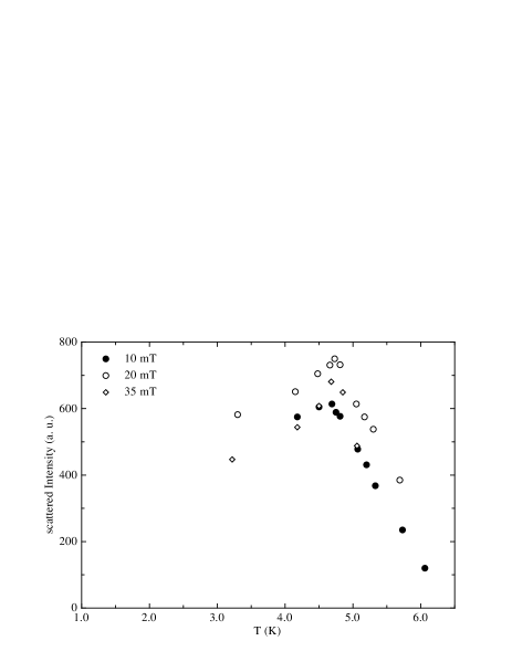
FIG. 6.: The scattered neutron intensity from the domain structure in the intermediate and intermediate-mixed state as a function of temperature at three different applied fields in the 1.25$\%$ Bi sample. The scattered intensity was obtained by a fit using the model given by eq. 8. This presents a measure of the interface area of the domains, thus describing the ruggedness of the flux distribution in the sample (see text). As would be expected the scattered intensity shows a maximum around the temperature $T^{I-II}$, where vortices are nucleating from the normal domains (see text).

As the order of the superconducting transition changes between a type-I and type-II superconductor in a magnetic field, the point in the B-T phase diagram at $T^{I-II}$ may also be interpreted as a multicritical point. In this scenario, we would expect to see a co-existence of the intermediate and the intermediate-mixed state over a short temperature interval. That this is in fact the case can be seen in Fig. 5, where we show the local field distribution observed from $\mu$SR at a temperature of 4.7 K in the 1.25$\%$ Bi sample. As can be seen in the figure, in addition to the sharp peaks at the applied field and $B_{c}$, there is a field distribution at fields just below $B_{c}$. This coexistence of the intermediate and the intermediate-mixed state is observed over a temperature interval of 0.4 K. Within our temperature resolution of 0.1 K there is no hysteresis observable in the ratio between the two states.

From the onset of superconducting behaviour at higher fields, we determine the value of $B_{c_{2}}$, which together with the value of $B_{c}$ determined from the Pb sample results in a determination of $\kappa_{0}$. For the two samples showing a transition from type-I to type-II behaviour, this results in $\kappa_{0}^{1.25}$ = 1.02(2) and $\kappa_{0}^{1.5}$ = 1.21(3). Using eq. 5, we may then estimate the transition temperature $T^{I-II}$, resulting in $T^{I-II}_{1.25}$ = 4.8(2) K and $T^{I-II}_{1.5}$ = 6.1(1) K. These values are in excellent agreement with those obtained directly in both $\mu$SR and SANS from the appearance of the intermediate-mixed state. These directly determined values are $T^{I-II}_{1.25}$ = 4.7(1) K and $T^{I-II}_{1.5}$ = 6.2(1) K. This also indicates that the phenomenological two-fluid model gives a fair description of the superconducting behaviour of these PbBi alloys.

We now briefly return to the observation of the intermediate state with SANS. As already noted above, from the structure factor we determined in the intermediate state, we may obtain a measure of the interface area from the total scattered intensity, as well as the radius of gyration of the domain structure. Both these quantities depend upon temperature. At high temperatures, close to $T_{c}$, the critical field is close to the applied field, such that most of the sample area will be in the normal state and the domain interface will be small. At low temperatures, the critical field is much higher than the applied field and only a very small area will be in the normal state. Thus again the domain interface will be small. Therefore the scattered intensity will exhibit a maximum with temperature, where the domain structure is most convolved. This can be seen in Fig 6, where we show the temperature dependence of the scattered intensity in the 1.25$\%$ Bi sample at different applied fields. As can be seen in the figure, the intensity shows a marked peak at the transition temperature $T^{I-II}$ and then decreases slowly at low temperatures. Such a sharp peak in the region of coexistence between the intermediate and the intermediate-mixed state is possibly due to the strong increase in surface area of the magnetic flux structures when the two states coexist. At this point, the domain structure does not change, but the normalconducting regions are nucleating vortex lines, leading to both an enhancement in the surface area and the size of the magnetic domain structures. The width of the coexistence is similar to that found by $\mu$SR. The decrease in intensity is faster at higher applied fields. This may arise from the fact that these high fields are already sufficiently close to $B_{c_{1}}$, such that the superconductor would simply be in the mixed state at low temperature. Hence there would be no scattering from domains in that situation.

In the same way, we may investigate the size of the domains from the radius of gyration observed in the intermediate state. Using the relationships between the radius of gyration determined from the fits to the scattered neutron intensities with the separation of the domains and Landau’s expression for this separation, we may also determine the universal function f(b). With the known thickness of the sample of 1 mm, there are two adjustable parameters left, whose order of magnitude is known. These are the Kuhn length of the segments of the chains that is roughly given by the penetration depth and the surface energy length that has to be somewhat smaller than the coherence length. Using a segment length equal to the penetration depth, the surface energy length $\delta$ = 10 nm has to be chosen to obtain reasonable agreement with the expectations from Landau

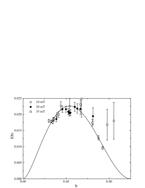
FIG. 7.: The function f(h) from Landau theory, as determined from the radius of gyration of the normalconducting domains in the intermediate and the intermediate-mixed state. The temperature dependences at different fields allow us to determine f(h) over a big range of reduced fields. In order to obtain reasonable agreement of the size of the domains with the predictions of Landau theory, a surface energy length of 10 nm, much smaller than the coherence length had to be assumed. This is however not unreasonable, given the closeness of $\kappa$ to 1/$\sqrt{2}$ (see text).

theory for f(b). These results can be seen in Fig. 7 for the 1.25 $\%$ sample. The use of the temperature dependences at the different fields results in a determination of f(b) over a big range of values. The value of $\delta$ used to obtain the agreement with Landau theory is an order of magnitude smaller than the coherence length. This is however not unexpected, as the value of $\kappa$ is very close to its boundary value of 1/$\sqrt{2}$ and hence the surface energy length is expected to be small as discussed above.

IV CONCLUSIONS

We have measured the behaviour of type-I and type-II superconductors in a magnetic field. It is shown that there is a transition from type-I to type-II behaviour with temperature. This transition happens at a temperature well defined in the framework of the two-fluid model and can be shown to only arise for superconductors with a Ginzburg-Landau parameter in the interval $1/\sqrt{2}<\kappa_{0}<\sqrt{2}$ at low temperature. This transition may be seen as a multicritical point in the B-T phase diagram of superconductors, as the order of the superconducting transition is changed from first to second order. Therefore we also observe a coexistence of the different behaviours around the transition with both SANS and $\mu$SR. We furthermore use the complementarities of SANS and $\mu$SR to study the intermediate state in type-I superconductors. Using SANS, we observe the domain structure via the interface area given by the scattered intensity and the domain sizes via the radius of gyration, where there is qualitative agreement with the treatment of the intermediate state by Landau. The local fields are investigated with $\mu$SR, where we can map the critical field as a function of temperature.

V Acknowledgements

We would like to thank the staff at ILL (Andreas Polzak) and ISIS (Chris Scott, James Lord) for technical assistance, as well as the Swiss National Science Foundation and the EPSRC of the UK for financial support.

REFERENCES

- [1] Present address: Vrije Universiteit Amsterdam, De Boelelaan 1081, 1081HV Amsterdam, The Netherlands.
- [2] M. Tinkham,Introduction to Superconductivity, 3rd Edition McGraw-Hill, New York (1996).
- [3] D. Cribier, B. Jacrot, L. Madhov Rao, B. Farnoux, Phys. Lett. 9, 106 (1964).
- [4] D. R. Tilley and J. Tilley, Superfluidity and Superconductivity, 3rd Edition, IOP publishing, 1990.
- [5] E. Helfand and N. R. Werthamer, Phys. Rev. Lett. 13, 686 (1964); Phys.Rev. 147, 288 (1966).
- [6] J. Auer and H. Ullmaier, Phys. Rev. B 7, 136 (1973).
- [7] K. Kopitzki, Einführung in die Festkörperphysik, B.G.Teubner (Stuttgart), 1993.
- [8] G. L. Squires, Introduction to the Theory of Thermal Neutron Scattering, Cambridge University Press, 1978.
- [9] C. M. Aegerter, J. Hofer, I. M. Savić, H. Keller, S. L. Lee, C. Ager, S. H. Lloyd, E. M. Forgan, Phys. Rev. B 57, 1253 (1998).
- [10] B. D. Rainford, G. J. Daniell, Hyperfine Interactions 87, 1129 (1994).
- [11] A. D. Sidorenko, V. P. Smilga, V. I. Fresenko, Hyperfine Interactions 63, 49 (1990).
- [12] P. Debye J. Phys. Colloid Chem. 51, 18 (1947); J. S. Pedersen and M. C. Gerstenberg, Macromolecules 29, 1363 (1996).
- [13] L. D. Landau and E. M. Lifshitz, Electrodynamics of Continuous Media, Pergamon Press, New York (1984); L. D. Landau, JETP 7, 371 (1937).