Collective excitations in trapped boson-fermion mixtures: from demixing to collapse

Abstract

We calculate the spectrum of low-lying collective excitations in a gaseous cloud formed by a Bose-Einstein condensate and a spin-polarized Fermi gas over a range of the boson-fermion coupling strength extending from strongly repulsive to strongly attractive. Increasing boson-fermion repulsions drive the system towards spatial separation of its components (“demixing”), whereas boson-fermion attractions drive it towards implosion (“collapse”). The dynamics of the system is treated in the experimentally relevant collisionless regime by means of a Random-Phase approximation and the behavior of a mesoscopic cloud under isotropic harmonic confinement is contrasted with that of a macroscopic mixture at given average particle densities. In the latter case the locations of both the demixing and the collapse phase transitions are sharply defined by the same stability condition, which is determined by the softening of an eigenmode of either fermionic or bosonic origin. In contrast, the transitions to either demixing or collapse in a mesoscopic cloud at fixed confinement and particle numbers are spread out over a range of boson-fermion coupling strength, and some initial decrease of the frequencies of a set of collective modes is followed by hardening as evidenced by blue shifts of most eigenmodes. The spectral hardening can serve as a signal of the impending transition and is most evident when the number of bosons in the cloud is relatively large. We propose physical interpretations for these dynamical behaviors with the help of suitably defined partial compressibilities for the gaseous cloud under confinement.

I Introduction

Dilute boson-fermion mixtures are currently being produced and studied in several experiments by trapping and cooling vapors of mixed alkali-atom isotopes Schreck et al. (2001); Goldwin et al. (2002); Hadzibabic et al. (2002); Roati et al. (2002); Modugno et al. (2002); Ferlaino et al. (2003). The large variety of combinations of atomic species and of choices of magnetic sublevels, together with the additional possibility of tuning the interactions by means of Feshbach resonances provide a unique opportunity of investigating extensively the effects of boson-fermion interactions, both in the case of mutual repulsions and in the case of attractions.

The boson-fermion coupling strongly affects the equilibrium properties of the mixture and can lead to quantum phase transitions. Boson-fermion repulsions can induce spatial demixing of the two components when the interaction energy overcomes the kinetic and confinement energies Mølmer (1998), and several configurations with different topology are possible for a demixed cloud inside a harmonic trap Akdeniz et al. (2002a). Although spatial demixing has not yet been experimentally observed, the ⁶Li-⁷Li experiments of Schreck et al. Schreck et al. (2001) appear to be quite close to the onset of the demixed state Akdeniz et al. (2002b). In the case of attractive boson-fermion coupling the mixture becomes unstable against collapse when the boson-induced fermion-fermion attractions overcome the Pauli pressure Mølmer (1998); Miyakawa et al. (2001). Collapse has been experimentally observed in a ⁴⁰K-⁸⁷Rb mixture Modugno et al. (2002). Fermion pairing into a superfluid state has also been predicted in the case of attractive interactions Efremov and Viverit (2002), but for spin-polarized fermions this is expected to happen in the $p$-wave channel at temperatures much lower than the current experimental limit. This possibility will not be considered in the present work.

The dynamical properties of boson-fermion mixtures have been previously investigated theoretically mainly in the mixed phase, both for the macroscopic homogeneous system Yip (2001); Search et al. (2002); Viverit and Giorgini (2002) and in mesoscopic clouds inside a harmonic trap. In the latter case these studies have used a sum-rule approach Miyakawa et al. (2000); Liu and Hu (2003), perturbation theory Minguzzi and Tosi (2000), or a Random-Phase approximation (RPA) Capuzzi and Hernández (2001); Sogo et al. (2002); Capuzzi and Hernández (2002).

In this paper we investigate the effect of boson-fermion interactions on the spectrum of collective excitations as the mixture approaches an instability and look for the dynamical signatures of the approaching instabilities. In a previous paper Capuzzi et al. (2003) we have studied the transition to demixing of a confined cloud in the collisional regime and found an analytical condition for the dynamical transition point. We focus here on the experimentally more relevant case of the collisionless regime, where we adopt an RPA scheme. Within this formalism it is possible to study at the same level the evolution of the cloud towards demixing on one side and collapse on the other, thus providing a unified picture of very different states. We characterize the dynamical properties of the mixture not only by its spectrum but also through its generalized partial compressibilities.

We comparatively examine a homogeneous mixture and a mixture in external harmonic confinement. Whereas in the former case the RPA spectra are symmetric under changing the sign of the boson-fermion coupling, inside the trap we find different behaviors on going from the case of boson-fermion repulsions to that of attractions. This is due to the fact that in the theory the transition in the macroscopic homogeneous system is approached at fixed density of the two species, while in the trapped mesoscopic cloud we work in the realistic situation of constant particle numbers and fixed external confinement.

The paper is organized as follows. In Sec. II we review the conditions for demixing and collapse as obtained from static considerations, and in Sec. III we introduce the RPA formalism for the collective excitation spectrum. Sec. IV describes the predictions of the RPA for the case of a homogeneous system, while Sec. V reports the results for the collective excitation spectrum of a mixture under external harmonic confinement. Finally, Sec. VI contains a summary and our main conclusions.

II Equilibrium state: conditions for demixing and collapse

We consider a dilute boson-fermion mixture at zero temperature. The Hamiltonian which describes the system is

$$H = \sum_{\sigma=B,F}\int d^{3}r\,\Psi^{\dagger}_{\sigma}\left(-\frac{\hbar^{2}\nabla^{2}}{2m_{\sigma}}+V_{ext}^{\sigma}({\mathbf{r}})-\mu_{\sigma}\right)\Psi_{\sigma}$$ (1)

$$+ \frac{g_{BB}}{2}\int d^{3}r\,\Psi^{\dagger}_{B}\Psi^{\dagger}_{B}\Psi_{B}\Psi_{B}+g_{BF}\int d^{3}r\,\Psi^{\dagger}_{B}\Psi^{\dagger}_{F}\Psi_{F}\Psi_{B}$$

where $\Psi_{B}$ and $\Psi_{F}$ are the usual bosonic and fermionic field operators, $V_{ext}^{B,F}({\mathbf{r}})$ are the external confining potentials, $\mu_{B,F}$ are the chemical potentials, and $m_{B,F}$ the atomic masses. We have introduced the couplings $g_{BB}=4\pi\hbar^{2}a_{BB}/m_{B}$ for boson-boson interactions and $g_{BF}=2\pi\hbar^{2}a_{BF}/m_{r}$ for boson-fermion interactions, in terms of the $s$-wave scattering lengths $a_{BB}$ and $a_{BF}$ and of the reduced boson-fermion mass $m_{r}$. We will always assume $a_{BB}>0$. We are here neglecting the fermion-fermion interactions since we are considering a spin-polarized Fermi gas where $s$-wave collisions are forbidden by the Pauli principle and higher-order collisional couplings are negligible at the temperatures of present interest. In the dilute limit we also neglect the quantum depletion of the condensate.

The equilibrium state of the mixture is described at mean field level by the self-consistent solution of the Gross-Pitaevskii equation for the condensate extended to include the boson-fermion interactions,

$$\left[-\frac{\hbar^{2}\nabla^{2}}{2m_{B}}+V_{ext}^{B}({\mathbf{r}})+g_{BB}\,n_{B}({\mathbf{r}})+g_{BF}\,n_{F}({\mathbf{r}})\right]\Phi_{B}({\mathbf{r}})=\mu_{B}\Phi_{B}({\mathbf{r}})$$ (2)

and by the Hartree-Fock equations for the fermions coupled to the boson density,

$$\left[-\frac{\hbar^{2}\nabla^{2}}{2m_{F}}+V_{ext}^{F}({\mathbf{r}})+g_{BF\,}n_{B}({\mathbf{r}})\right]\psi_{i}({\mathbf{r}})=\varepsilon_{i}\psi_{i}({\mathbf{r}}).$$ (3)

In Eqs. (2) and (3) the condensate density is given by

$$n_{B}({\mathbf{r}})=|\Phi_{B}({\mathbf{r}})|^{2}$$ (4)

and the fermion density by

$$n_{F}({\mathbf{r}})=\sum_{i}|\psi_{i}({\mathbf{r}})|^{2}\,\theta(\mu_{F}-\varepsilon_{i}).$$ (5)

The chemical potentials are obtained by imposing the normalization conditions $N_{B,F}=\int d^{3}r\,n_{B,F}({\mathbf{r}})$ giving the numbers of particles of the two species. Excited-state condensate wave functions and Hartree-Fock orbitals will also be needed in the construction of the RPA dynamical susceptibilities in Sec. III.

Under isotropic harmonic confinement $V_{ext}^{B,F}(\mathbf{r})=m_{B,F}\omega_{B,F}^{2}r^{2}/2$, for the values of $N_{F}\sim 10^{4}$ as in current experiments we have verified that the fermionic equilibrium profiles are well described by the solution of the generalized Thomas-Fermi approximation (TFA)

$$-\frac{\hbar^{2}}{6m_{F}}\frac{\nabla^{2}\sqrt{n_{F}({\mathbf{r}})}}{\sqrt{n_{F}({\mathbf{r}})}}+An_{F}^{2/3}({\mathbf{r}})+V_{ext}^{F}({\mathbf{r}})+g_{BF\,}n_{B}({\mathbf{r}})=\mu_{F},$$ (6)

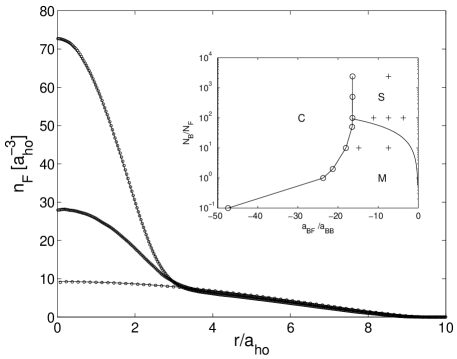
Figure 1: Equilibrium density profiles $n_{F}(r)$ (in units of $a_{ho}^{-3}$) as functions of the radial coordinate $r$ (in units of $a_{ho}$) for the fermionic component of a ⁶Li-⁷Li mixture under isotropic harmonic confinement, as obtained from the solution of the Hartree-Fock equations (dots) and from the Thomas-Fermi approximation (solid line, hidden by the dots). The curves from top to bottom correspond to the choices $a_{BF}=-4$ nm, $a_{BF}=-2$ nm, and $a_{BF}=0$. The other parameters are $N_{B}=10^{5}$, $N_{F}=10^{4}$, $a_{BB}=0.27$ nm and $\omega_{0}=2\pi\times 1000$ sec^-1. The inset reports the phase diagram of the mixture with boson-fermion attractions in the adimensional variables $a_{BF}/a_{BB}$ (linear scale) and $N_{B}/N_{F}$ (log scale), showing the regions of stability (S), metastability (M) and collapse (C). The crosses show the points where the spectra of the trapped mixture are explored in this paper.

which includes the surface kinetic energy effects in the form of von Weiszäcker Capuzzi et al. (2003). Here $A=(\hbar^{2}/2m_{F})(6\pi^{2})^{2/3}$. The fermionic density profiles for various values of the boson-fermion coupling $g_{BF}<0$ are shown in Fig. 1. The result of the TFA is practically indistinguishable from the full solution of Eqs. (3) and (5), since the shell effects play only a marginal role in the spherically symmetric case for the above choice of fermion number. The inset in Fig. 1 reports the phase diagram of the harmonically confined mixture for the case $g_{BF}<0$ (see below).

At increasing values of the boson-fermion coupling the mixture becomes unstable against demixing (in the case $g_{BF}>0$) or collapse (in the case $g_{BF}<0$) Mølmer (1998). In a homogeneous system at fixed particle densities a linear stability analysis based on a mean-field energy functional predicts the same condition for collapse and for demixing Viverit et al. (2000):

$$g_{BB}g_{FF}-g_{BF}^{2}=0$$ (7)

with $g_{FF}=(2/3)An_{F}^{-1/3}$ playing the role of an effective fermion-fermion coupling due to the Pauli pressure in the Fermi gas.

In the presence of external harmonic confinement the effects of finiteness substantially modify the description of the instabilities. In the case of demixing the transition is smoothed out and the onset of demixing with increasing boson-fermion coupling is signalled first by a diminishing boson-fermion overlap energy Akdeniz et al. (2002a). The condition of such partial demixing is given by

$$\frac{g_{BF}^{part}}{g_{BB}}=\left(c_{1}\,\frac{N_{F}^{1/2}}{N_{B}^{2/5}}+c_{2}\,\frac{N_{B}^{2/5}}{N_{F}^{1/3}}\right)^{-1},$$ (8)

where the parameters are $c_{1}=(15^{3/5}/48^{1/2})(m_{F}/m_{B})^{3/2}(a_{BB}/a_{ho})^{3/5}$ and $c_{2}=(48^{1/3}/15^{3/5})(6/\pi)^{2/3}(a_{BB}/a_{ho})^{2/5}$, with $a_{ho}=(\hbar/m_{B}\omega_{B})^{1/2}$. On further increase of the boson-fermion coupling one reaches the point where the fermionic density vanishes at the center of the trap, which occurs at

$$\frac{g_{BF}^{dyn}}{g_{BB}}=\frac{\mu_{F}}{\mu_{B}}.$$ (9)

This condition also corresponds to a sharp upturn in the frequencies of collective excitations in the collisional regime Capuzzi et al. (2003). If the boson-fermion coupling is further increased the overlap between the two clouds becomes negligible, the point of full spatial separation being well predicted by Eq. (7) in a local-density approximation Akdeniz et al. (2002b). At full separation the most likely configuration with current experimental parameters e.g.  in a ⁶Li-⁷Li mixture Schreck et al. (2001) is the “egg” configuration, formed by a core of bosons surrounded by a shell of fermions.

In the case of attractive interactions, at increasing values of the boson-fermion coupling the cloud is predicted to enter first a region of metastability where the zero-point oscillations still prevent collapse. For equal masses and trapping frequencies the condition of metastability as derived by Miyakawa et al. Miyakawa et al. (2001) is given by

$$\frac{|g_{BF}^{meta}|}{g_{BB}}\geq\frac{N_{B}}{2^{5/2}\,N_{F}}.$$ (10)

On further increase of $|g_{BF}|$ the mixture reaches the point of collapse, that in the numerical solution of the equilibrium equations (2) and (6) we localize at the point where convergence fails. We have verified that this instability point is well described by Eq. (7) in a local-density approximation Mølmer (1998); Miyakawa et al. (2001),

$$\frac{|g_{BF}^{coll}|}{g_{BB}}=\left[\frac{\pi m_{B}}{2m_{F}}\frac{1}{(6\pi^{2}n_{F}(0))^{1/3}a_{BB}}\right]^{1/2}$$ (11)

where $n_{F}(0)$ is the fermion density at the center of the trap. From the conditions (10) and (11) it can be seen that for large boson numbers $N_{B}\gg N_{F}$ the metastability region is absent and the cloud is predicted to go directly from a stable to an unstable configuration. The inset in Fig. 1 shows the phase diagram of the confined mixture in the case $g_{BF}<0$ with the choice of parameters that we shall adopt later in the study of the RPA spectrum of collective excitations. Similar curves for the critical boson number needed to reach collapse have been reported by Roth Roth (2002).

In summary, the criterion obtained in Eq. (7) for a macroscopic cloud is still useful to locate within a local-density approximation the end of the transition to either demixing or collapse in a boson-fermion mixture inside a harmonic trap. However, the transitions in a mesoscopic cloud kept under fixed external confinement are spread out and their approach will best be characterized by dynamical signatures, as we proceed to show below by spectral calculations in cases of increasing boson-fermion coupling.

III The Random-Phase approximation for a boson-fermion mixture

The RPA is equivalent to a time-dependent Hartree-Fock theory of the dynamics of a quantum fluid in the collisionless regime Pines and Nozières (1966) and was first introduced for dilute boson-fermion mixtures under confinement by Capuzzi and Hernández Capuzzi and Hernández (2001). It treats on the same footing the density fluctuations of the two atomic species, satisfying the f-sum rules and allowing for Landau damping of the bosonic excitations by the Fermi cloud. Since it neglects correlations between density fluctuations, the RPA is valid in the dilute limit specified by the inequalities $n_{B}a_{BB}^{3}\ll 1$ and $k_{F}|a_{BF}|\ll 1$, where $k_{F}=(6\pi^{2}n_{F})^{1/3}$ is the Fermi wave number.

The RPA yields the spectrum of collective excitations in the linear regime from a set of coupled equations for the density fluctuations $\delta n_{F}$ and $\delta n_{B}$, which are obtained by assuming that the fluid responds as an ideal gas to external perturbing fields $\delta U_{F}$ and $\delta U_{B}$ plus the Hartree-Fock fluctuations. The RPA equations in Fourier transform with respect to the time variable read

$$\delta n_{F}({\mathbf{r}},\omega)=\int d^{3}r^{\prime}\,\chi^{0F}({\mathbf{r}},{\mathbf{r}^{\prime}},\omega)[\delta U_{F}({\mathbf{r}^{\prime}},\omega)+g_{BF}\,\delta n_{B}({\mathbf{r}^{\prime}},\omega)]$$ (12)

and

$$\delta n_{B}({\mathbf{r}},\omega)=\int d^{3}r^{\prime}\,\chi^{0B}({\mathbf{r}},{\mathbf{r}^{\prime}},\omega)[\delta U_{B}({\mathbf{r}^{\prime}},\omega)+g_{BB}\,\delta n_{B}({\mathbf{r}^{\prime}},\omega)+g_{BF}\,\delta n_{F}({\mathbf{r}^{\prime}},\omega)].$$ (13)

In the inhomogeneous system consistency between equilibrium and dynamics requires to take into account static mean-field interactions. Thus $\chi^{0F}$ in Eq. (12) is the Lindhard density-density response function constructed with the Hartree-Fock orbitals from Eq. (3),

$$\chi^{0F}({\mathbf{r}},{\mathbf{r}^{\prime}},\omega)=\sum_{i,j}\frac{f(\varepsilon_{i})-f(\varepsilon_{j})}{\omega-(\varepsilon_{j}-\varepsilon_{i})+i\eta}\psi_{i}({\mathbf{r}})\psi^{*}_{i}({\mathbf{r}^{\prime}})\psi_{j}({\mathbf{r}^{\prime}})\psi^{*}_{j}({\mathbf{r}})$$ (14)

with $f(\varepsilon)=\theta(\mu_{F}-\varepsilon)$ and $\eta=0^{+}$. Similarly, $\chi^{0B}$ in Eq. (13) is the condensate density-density response function constructed with the excited states $\phi_{i}$ of the Gross-Pitaevskii equation with energy eigenvalues $E_{i}$,

$$\chi^{0B}({\mathbf{r}},{\mathbf{r}^{\prime}},\omega)=\sum_{i\neq 0}\left[\frac{\Phi_{B}({\mathbf{r}})\Phi_{B}^{*}({\mathbf{r}^{\prime}})\phi_{i}^{*}({\mathbf{r}^{\prime}})\phi_{i}({\mathbf{r}})}{\omega-(E_{i}-\mu_{B})+i\eta}-\frac{\Phi_{B}({\mathbf{r}^{\prime}})\Phi_{B}^{*}({\mathbf{r}})\phi_{i}^{*}({\mathbf{r}})\phi_{i}({\mathbf{r}^{\prime}})}{\omega+(E_{i}-\mu_{B})+i\eta}\right].$$ (15)

The RPA Eqs. (12) and (13) are most easily solved in terms of a matrix of density-density response functions, which are defined as

$$\chi_{\sigma\sigma^{\prime}}({\mathbf{r}},{\mathbf{r}^{\prime}},t-t^{\prime})=\frac{\delta n_{\sigma}({\mathbf{r}},t)}{\delta U_{\sigma^{\prime}}({\mathbf{r}^{\prime}},t^{\prime})}=-i\theta(t-t^{\prime})\langle[\delta\rho_{\sigma}({\mathbf{r}},t),\delta\rho_{\sigma^{\prime}}({\mathbf{r}^{\prime}},t^{\prime})]\rangle,$$ (16)

where $\delta\rho_{\sigma}(\mathbf{r},t)$ are the density fluctuations operators in the Heisenberg representation. Upon introducing the matrices $\bar{\chi}=\left(\begin{array}[]{cc}\chi_{FF}&\chi_{FB}\\ \chi_{BF}&\chi_{BB}\end{array}\right)$, $\bar{\chi}^{0}=\left(\begin{array}[]{cc}\chi^{0F}&0\\ 0&\chi^{0B}\end{array}\right)$, and $G=\left(\begin{array}[]{cc}0&g_{BF}\\ g_{BF}&g_{BB}\end{array}\right)$ the RPA equations read

$$\bar{\chi}({\mathbf{r}},{\mathbf{r}^{\prime}},\omega)=\bar{\chi}^{0}({\mathbf{r}},{\mathbf{r}^{\prime}},\omega)+\int d^{3}r^{\prime\prime}\,\bar{\chi}^{0}({\mathbf{r}},{\mathbf{r}^{\prime\prime}},\omega)\,G\,\bar{\chi}({\mathbf{r}^{\prime\prime}},{\mathbf{r}^{\prime}},\omega).$$ (17)

In fact, the boson-boson interactions can be resummed into the Bogoliubov response functions $\chi^{Bog}$, defined from

$$\chi^{Bog}({\mathbf{r}},{\mathbf{r}^{\prime}},\omega)=\chi^{0B}({\mathbf{r}},{\mathbf{r}^{\prime}},\omega)+\int d^{3}r^{\prime\prime}\,\chi^{0B}({\mathbf{r}},{\mathbf{r}^{\prime\prime}},\omega)\,g_{BB}\,\chi^{Bog}({\mathbf{r}^{\prime\prime}},{\mathbf{r}^{\prime}},\omega).$$ (18)

Thus the RPA equation can alternatively be expressed as

$$\bar{\chi}({\mathbf{r}},{\mathbf{r}^{\prime}},\omega)=\tilde{\chi}^{0}({\mathbf{r}},{\mathbf{r}^{\prime}},\omega)+\int d^{3}r^{\prime\prime}\,\tilde{\chi}^{0}({\mathbf{r}},{\mathbf{r}^{\prime\prime}},\omega)\,\tilde{G}\,\bar{\chi}({\mathbf{r}^{\prime\prime}},{\mathbf{r}^{\prime}},\omega)$$ (19)

with $\tilde{\chi}^{0}=\left(\begin{array}[]{cc}\chi^{0F}&0\\ 0&\chi^{Bog}\end{array}\right)$ and $\tilde{G}=\left(\begin{array}[]{cc}0&g_{BF}\\ g_{BF}&0\end{array}\right)$. In this way the excitations of the bosonic cloud are described as a gas of Bogoliubov phonons interacting only with the fermions.

IV Spectra of the homogeneous mixture

The RPA equations for the homogeneous fluid mixture with average particle densities $n_{B}$ and $n_{F}$ can be solved algebraically in Fourier transform with respect to the relative position coordinate $\mathbf{r}-\mathbf{r}^{\prime}$. The solution takes the form

$$\bar{\chi}({\mathbf{k}},\omega)=\frac{1}{\epsilon({\mathbf{k}},\omega)}\left(\begin{array}[]{cc}\chi^{0F}({\mathbf{k}},\omega)&g_{BF}\,\chi^{Bog}({\mathbf{k}},\omega)\,\chi^{0F}({\mathbf{k}},\omega)\\ g_{BF}\,\chi^{Bog}({\mathbf{k}},\omega)\,\chi^{0F}({\mathbf{k}},\omega)&\chi^{Bog}({\mathbf{k}},\omega)\end{array}\right)$$ (20)

where the “dielectric function” $\epsilon({\mathbf{k}},\omega)$ is the common denominator of the four partial responses and is given by

$$\epsilon({\mathbf{k}},\omega)=1-g_{BF}^{2}\,\chi^{Bog}({\mathbf{k}},\omega)\,\chi^{0F}({\mathbf{k}},\omega).$$ (21)

The spectrum of collective excitations is obtained by searching for the poles of the response matrix or equivalently by imposing $\epsilon({\mathbf{k}},\omega)=0$ in the complex frequency plane. In Eqs. (20) and (21) the Bogoliubov response function is

$$\chi^{Bog}({\mathbf{k}},\omega)=\frac{n_{B}^{2}k^{2}/m_{B}}{\omega\,(\omega+i\eta)-c_{B}^{2}k^{2}-(\hbar k^{2}/2m_{B})^{2}}$$ (22)

with $c_{B}=(g_{BB}n_{B}/m_{B})^{1/2}$, and the Lindhard response function is

$$\chi^{0F}({\mathbf{k}},\omega)=\sum_{\mathbf{p}}\frac{f(\varepsilon_{{\mathbf{p}}})-f(\varepsilon_{{\mathbf{p}}+{\mathbf{k}}})}{\omega-(\varepsilon_{{\mathbf{p}}+{\mathbf{k}}}-\varepsilon_{{\mathbf{p}}})+i\eta}$$ (23)

where $\varepsilon_{\mathbf{k}}=\hbar k^{2}/2m_{F}$. The summation in Eq. (23) can be carried out explicitly (see e.g. the book of Fetter and Walecka Fetter and Walecka (1971)) to yield the spectrum of single particle-hole pair excitations and the corresponding reversible part of the susceptibility of the ideal Fermi gas.

Equations (20) and (21) were first introduced by Yip Yip (2001), who evaluated numerically the spectra in the case of weak boson-fermion coupling. For $c_{B}>v_{F}$, where $v_{F}=\hbar k_{F}/m_{F}$ is the Fermi velocity, the spectrum at $g_{BF}=0$ contains a stable bosonic phonon and a fermionic particle-hole continuum. When the boson-fermion interactions are turned on these modes hybridize and repel each other, as can be analytically shown in the long wavelength limit. From the condition $\epsilon({\mathbf{k}},\omega)=0$, using Eq. (22) and $\chi^{0F}({\mathbf{k}},\omega)\rightarrow n_{F}k^{2}/(m_{F}\omega^{2})$ for $\omega>v_{F}k$ and $k\rightarrow 0$, we obtain the correction to the Bogoliubov sound velocity due to boson-fermion interactions as $c=c_{B}[1+g_{BF}^{2}m_{B}n_{F}/(g_{BB}^{2}m_{F}n_{B})]^{1/2}$. This result agrees with that obtained by second-order perturbation theory by Viverit and Giorgini Viverit and Giorgini (2002). In the case $c_{B}<v_{F}$ the bosonic sound falls instead inside the fermionic particle-hole continuum and its broadening by Landau damping must therefore be considered.

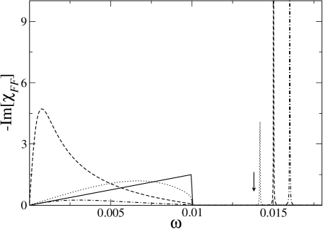
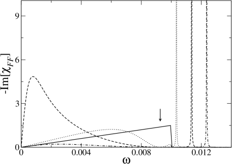
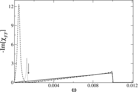
Figure 2: Imaginary part of the fermion-fermion density response function $-$Im$\chi_{FF}({\mathbf{k}},\omega)$ for $k=0.01\,k_{F}$ as a function of $\omega$ (in units of $\hbar k_{F}^{2}/m_{F}$) in a homogeneous ⁶Li-⁷Li mixture for various values for the coupling $a_{BF}$: the solid, dotted, dashed, and dash-dotted lines correspond to four equally spaced values of $|a_{BF}|$ from zero to the demixing or collapse point lying at $a_{BF}=7.9$ nm. The arrow marks the location of the Bogoliubov sound mode in the absence of boson-fermion interactions. The three panels from top to bottom correspond to the choices $c_{B}/v_{F}\simeq 1.4$, $c_{B}/v_{F}\simeq 0.92$ and $c_{B}/v_{F}\simeq 0.14$. The corresponding values of the particle densities (in units of $a_{ho}^{-3}$) are $n_{F}=8.9$ and $n_{B}=32555$, 14649, and 351.5 from top to bottom.

At increasing values of the boson-fermion coupling one must resort to a numerical solution of the RPA equations. Figure 2 shows the fermionic spectrum ${\rm Im}\chi_{FF}({\mathbf{k}},\omega)$ for various values of $g_{BF}$, the taking other parameters from the values at the center of the trap in a ⁶Li-⁷Li mixture Schreck et al. (2001) with equal trap frequencies $\omega_{F}=\omega_{B}=\omega_{0}=2\pi\times 1000\,$s^-1 and bosonic scattering length $a_{BB}=0.27$ nm. While in the RPA all four partial response functions $\chi_{\sigma\sigma^{\prime}}(\mathbf{k},\omega)$ share the same poles, we have chosen this spectrum because it shows most clearly the role of the fermionic particle-hole continuum.

We consider first the case $c_{B}>v_{F}$. As the gas approaches the instability points for demixing or collapse as given by Eq. (7), we observe a softening of the particle-hole spectrum until most of the oscillator strength is transferred to the bosonic mode at the point of collapse or demixing (see the first panel in Figure 2). In the case $c_{B}\lesssim v_{F}$ we observe that the boson-fermion interactions help to stabilize the bosonic mode, since mode repulsion pushes it out of the particle-hole continuum (see the second panel in Figure 2). This is not possible however in the case $c_{B}\ll v_{F}$, where the effect of boson-fermion hybridization is to break the particle-hole continuum into two parts (see the third panel in Figure 2). In this case as the system approaches the instability point it is the original bosonic mode which softens and broadens.

The softening of the spectrum is directly reflected in the partial “compressibilities”, obtained from the long wavelength limit of the static susceptibilities as

$$\chi_{\sigma\sigma^{\prime}}(k\rightarrow 0,\omega=0)=\int_{-\infty}^{\infty}\frac{d\omega^{\prime}}{\pi}\frac{{\rm Im}\chi_{\sigma\sigma^{\prime}}(k\rightarrow 0,\omega^{\prime})}{\omega^{\prime}}.$$ (24)

In the homogeneous mixture these quantities can be calculated analytically from the limiting behaviors of $\chi^{Bog}$ and $\chi^{0F}$:

$$\bar{\chi}(k\rightarrow 0,\omega=0)=\frac{1}{g_{BB}g_{FF}-g_{BF}^{2}}\left(\begin{array}[]{cc}-g_{BB}&g_{BF}\\ g_{BF}&-g_{FF}\end{array}\right).$$ (25)

From the above equation we immediately see that the RPA predicts a divergence in the compressibilities at the same instability points as obtained from static considerations. Alternatively, the instability point of the homogeneous mixture can be predicted from the emergence of unstable modes according to the condition

$$\lim_{\omega\rightarrow 0}\epsilon({\mathbf{k}},i\omega)=0$$ (26)

at long wavelengths.

Finally, from the form of the RPA solution in Eqs. (20) and (21) it is natural to define the effective fermion-fermion and boson-boson coupling as $g_{eff}^{FF}=g_{BF}^{2}\,\chi^{Bog}({\mathbf{k}},\omega)$ and $g_{eff}^{BB}=g_{BF}^{2}\,\chi^{0F}({\mathbf{k}},\omega)$, respectively Bijlsma et al. (2000); Heiselberg et al. (2000). From this point of view the instabilities occur when the effective interactions, which are negative in the limit $(k\rightarrow 0,\omega=0)$, overcome the Fermi pressure for the fermions and the boson-boson repulsions for the bosons.

V Spectra of a mesoscopic cloud in a trap

We consider now a mixture under external harmonic confinement, choosing for simplicity the spherically symmetric case $V_{ext}^{B,F}=m_{B,F}\omega_{0}^{2}r^{2}/2$ with the same trap frequency $\omega_{0}$ for the two atomic species. As for the homogeneous gas, we investigate how the spectrum of collective excitations is modified as the confined cloud moves toward demixing or collapse. Important differences arise from the presence of the confinement, under which both the Bogoliubov sound and the fermionic particle-hole spectrum are quantized. In particular the discrete energy levels depend on the static Hartree-Fock fields and shift as we vary the coupling strength, so that we know a priori that the spectra will not be symmetric under a change in the sign of $g_{BF}$.

For the finite system we follow the usual convention of evaluating the spectral strength functions $\chi_{\sigma\sigma^{\prime}}(\omega)$ Bertsch and Tsai (1975); Capuzzi and Hernández (2001), which are defined as

$$\chi_{\sigma\sigma^{\prime}}(\omega)=\int d^{3}r\int d^{3}r^{\prime}\,\delta U_{\sigma^{\prime}}^{*}(\mathbf{r})\,\chi_{\sigma\sigma^{\prime}}(\mathbf{r},\mathbf{r^{\prime}},\omega)\delta U_{\sigma}(\mathbf{r^{\prime}})$$ (27)

where $\delta U_{\sigma}(\mathbf{r})$ are the intensities of the time-dependent external potentials driving the two atomic species. In the case of spherical confinement these have the form $\delta U_{\sigma}(\mathbf{r})=f_{\sigma}(r)Y_{lm}(\hat{r})$ and correspondingly we can decompose the response functions into components of definite angular momentum,

$$\chi_{\sigma\sigma^{\prime}}({\mathbf{r}},{\mathbf{r}}^{\prime},\omega)=\sum_{l,m}\frac{4\pi}{2l+1}\chi^{l}_{\sigma\sigma^{\prime}}(r,r^{\prime},\omega)Y_{lm}(\hat{r})Y_{lm}^{*}(\hat{r}^{\prime}).$$ (28)

In these equations $Y_{lm}(\hat{r})$ are the spherical harmonic functions and $\hat{r}$ denotes the unit vector along $\mathbf{r}$.

Phase separation into the “egg” configuration or collapse has symmetry corresponding to $l=0$ and therefore we focus on the monopolar excitations of the type $\delta U_{\sigma}(\mathbf{r})=U_{0}\,(r/a_{ho})^{2}$. This type of perturbation can easily be produced in current experiments since it corresponds to just a modulation of the trap frequencies. In this case the strength function takes the form

$$\chi_{\sigma\sigma^{\prime}}^{l=0}(\omega)=U_{0}^{2}\int d^{3}r\int d^{3}r^{\prime}\,\frac{r^{2}}{a_{ho}^{2}}\,\frac{{r^{\prime}}^{2}}{a_{ho}^{2}}\,\chi_{\sigma\sigma^{\prime}}^{l=0}(r,r^{\prime},\omega).$$ (29)

We have obtained these RPA spectra by numerically solving the integro-differential problem posed by Eqs. (12)-(15) in conjunction with the determination of excited-state orbitals for the condensate and for the Fermi gas. A few points on the numerical solution are worth noting: (i) the orbitals $\psi_{i}$ and $\phi_{i}$ are discretized on a uniform mesh of about 250 points expanding to approximately twice the size of the density profiles; (ii) convergence is achieved both in the chemical potentials and in the respective energy spectrum; and (iii) for attractive boson-fermion coupling the numerical solution is computationally more demanding since a larger basis set is needed to properly describe the equilibrium density profiles as we approach the collapse.

V.1 Across demixing

We have calculated the RPA spectra of a mixture of ⁷Li and ⁶Li atoms Schreck et al. (2001) with trap frequency $\omega_{0}=2\pi\times 1000\,$s^-1, bosonic scattering length $a_{BB}=0.27$ nm, and a tunable $a_{BF}$ chosen to span the phase diagram from the mixed state to partially demixed states (as we shall see below, the spectrum shows a dynamical transition well before full separation). Experimentally the value of the boson-fermion scattering length can be tuned e.g. by using a Feshbach resonance.

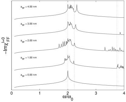
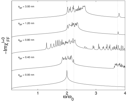
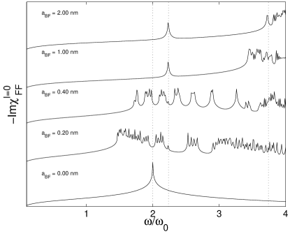
Figure 3: Spectrum of monopolar response (in log scale and arbitrary units) as a function of frequency $\omega$ (in units of $\omega_{0}$) for a boson-fermion mixture in harmonic confinement with $N_{F}=10^{4}$ and $N_{B}=10^{5}$ (top panel), $10^{6}$ (middle panel), and $2.4\times 10^{7}$ (bottom panel), for various values of $a_{BF}$ (in nm) as indicated in each panel. The vertical dotted lines indicate the frequency of fermionic (left) and bosonic (right) modes in the absence of boson-fermion coupling.

In Fig. 3 we show the imaginary part Im${\chi}_{FF}^{l=0}(\omega)$ of the strength function for $N_{F}=10^{4}$ and various values of $N_{B}$. In the absence of boson-fermion interactions the cloud responds to a monopolar excitation with only two well-defined modes, a purely fermionic one at frequency $\omega_{f}=2\,\omega_{0}$ Amoruso et al. (1999) and a purely bosonic one at frequency $\omega_{b}\simeq\sqrt{5}\,\omega_{0}$ Stringari (1996). The latter, of course, is not present in the fermionic spectrum for $a_{BF}=0$. Upon turning on the boson-fermion interactions the bosonic peak appears in the fermionic strength function with a considerable oscillator strength, showing that due to the boson-fermion coupling the fermionic cloud can oscillate in resonance with the bosons even in the collisionless regime. This “bosonic” mode moves to higher frequency as $a_{BF}$ is increased, analogously to what is found in the homogeneous mixture. A second “bosonic” peak also appears in the fermionic strength function, corresponding to a mode at $\omega_{b2}\simeq\sqrt{14}\,\omega_{0}$ in the absence of boson-fermion coupling. This $n=2$ mode is not excited by a monopolar perturbation in a pure bosonic cloud, but is excited in the mixture due to the dynamical coupling between bosons and fermions. Within the RPA the fermionic density fluctuations act as further perturbing fields on the bosons, and vice versa. .

For values of the frequency close to the original purely fermionic peak we observe a strong fragmentation of the strength function, most of which is already present at mean-field level in the Hartree-Fock fermionic spectrum. This fragmentation, which has also been reported for other choices of system parameters Capuzzi and Hernández (2001); Sogo et al. (2002), is due to boson-fermion interactions lifting the angular degeneracy of the single-particle levels for fermions in the trap. In addition to fragmentation we observe a softening of the original fermionic spectrum. The softening stops when the topology of the cloud changes, with the opening of a hole in the fermionic density at the trap center, although strong overlap of the two clouds is still present. This dynamical transition has also been found in the collisional regime Capuzzi et al. (2003) and occurs in both regimes at the same point, which is well described by the analytical expression (9). For larger values of the boson-fermion coupling the original fermionic component of the spectrum moves upward, again in analogy with the behavior of a trapped mixture in the collisional regime Capuzzi et al. (2003). This effect is intrinsically due to the harmonic confinement: at increasing $a_{BF}$ the fermion cloud forms a shell around the bosons with increasing average density and decreasing thickness, thus increasing its stiffness in response to the monopolar perturbation. In the homogeneous system instead the softening of the fermionic spectrum continues up to the point of full thermodynamic separation. The role of the number of bosons in the cloud is also evident from Figure  3.

As in Sec. IV, it is possible to monitor the softening or hardening of a part of the spectrum in the trapped cloud by looking at the “minus-one” moment of the monopolar spectral strength distribution. This spectral moment is specially sensitive to the low-frequency part of the spectrum and, owing to the Kramers-Kronig relations, yields the static limit $\chi_{\sigma\sigma^{\prime}}^{l=0}(\omega=0)$ of the strength function, thus defining four generalized compressibilities which measure the reaction of the cloud to a radial pressure exerted on a given component. In Fig. 4 (left panels) we show the fermionic compressibility $\chi_{FF}^{l=0}(\omega=0)$ both for positive and negative values of $g_{BF}$ and for three choices of the number of bosons. For positive $g_{BF}$ we observe an initial increase of $\chi_{FF}^{l=0}(\omega=0)$, followed by a slow decrease after the dynamical transition has taken place. The position of the maximum corresponds to the dynamical point of demixing in Eq. (9).

At variance from the homogeneous case, the four compressibilities in the trapped cloud have a nonsymmetric behavior for positive and negative values of the boson-fermion coupling. In particular this means that the compressibilities cannot be predicted by a simple local-density approach. For example, in the homogeneous gas one always finds a negative value of -$\bar{\chi}_{BF}(\omega=0)$ for $g_{BF}>0$ irrespectively of the actual values of the densities, whereas as is shown in Fig. 4 (right panels) this compressibility becomes positive in the confined cloud after the dynamical demixing point.

V.2 Towards collapse

We consider now the case of attractive boson-fermion interactions, choosing the trap parameters of the ⁶Li-⁷Li mixture as in the previous section. As is shown in the inset in Fig. 1, when the numbers of bosons and fermions are comparable the cloud can be found in a metastable state, while for larger numbers of bosons a wide stable region is present in the phase diagram. The collapse is reached at smaller values of $a_{BF}$ as the number of bosons is increased, as can be understood from the fact that the boson-mediated fermion-fermion attraction increases with $N_{B}$.

In the homogeneous gas the RPA spectra for attractive boson-fermion interactions coincide with those given in Fig. 2 for the case of repulsive interactions. This does not apply to the trapped mixture, as can already be seen from the compressibilities in Fig. 4. Contrary to the behavior of the homogeneous gas where the generalized compressibilities diverge at the instability points (see Eq. (25)), in the harmonic trap for negative values of $a_{BF}$ they decrease and for large numbers of bosons tend to vanish as the cloud approaches collapse. This is an indication that spectral weight is being transferred to high-frequency modes, and the effect becomes more dramatic as the number of bosons in the mixture is increased. In the limit $N_{B}\gg N_{F}$ the decrease of the fermion-fermion compressibility can be analytically predicted using a single-mode approximation (see the inset in Fig. 4). The details are given in Appendix A.

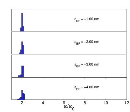
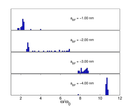
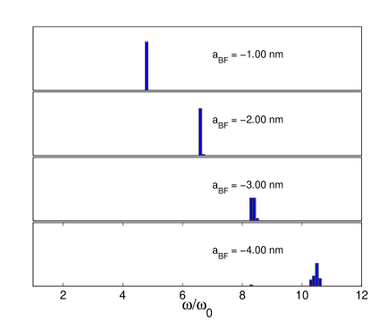
Figure 5: Hartree-Fock fermionic spectral functions (in arbitrary units) as functions of $\omega/\omega_{0}$ for $N_{F}=10^{4}$ and $N_{B}=10^{5}$ (top), $10^{6}$ (middle), and $2.4\times 10^{7}$, at various values of $a_{BF}$ as indicated in the panels.

A blue shift of the modes in the fermionic spectrum is found already at the Hartree-Fock level, as is illustrated in Fig. 5 by reporting the density $\rho_{2}(\varepsilon)$ of excited pairs,

$$\rho_{2}(\varepsilon)=\sum_{n,l}[f(\varepsilon_{n,l})-f(\varepsilon_{n+1,l})]\,\delta[\varepsilon-(\varepsilon_{n+1,l}-\varepsilon_{n,l})]$$ (30)

at increasing $N_{B}$ for $N_{F}=10^{4}$ and various values of $a_{BF}$. In Eq. (30) we have chosen only the pairs with $\Delta l=0$ to obtain a monopolar particle-hole excitation spectrum, with $\Delta n=1$ since this gives the most important contribution at low frequencies.

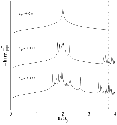
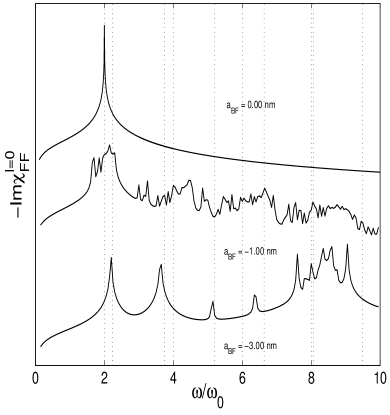
Figure 6: Spectrum of monopolar response (in log scale and arbitrary units) as a function of frequency $\omega$ (in units of $\omega_{0}$) for a boson-fermion mixture in harmonic confinement with $N_{F}=10^{4}$ and $N_{B}=10^{5}$ (left panel) and $10^{6}$ (right panel), at various values of $a_{BF}$ (in nm) as indicated in each panel. The vertical dotted lines indicate the frequency of fermionic (at integer multiples of $2\omega_{0}$) and bosonic modes in the absence of boson-fermion interactions.

The spectra resulting from a full RPA calculation of the monopolar fermion-fermion response in the region of boson-fermion attractions are shown in Figs. 6 and 7. When the numbers of bosons and fermions are comparable we observe a shift of the pure fermionic peak towards lower frequencies. We interpret this shift as being associated with the lifting of the degeneracy of the single-particle Hartree-Fock spectrum by boson-fermion attractions, which allow transitions between states that are closer in energy. At increasing values of $N_{B}$ we find instead that the fermionic mode is blue-shifted by a much larger amount, as a result of the static Hartree field of the bosons. The amount of the shift can be predicted analytically in the limit $N_{B}\gg N_{F}$, where the interactions with the bosons simply renormalize the trap frequency (see Appendix A). In the same limit the bosonic modes are almost unaffected by the interactions with the fermions, as the fermionic Hartree field becomes almost negligible for the bosons.

VI Summary and concluding remarks

In summary, in this paper we have studied how the mutual interactions of bosons and fermions affect the spectrum of collective excitations of a dilute boson-fermion mixture in the collisionless regime as the mixture goes towards either demixing or collapse. To this purpose we have used the Random-Phase approximation, which is most suited in the dilute regime since it accounts correctly for the limit of small couplings and generally conserves the $f$-sum rule. We have studied both a homogeneous mixture and a mixture in isotropic harmonic confinement, where new effects arise due to the static mean-field interactions. We have indeed found that both the boson-fermion coupling and the confinement strongly change the spectra of collective excitations. Our main results are as follows.

First of all, in the presence of boson-fermion interactions the excitation of one component of the mixture will set into motion also the other component. There also is hybridization of the excitation modes, e.g. the fermionic component can also oscillate in resonance with the bosonic cloud at the frequency of a bosonic mode and vice versa.

In the homogeneous gas we observe qualitatively different behaviors depending on the ratio between the Bogoliubov sound velocity $c_{B}$ and the Fermi velocity $v_{F}$. In the case $c_{B}>v_{F}$ at increasing values of the boson-fermion coupling we find mode repulsion between the broad particle-hole continuum and the Bogoliubov sound, and the fermionic spectrum softens as the gas approaches either instability point. When $c_{B}$ is just below $v_{F}$ the Bogoliubov sound is damped at low couplings, but a “revival” of this mode can take place as the boson-fermion interactions are increased. Softening and damping of the bosonic mode is instead observed when $c_{B}\ll v_{F}$. Within the RPA we have also derived a dynamical condition for the two instabilities, which coincides with that obtained by studying the linear stability of the mean-field energy functional.

In the trapped system we have studied the $l=0$ monopolar excitations. While in the absence of interactions the spectrum of density fluctuations shows only two sharp and independent modes, the boson-fermion coupling induces fragmentation of the original fermionic mode, revealing the presence of many occupied single-particle levels in the Fermi sphere. At increased repulsive couplings we observe a softening of the spectrum up to the point where the topology of the fermionic cloud changes by the formation of a hole at its center. The spectrum is then shifted to higher values of the frequencies at larger values of $a_{BF}$. For negative values of the coupling we observe some frequency decrease for comparable numbers of bosons and fermions, but as the number of bosons increases the static Hartree field of the bosons drives a sizable blue shift of the fermionic modes.

From the comparative analysis of the collective excitation spectra of the mixture in the homogeneous state and inside a trap we have learnt that the inhomogeneous trap potential can change quite drastically the physical picture, since the instabilities are approached along thermodynamically different routes. In the homogeneous gas one works at fixed average particle densities, while the confined cloud must be treated at fixed external confinement. We have found that the partial compressibilities cannot be described by a local-density picture, and while they are expected to diverge in the homogeneous gas on approaching the instability points, in the trap they saturate to finite values as the component of the mixture are spatially separating and vanish as collapse is approached. This suggests that a description of boson-induced fermion-fermion interactions, e.g. in the study of the instability against pairing, may also be affected by the confinement.

In this work we have neglected the static and dynamical effects of correlations and the quantum depletion of the condensate Albus et al. (2002); Viverit and Giorgini (2002). These should become important in the proximity of collapse as the gas densities increase. The effects of temperature may also be of interest, with the thermal depletion of the condensate and the blurring of the Fermi surface yielding, for instance, damping of the Bogoliubov sound. Finally, new dynamical effects may arise when the components of the trapped mixture have very different atomic masses and will be studied elsewhere.

Appendix A Single-pole model for the trapped mixture

We derive in this Appendix a single-pole model to describe the partial fermion-fermion compressibility for attractive boson-fermion interactions in the limit of large boson numbers. This model accounts rather well for our numerical results and shows how the inhomogeneous harmonic confinement in combination with the boson-fermion coupling can give rise to a completely different behavior in the compressibility relative to the homogeneous case.

In the limit $N_{B}\gg N_{F}$ the dynamical coupling between bosons and fermions is quite small, but the fermionic density is largely affected by the static mean field of the bosons. The bosonic equilibrium profile is only weakly affected by the presence of the fermions, so that in the Thomas Fermi approximation we can write $n_{B}(\mathbf{r})=[\mu_{B}-V_{ext}^{B}(r)]\theta(R_{B}-r)/g_{BB}$ with $R_{B}=(2\mu_{B}/m_{B}\omega_{0}^{2})^{1/2}$. In these conditions it is useful to introduce an effective potential acting on the fermions as Vichi et al. (2000)

$$V_{eff}^{F}(r) = \frac{1}{2}m_{F}\omega_{0}^{2}r^{2}+g_{BF}n_{B}(r)$$ (31)

$$\simeq \frac{1}{2}m_{F}\omega_{0}^{2}r^{2}\left[1-\frac{m_{B}g_{BF}}{m_{F}g_{BB}}\theta(R_{B}-r)\right]+\frac{g_{BF}}{g_{BB}}\mu_{B}\theta(R_{B}-r).$$

For the choice $N_{B}=2.4\times 10^{7}$ and $N_{F}=10^{4}$ the bosonic and fermionic clouds have the same radii, so that the effective potential is seen by the fermions at all $r$ and acts as a harmonic trap with renormalized frequency $\tilde{\omega}=\omega_{0}[1-(m_{B}g_{BF})/(m_{F}g_{BB})]^{1/2}$.

An analytical estimate of the compressibility can be obtained by making a single-pole approximation on the fermion-fermion strength function

$${\rm Im}\chi_{FF}(\omega)=-\frac{1}{\pi}A\delta(\omega-\omega_{e})$$ (32)

where for monopolar excitations we take $\omega_{e}=2\tilde{\omega}$. The oscillator strength $A$ is determined from the $f$-sum rule, which for a trapped system reads Bruun (2001)

$$-\int\frac{d\hbar\omega}{\pi}\,\hbar\omega\,{\rm Im}\chi_{FF}(\omega)\equiv M_{1}=\frac{\hbar^{2}}{m_{F}}\int d^{3}r|\nabla\delta U_{F}(r)|^{2}n_{F}(r)$$ (33)

In our case $\delta U_{F}=U_{0}(r/a_{ho})^{2}$ and the RHS of Eq. (33) is determined by the mean square radius of the equilibrium fermionic density: $M_{1}=4\hbar\omega_{0}U_{0}^{2}\langle r^{2}\rangle/a_{ho}^{2}(m_{B}/m_{F})$. This is readily evaluated from the Thomas-Fermi approximation $n_{F}(r)=(6\pi^{2})^{-1}[(2m_{F}/\hbar^{2})(\mu_{F}-m_{F}\tilde{\omega}^{2}r^{2}/2)]^{3/2}\theta(\mu_{F}-m_{F}\tilde{\omega}^{2}r^{2}/2))$, where for $R_{F}\simeq R_{B}$ the chemical potential is simply given by $\mu_{F}=\hbar\tilde{\omega}(6N_{F})^{1/3}$. We therefore obtain for the oscillator strength the value

$$A=3^{4/3}2^{-2/3}N_{F}^{4/3}\left(\frac{\omega_{0}}{\tilde{\omega}}\right)^{2}U_{0}^{2}\left(\frac{m_{B}}{m_{F}}\right)^{2}.$$ (34)

Finally, from the imaginary part of the strength function we can calculate the compressibility by means of the Kramers-Kronig relation, with the result

$$\hbar\omega_{0}\,\chi_{FF}(\omega=0)=\frac{3^{4/3}2^{1/3}}{2\pi^{2}}N_{F}^{4/3}U_{0}^{2}\left(\frac{\omega_{0}}{\tilde{\omega}}\right)^{3}\left(\frac{m_{B}}{m_{F}}\right)^{2}.$$ (35)

This depends on $a_{BF}$ through $\tilde{\omega}$ and gives a quantitative agreement with the numerical calculations (see the inset in Fig 4).

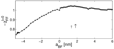
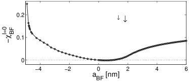
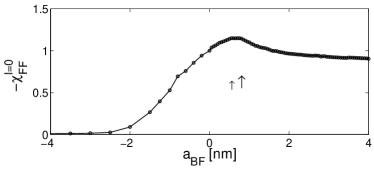
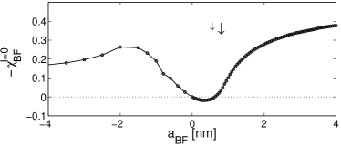
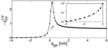
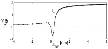
Figure 4: Generalized compressibilities (in units of $\chi_{FF}^{l=0}$ at $a_{BF}=0$) of a boson-fermion mixture in harmonic confinement as functions of the boson-fermion scattering length $a_{BF}$ (in nm) for $N_{F}=10^{4}$ and $N_{B}=10^{5}$ (top), $10^{6}$ (middle), and $2.4\times 10^{7}$ (bottom). The small and large arrows indicate the points of onset of partial demixing and of the dynamical transition from Eqs. (8) and (9), respectively. The lines are a guide to the eye. The inset shows an enlargement of the region with $a_{BF}<0$ in comparison with the analytical predictions from Eq. (35) (dashed line).

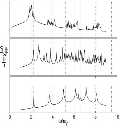
Figure 7: Spectrum of monopolar response (in log scale and arbitrary units) as a function of frequency $\omega$ (in units of $\omega_{0}$) for a boson-fermion mixture in harmonic confinement with $a_{BF}=-2$ nm and $N_{F}=10^{4}$ at various values of $N_{B}$: $N_{B}=10^{5}$ (top), $N_{B}=10^{6}$ (middle) and $N_{B}=2.4\times 10^{7}$ (bottom). The vertical lines indicate the frequencies of fermionic modes (dotted lines) and bosonic modes (dot-dashed lines) in the absence of boson-fermion interactions. For the above sets of parameters thermodynamic collapse is predicted to occur at $a_{BF}\simeq-4.9$ nm for $N_{B}=10^{5}$, $-4.4$ nm for $N_{B}=10^{6}$, and $-4.0$ nm for $N_{B}=2.4\times 10^{7}$.

References

- Schreck et al. (2001) F. Schreck, L. Khaykovich, K. L. Corwin, G. Ferrari, T. Bourdel, J. Cubizolles, and C. Salomon, Phys. Rev. Lett. 87, 080403 (2001).
- Goldwin et al. (2002) J. Goldwin, S. B. Papp, B. DeMarco, and D. S. Jin, Phys. Rev. A 65, 021402 (2002).
- Hadzibabic et al. (2002) Z. Hadzibabic, C. A. Stan, K. Dieckmann, S. Gupta, M. W. Zwierlein, A. Görlitz, and W. Ketterle, Phys. Rev. Lett. 88, 160401 (2002).
- Roati et al. (2002) G. Roati, F. Riboli, G. Modugno, and M. Inguscio, Phys. Rev. Lett. 89, 150403 (2002).
- Modugno et al. (2002) G. Modugno, G. Roati, F. Riboli, F. Ferlaino, R. J. Brecha, and M. Inguscio, Science 297, 2240 (2002).
- Ferlaino et al. (2003) F. Ferlaino, R. J. Brecha, P. Hannaford, F. Riboli, G. Roati, G. Modugno, and M. Inguscio, J. Opt. B: Quantum Semiclass. Opt. 5, S3 (2003).
- Mølmer (1998) K. Mølmer, Phys. Rev. Lett. 80, 1804 (1998).
- Akdeniz et al. (2002a) Z. Akdeniz, A. Minguzzi, P. Vignolo, and M. P. Tosi, Phys. Rev. A 66, 013620 (2002a).
- Akdeniz et al. (2002b) Z. Akdeniz, P. Vignolo, A. Minguzzi, and M. P. Tosi, J. Phys. B 35, L105 (2002b).
- Miyakawa et al. (2001) T. Miyakawa, T. Suzuki, and H. Yabu, Phys. Rev. A 64, 033611 (2001).
- Efremov and Viverit (2002) D. V. Efremov and L. Viverit, Phys. Rev. B 65, 134519 (2002).
- Yip (2001) S. K. Yip, Phys. Rev. A 64, 023609 (2001).
- Search et al. (2002) C. P. Search, H. Pu, W. Zhang, and P. Meystre, Phys. Rev. A 65, 063615 (2002).
- Viverit and Giorgini (2002) L. Viverit and S. Giorgini, Phys. Rev. A 66, 063604 (2002).
- Miyakawa et al. (2000) T. Miyakawa, T. Suzuki, and H. Yabu, Phys. Rev. A 62, 063613 (2000).
- Liu and Hu (2003) X.-J. Liu and H. Hu, Phys. Rev. A 67, 023613 (2003).
- Minguzzi and Tosi (2000) A. Minguzzi and M. P. Tosi, Phys. Lett. A 268, 142 (2000).
- Capuzzi and Hernández (2001) P. Capuzzi and E. S. Hernández, Phys. Rev. A 64, 043607 (2001).
- Sogo et al. (2002) T. Sogo, T. Miyakawa, T. Suzuki, and H. Yabu, Phys. Rev. A 66, 013618 (2002).
- Capuzzi and Hernández (2002) P. Capuzzi and E. S. Hernández, Phys. Rev. A 66, 035602 (2002).
- Capuzzi et al. (2003) P. Capuzzi, A. Minguzzi, and M. P. Tosi, Phys. Rev. A (2003), in press.
- Viverit et al. (2000) L. Viverit, C. J. Pethick, and H. Smith, Phys. Rev. A 61, 053605 (2000).
- Roth (2002) R. Roth, Phys. Rev. A 66, 013614 (2002).
- Pines and Nozières (1966) D. Pines and P. Nozières, The Theory of Quantum Liquids, vol. I (Benjamin, New York, 1966).
- Fetter and Walecka (1971) A. L. Fetter and J. D. Walecka, Quantum Theory of Many-Particle Systems (McGraw-Hill, New York, 1971).
- Bijlsma et al. (2000) M. J. Bijlsma, B. A. Heringa, and H. T. C. Stoof, Phys. Rev. A 61, 053601 (2000).
- Heiselberg et al. (2000) H. Heiselberg, C. J. Pethick, H. Smith, and L. Viverit, Phys. Rev. Lett. 85, 2418 (2000).
- Bertsch and Tsai (1975) G. F. Bertsch and S. F. Tsai, Phys. Rep. 18, 125 (1975).
- Amoruso et al. (1999) M. Amoruso, I. Meccoli, A. Minguzzi, and M. P. Tosi, Eur. Phys. J. D 7, 441 (1999).
- Stringari (1996) S. Stringari, Phys. Rev. Lett. 77, 2360 (1996).
- Albus et al. (2002) A. P. Albus, S. A. Gardiner, F. Illuminati, and M. Wilkens, Phys. Rev. A 65, 053607 (2002).
- Vichi et al. (2000) L. Vichi, M. Amoruso, A. Minguzzi, S. Stringari, and M. P. Tosi, Eur. Phys. J. D 11, 335 (2000).
- Bruun (2001) G. M. Bruun, Phys. Rev. A 63, 043408 (2001).