Thermodynamic perturbation theory of the phase behaviour of colloid / interacting polymer mixtures

Abstract

We use thermodynamic perturbation theory to calculate the free energies and resulting phase diagrams of binary systems of spherical colloidal particles and interacting polymer coils in good solvent within an effective one-component representation of such mixtures, whereby the colloidal particles interact via a polymer-induced depletion potential. MC simulations are used to test the convergence of the high temperature expansion of the free energy. The phase diagrams calculated for several polymer to colloid size ratios differ considerably from the results of similar calculations for mixtures of colloids and ideal (non-interacting) polymers, and are in good overall agreement with the results of an explicit two-component representation of the same system, which includes more than two-body depletion forces.

I Introduction

The structure, rheology and phase behaviour of sterically stabilized colloidal dispersions are strongly affected by the presence of non adsorbing polymer. Nearly fifty years ago Asakura and Oosawa realized that finite concentrations of polymer coils would induce an effective attraction between colloidal particles, of essentially entropic origin, the so-called depletion interaction AO . Since the initial colloid-polymer Hamiltonian involves only repulsive interactions between all pairs of particles, the polymer-induced effective attraction between colloids, which results from tracing out the polymer degrees of freedom, was referred to as “attraction through repulsion” by A. Vrij. For non-interacting (ideal) polymers, the range of the depletion attraction is independent of polymer concentration, and close to the polymer radius of gyration $R_{g}$, while the depth of the attractive well, when two colloids touch, is proportional to polymer concentration. Consequently, one expects that for sufficiently high concentration, and for not too small size ratio $q=R_{g}/R_{c}$ (where $R_{c}$ is the radius of the spherical colloids), the effective attraction may drive a depletion-induced phase separation into colloid-rich (“liquid”) and colloid-poor (“gas”) colloidal dispersions, similar to condensation in simple fluids. This phase transition, which is in fact a colloid-polymer demixing transition, was investigated by Gast et al. gast , who first calculated the phase diagram from thermodynamic perturbation theory. Their findings were later confirmed by the Monte-Carlo (MC) simulations of Meijer and Frenkel meijer , and the free volume theory of Lekkerkerker et al. lekk . The predicted phase diagrams agree qualitatively with experimental findings for various colloid / polymer mixtures experiments ; ilett .

More recently the question was raised of how interactions between polymer coils would affect the phase behaviour compared to that of ideal polymers warren ; fuchs ; PRL89 ; aarts ; schmidt . The early theoretical investigations into the problem were made at the two-component level, involving an explicit consideration of the polymer coils. However very recently the depletion-driven effective pair-potential between two colloidal particles in a bath of interacting polymers in good solvent, modelled as self-avoiding walk (SAW) polymers, was calculated by MC simulations JCP117 . A simple analytic form, with coefficients determined by the SAW polymer osmotic equation of state and surface tension, yields excellent agreement with the simulation data over a wide range of polymer to colloid size ratio $q$, and polymer concentrations JCP117 .

In this paper we use thermodynamic perturbation theory simplliq to calculate the phase diagram of mixtures of hard sphere colloids and interacting polymers within the effective one-component representation, whereby the colloidal particles interact via the above-mentioned depletion potential induced by the SAW polymers. The results of these calculations can be directly compared to the predictions of recent MC simulations of the two-component representation of the same system PRL89 , which agree quantitatively with recent experiments ramak . Any discrepancies between the phase diagrams obtained within the effective one-component and two-component representations can then be traced back to more-than-two-body depletion interactions between colloidal particles, which are automatically included in the latter representation, but are of course neglected in the pairwise additive effective one-component picture considered in the present paper.

Thermodynamic perturbation theory was previously applied to mixtures of hard sphere colloids and ideal polymers within the effective one-component representation by Gast et al. gast , and improved by Dijkstra et al. dijkstra . Similar calculations were recently published for mixtures of colloids and star polymers for several functionalities $f$ (where $f$ is the number of identical arms of the star polymer connected at the centre), again within an effective one-component representation, as well as within the two-component description dzubiella . Star polymers are particularly instructive depletants, since upon varying the functionality, they change continuously from linear polymer ($f=2$) to hard-sphere like behaviour ($f\rightarrow\infty$). The phase diagrams obtained in ref. dzubiella for $f=2$ are thus, in principle directly comparable to the results presented in this paper. Such a comparison will be made in section $4$, but is only tentative, since the calculations in ref. dzubiella neglect the polymer concentration-dependence of the effective colloid-polymer and the polymer-polymer interactions which are not negligible PRL89 ; JCP114 ; macromol .

II One and two-component representations

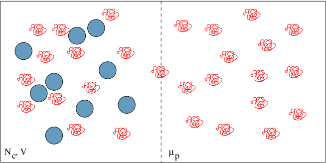
Figure 1: Schematic representation of the semi-grand canonical ensemble. $N_{c}$ colloidal particles in a volume $V$ are in osmotic equilibrium with a polymer reservoir of fixed chemical potential $\mu_{p}$.

Consider a system of $N_{c}$ spherical colloidal particles of radius $R_{c}$, in a bath of linear polymers which are in equilibrium with a polymer reservoir of fixed chemical potential $\mu_{p}$. The corresponding semi-grand canonical description is schematically represented in figure 1. The colloidal particles interact via the standard hard sphere potential, while each polymer is made up of $L$ monomers or segments; segments from the same or different chains are not allowed to overlap. In good solvent, this excluded volume constraint is the only monomer-monomer interaction and for sufficiently large $L$, where chemical details become irrelevant, the interacting polymers may be accurately modelled by self avoiding walks on a three-dimensional lattice. The monomers, moreover, are not allowed to penetrate the hard sphere colloids. At finite colloid and polymer concentrations, such a binary mixture of hard spheres and interacting polymers poses a formidable problem to theoreticians and simulators alike.

One coarse-graining strategy which has proved very successful is to trace out individual monomer degrees of freedom in the “polymers as soft colloids” paradigm, whereby the total interaction between two polymer coils, averaged over all monomer configurations, reduces to an effective (entropic) interaction between their centres of mass, which depends on polymer concentration JCP114 . Similarly, one can trace out the monomer degrees of freedom, to derive a state-dependent effective interaction between the hard sphere colloids and the centres of mass of the polymer coils JCP114 ; macromol . This coarse-graining procedure, which amounts to a reduction of the number of degrees of freedom of each polymer from $\mathcal{O}(L)$ to $3$, leads to a two-component representation of “hard” and effective “soft” colloids, which has been exploited in recent MC simulations to determine the phase diagram of colloid / interacting polymer mixtures for several size ratios $q$ PRL89 . However, following the Asakura-Oosawa (AO) strategy for non-interacting polymers, one can carry the coarse-graining procedure one step further, by eliminating the polymer degrees of freedom altogether and determining the resulting depletion interactions between the colloidal particles. If this procedure is carried out in the semi-grand canonical ensemble, the total effective interaction energy between $N_{c}$ colloidal particles for any configuration $\overrightarrow{r}^{N_{c}}$ is:

$$V_{cc}^{eff}(\vec{r}^{N_{c}})\;\equiv\;V_{cc}(\vec{r}^{N_{c}})-k_{B}\,T\;{\rm ln}<{\rm exp}[-\beta V_{cp}]>_{\mu_{p},V,T}(\vec{r}^{N_{c}})$$ (1)

where $V_{cc}$ is the direct colloid-colloid interaction energy, while $V_{cp}$ is the total colloid-polymer interaction; the brackets denote a grand-canonical average over polymer degrees of freedom at fixed polymer chemical potential, volume and temperature, and a given colloid configuration. In the model under consideration, $V_{cc}$ and $V_{cp}$ are the colloid-colloid and colloid-monomer excluded volume interactions, which are pair-wise additive. The depletion interactions between the $N_{c}$ colloidal particles are given by the second term on the r.h.s. of Eq. (1) and are not, a priori, pair-wise additive. However, for sufficiently low colloid concentration, or small size ratio $q$, the pair-wise additive contribution dominates.

II.1 Depletion potential for interacting polymers

The depletion pair potential between an isolated pair of colloidal spheres has been determined as a function of the centre-to-centre distance, and over a range of interacting polymer concentrations covering the dilute and semi-dilute regimes, in ref. JCP117 . The resulting depletion pair potential is accurately reproduced by the following simple semi-empirical form, inspired by the Derjaguin approximation JCP117 :

$$\beta v_{s}(r)=\begin{cases}-\pi\,R_{c}\,\gamma_{w}(\rho)\,D_{s}(\rho)\left(1-\frac{x}{D_{s}(\rho)}\right)^{2}&;\quad 0\;\leq x\;\leq D_{s}(\rho)\;,\\ 0\quad{\rm otherwise}\end{cases}$$ (2)

$r$ is the centre-to-centre separation, while $x=r-2R_{c}$ is the surface-to-surface distance between the colloids; $\gamma_{w}(\rho)$ is the polymer surface tension near a planar wall, a function of polymer bulk concentration $\rho=\rho_{b}$ determined in ref. JCP116 for SAW polymers; $D_{s}(\rho)$ is the range of the depletion potential given, according to ref. JCP117 , by:

$$D_{s}(\rho)=\frac{2\gamma_{w}(\rho)}{\Pi(\rho)}\frac{R_{AO}^{eff}(q)}{R_{AO}^{eff}(q\rightarrow 0)}$$ (3)

where $\Pi(\rho)$ is the osmotic pressure of the interacting polymers taken from renormalization group calculations oono , namely:

$$\Pi(\rho)=\rho\,Z(\alpha\phi)$$ (4a)

where $$\alpha=2.55 \phi=4\pi\rho R_{g}^{3}/3 R_{g} \rho=0$$, , is the polymer radius of gyration at zero density (), and

$$Z(x)=1+\frac{x}{2}{\rm exp}\left[0.309\times[(1-\frac{1}{x^{2}}){\rm ln}(1+x)+\frac{1}{x}]\right]$$ (4b)

The second fraction on the r.h.s of (3) accounts for finite curvature of the colloid surface, as estimated approximately from the AO model for ideal polymers JCP116 :

$$\frac{R_{AO}^{eff}(q)}{R_{g}}=\frac{1}{q}\left(\left(1+\frac{6}{\sqrt{\pi}}q+3q^{2}\right)^{\frac{1}{3}}-1\right)\;,$$ (5)

which reduces to $2/\sqrt{\pi}$ in the limit $q\rightarrow 0$.

II.2 Depletion potential for ideal polymers

For comparative purposes, we also consider the depletion pair potential induced by ideal polymers. Meijer and Frenkel meijer showed that to a good approximation this is well represented by the Asakura-Oosawa form AO :

$$\beta v_{id}(r)=\begin{cases}-\frac{4\pi}{3}\rho\sigma^{3}\left\{1-\frac{3}{4}\frac{r}{\sigma}+\frac{1}{16}\left(\frac{r}{\sigma}\right)^{3}\right\}&;\;2\,R_{c}\leq r\leq\;2\sigma,\\ 0&{\rm otherwise}\end{cases}$$ (6)

where $\sigma=R_{c}+R_{AO}^{eff}$ is the radius of a sphere around the colloids from which the interpenetrable polymers are excluded, but with an effective $R_{AO}^{eff}$ calculated from the insertion free energy of a single colloid in a bath of ideal polymer. The radius is given by eq. (5) JCP116 ; for a hard wall it reduces to $2/\sqrt{\pi}\approx 1.128$, while it monotonically decreases for increasing size ratio $q$ since the polymer can deform around the spherical colloid. For the size ratios considered here the curvature effects are small, on the order of a few $\%$ aarts .

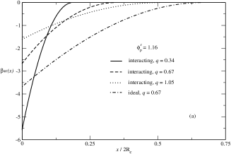
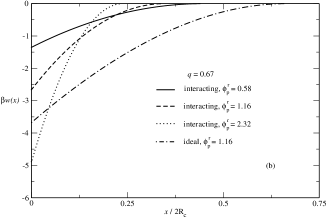
Figure 2: Depletion potential between two colloids as a function of the surface to surface distance, shown for interacting polymers ($w=v_{s}$ from eq. (2)) characterised by $q=0.34,0.67$ and $1.05$, for $\phi_{p}^{r}=1.16$ (a), and by $\phi_{p}^{r}=0.58,1.16$ and $2.32$ for $q=0.67$ (b). The dashed lines indicate the ideal potential ($w=v_{id}$ from eq. (6)) for the intermediate cases. For a given $\phi_{p}^{r}$ and $q$, $v_{id}(r)$ is always more attractive than $v_{s}(r)$.

The two pair potentials (2) and (6) are always attractive. For interacting polymers the range decreases with increasing polymer concentration $\rho$, while the latter is constant for ideal polymers. Furthermore, at any given $\rho$, the depth of $v_{s}(r)$ is always less than that of $v_{id}(r)$, so that the depletion attraction induced by interacting polymers is weaker than for ideal polymers. Representative examples of the depletion potentials (2) are shown in figure 2.

III Free energy calculations

Our objective is to draw phase diagrams of colloid / polymer mixtures in the ($\eta_{c}$,$\phi_{p}^{r}$) plane, where $\eta_{c}=4\pi\rho_{c}R_{c}^{3}/3$ is the colloid packing fraction, while $\phi_{p}^{r}=4\pi\rho_{p}^{r}R_{g}^{3}/3$ is the ratio of the polymer density in the reservoir ($r$) over the overlap density $\rho_{p}^{*}=3/4\pi R_{g}^{3}$; the latter conventionally separates the dilute ($\rho_{p}<\rho_{p}^{*}$) and the semi-dilute ($\rho_{p}>\rho_{p}^{*}$) regimes. To this end we need to calculate the free energies of the various phases. Within the semi-grand canonical ensemble the required free energy is related to the Helmholtz free energy $F_{c}(N_{c},N_{p},V,T)$ by a Legendre transformation:

$$F(N_{c},\phi_{p}^{r},V,T)=F(N_{c},\mu_{p},V,T)=F_{c}(N_{c},N_{p},V,T)-\mu_{p}N_{p}$$ (7)

Since the colloidal particles interact via a hard sphere repulsion and an effective, depletion-driven attraction, the natural way forward is to calculate the free energies of the various phases from thermodynamic perturbation theory, using the well-documented hard sphere fluid as a reference system simplliq . To second order in the high-temperature expansion:

$$F = F_{0}+F_{1}+F_{2}$$ (8)

$$= F_{0}+\left<W_{N_{c}}\right>_{0}+\frac{\beta}{2}\left[\left<W_{N_{c}}^{2}\right>_{0}-\left<W_{N_{c}}\right>_{0}^{2}\right]$$

where $F_{0}=F_{0}(N_{c},V,T)$ is the free energy of the hard sphere fluid, $\left<...\right>_{0}$ denotes an average over the reference system configurations, and $W_{N_{c}}$ is the perturbation potential energy:

$$W_{N_{c}}=\sum_{i<j}^{N_{c}}w(r_{ij})$$ (9)

with $r_{ij}=|\vec{r}_{i}-\vec{r}_{j}|$, the distance between the centres of colloids $i$ and $j$; $w=w(r;\phi_{p}^{r})$ is the polymer concentration-dependent depletion potential (2) for interacting polymers ($w=v_{s}$) or (6) for non-interacting polymers ($w=v_{id}$). We stress that within the semi-grand canonical description the depletion potential must be calculated for the polymer density in the reservoir, which is unequivocally determined by fixing the chemical potential $\mu_{p}$.

$F_{0}$ in eq. (8) is calculated from the Carnahan and Starling equation of state for the hard sphere fluid CS while for the hard sphere solid we adopt Hall’s equation of state hall . $F_{1}$ is easily expressed in terms of the hard sphere pair distribution function $g_{0}(r)$ for which we adopted the Verlet-Weis parametrisation in the fluid VW , and the form proposed by Kincaid and Weis for the FCC solid phase KW . The calculation of $F_{2}$ involves three and four-body contributions of the reference system. We have adopted the approximate expression due to Barker and Henderson barkerhend , which only involves the pair distribution function and the compressibility of the reference system. Gathering results:

$$\frac{\beta F}{N_{c}}=\frac{\beta F_{0}}{N_{c}}+\frac{1}{2}\beta\rho_{c}\int d^{3}r\,g_{0}(r)\,w(r)-\frac{1}{4}\left(\frac{\partial\rho_{c}}{\partial p}\right)_{0}\beta\rho_{c}\int d^{3}r\,g_{0}(r)\,w^{2}(r)\,.$$ (10)

Note that in the solid phase, $g_{0}(r)$ is the orientationally-averaged pair distribution function.

In order to assess the accuracy of $F_{2}$ and the convergence of the perturbation series (10), we have carried out MC simulations to compute explicitly the fluctuation term in eq. (8), which is approximated by the last term in eq. (10), as well as the total excess free energy. The latter is most conveniently calculated by the standard $\lambda$-integration procedure simplliq , whereby the depletion-induced perturbation $W_{N_{c}}$ is gradually switched on, resulting in:

$$F(\lambda=1)=F(\lambda=0)+\int_{0}^{1}\left<W_{N_{c}}\right>_{\lambda}d\lambda$$ (11)

where $F(\lambda=1)$ is the required free energy of the fully interacting colloid / polymer mixture, $F(\lambda=0)\equiv F_{0}$ is the free energy of the hard sphere reference system, and $\left<W_{N_{c}}\right>_{\lambda}$ is the statistical average of the perturbation weighted by the Boltzmann factor appropriate for a system of particles interacting via the hard sphere repulsion and the partially switched on depletion potential $\lambda w(r)$. The calculation of the free energy $F$ hence involves several MC simulations to determine $\left<W_{N_{c}}\right>_{\lambda}$ for a series of discrete values of $\lambda$PR184 , typically $\lambda=n\times 0.05$ ($1\leq n\leq 20$).

The convergence of the perturbation series (10) is illustrated in figure 3 for the depletion potential (2) and a size ratio $q=0.67$. As expected, the convergence of the series is faster when the size ratio $q$ is larger, the polymer concentration is lower and the colloid packing fraction higher.

The accuracy of each term in the series, and of the truncated sum, were tested by MC simulations of periodic samples of $N_{c}=108$ colloidal particles. Representative results are presented in tables I and II. Table I shows that values of $F_{1}$ from eq. (10) are very close to the simulation data, both for the fluid and the solid. The Barker-Henderson approximation underestimates the absolute value of $F_{2}$, by less than a factor of two in the fluid phase, and by a much larger factor in the FCC crystal phase, where it is totally inadequate. However, as shown in Table II, the sum of the first three terms of the perturbation series (10) yields a total free energy which is surprisingly close to the “exact” MC results from the $\lambda$-integration. Similar comparisons show that the predictions of perturbation theory are very reliable both for larger and for somewhat smaller values of $q$ (say for $q\gtrsim 0.3$), but that the predictions rapidly deteriorate for small $q$, corresponding to narrow potential wells, as expected. This failure will be illustrated in the case $q=0.1$ at the end of the following section.

IV Phase diagrams

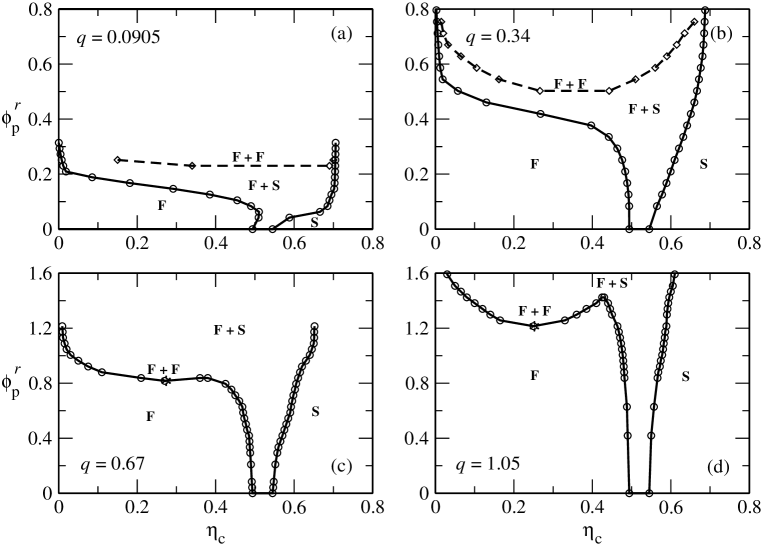
Figure 4: Phase diagrams of colloid / interacting polymer mixtures as obtained from perturbation theory for the effective one component system with size ratios (a) $q=R_{g}/R_{c}=0.0905$, (b) $q=0.34$, (c) $q=0.67$, and (d) $q=1.05$, in the plane of the colloid packing fraction $\eta_{c}$ and the polymer concentration $\phi_{p}^{r}$ in the reservoir. F and S denote the stable fluid and solid (FCC) phases. F + S and F + F denote the stable fluid-solid and (meta)stable fluid-fluid coexistence regions. The solid lines denote the phase boundaries for the coexistence of stable phases, while the dashed lines denote the metastable fluid-fluid binodal. The critical points are indicated by asterisks.

Once the free energies of the fluid and FCC solid phases have been calculated from thermodynamic perturbation theory, as explained in the previous section, the phase diagrams can be calculated using the standard double-tangent construction. Since the initial two-component system is athermal, the depletion potentials (2) and (6) are purely entropic, so that the temperature scales out in the Boltzmann factor, and the resulting phase diagrams are independent of temperature. The phase diagrams for mixtures of colloids and interacting polymers in the ($\eta_{c}$,$\phi_{p}^{r}$) plane are shown in figure 4 for four values of the size ratio $q$, in the range $0.1\lesssim q\lesssim 1$. The phase diagrams look superficially similar to earlier results obtained for mixtures of colloids and ideal polymers lekk ; dijkstra or star polymers dzubiella . In particular, for the smaller size ratios, the fluid-fluid phase separation is metastable, and preempted by phase coexistence between a high density solid and a single low density fluid phase. Such a behaviour is a typical signature of “narrow” potential wells like those pictured in figure 2 gast ; lekk . For larger size ratios a stable fluid-fluid phase separation appears with a critical point and a triple point, and the resulting phase diagrams are not unlike those of simple atomic systems in the density-temperature plane (with $1/\phi_{p}^{r}$ playing the role of $T$).

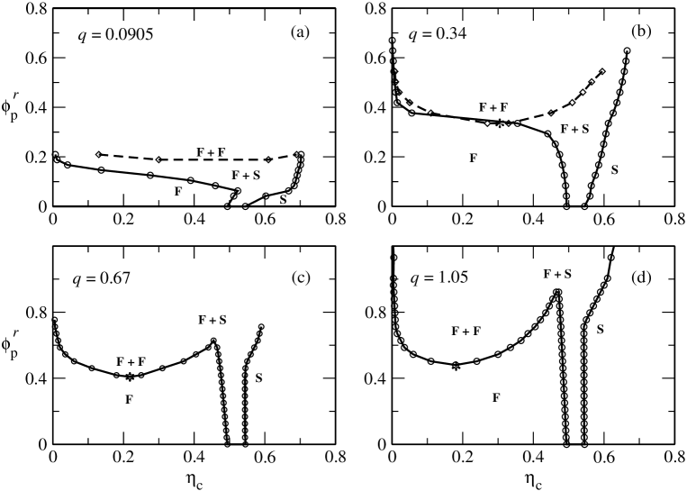
Figure 5: Phase diagrams of colloid / ideal polymer mixtures as obtained from perturbation theory for the effective one-component system using $v_{id}(r)$ (eq. (6)) for the same $q$’s as in figure 4, as functions of the colloid packing fraction $\eta_{c}$ and the polymer concentration $\phi_{p}^{r}$ in the reservoir. Note that the critical points (asterisks) are always at lower $\phi_{p}^{r}$ than the corresponding crtitical points for interacting polymers.

The corresponding phase diagrams for mixtures of colloids and ideal polymers, calculated using the ideal depletion potential (6) are shown figure 5 for comparison. While they look qualitatively similar to those for interacting polymers in figure 4, there are a number of striking quantitative differences. Because the depletion attraction for ideal polymers (eq. 6) is stronger than that for interacting polymers (eq. (2)) for the same polymer concentration, the fluid-fluid phase separation becomes stable at a larger $\phi_{p}^{r}$ for the interacting than for the non-interacting polymers. While the phase diagrams for $q\simeq 0.1$ are fairly close, the differences grow with increasing $q$. For $q\simeq 1$ the critical point in figure 5 (ideal case) is at ($\eta_{c}=0.18$,$\phi_{p}^{r}=0.48$) compared to (0.25,1.21) in the interacting case, while the triple points are at (0.47,0.92) and (0.43,1.42) respectively, indicating dramatic changes when going from ideal to interacting polymers. Also note that while the critical polymer concentration is practically independent of $q$ (for $q\gtrsim 0.35$) in the ideal case, it shifts to higher values as $q$ increases in the interacting case. On the other hand, the critical colloid packing fraction decreases as $q$ increases in the non-interacting case, while it is practically constant for interacting polymers.

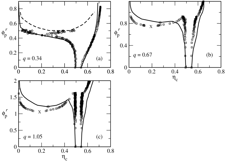
Figure 6: Phase diagrams of colloid / interacting polymer mixtures, as obtained from perturbation theory for the effective one-component system (lines), compared to simulations of the two-component system (symbols) PRL89 . The size ratios are (a) $q=0.34$, (b) $0.67$ and (c) $1.05$. The critical points are indicated by crosses (two-component) and asterisks (one-component). The agreement is surprisingly good.

All these trends are similar to those reported recently in simulations of the two-component description of mixtures of colloids and SAW polymers PRL89 . A detailed comparison between the present perturbation theory results for the effective one-component system, and the phase diagrams determined for the two-component representation is made in figure 6. The agreement between the simulation data for the two-component representation and the predictions of perturbation theory for the effective one-component representation is seen to be reasonable, but not perfect, and to deteriorate as $q$ increases. The obvious reason is that perturbation theory only includes the pair-wise additive part of the depletion interactions, while the two-component representation also accounts for effective many-body depletion interactions between colloidal particles. The fact that the phase diagrams obtained from the two-component representation are shifted to lower polymer concentrations relative to the prediction for the effective one-component system indicates that the more-than-two-body depletion interactions are overall attractive in nature. The opposite trend was found in the case of ideal polymers dijkstra , and is consistent with the more pronounced trends in the limit of large $q$ long-pol .

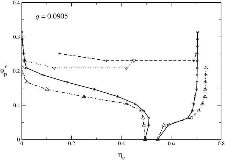
Figure 7: Phase diagram for colloid / interacting polymer mixture, as a function of the colloid packing fraction $\eta_{c}$ and the polymer concentration $\phi_{p}^{r}$ in the reservoir, for a small size ratio ($q=0.0905$). The solid (resp. dashed-dotted) line denotes the fluid-solid binodal obtained from perturbation theory (resp. from MC simulations of the effective one-component system), while the dashed (resp. dotted) line denotes the metastable fluid-fluid binodal obtained by the same methods.

We pointed out earlier that the convergence of thermodynamic perturbation theory is expected to deteriorate when the range of the attractive potential well decreases, i.e. when $q$ decreases. To check the reliability of second order perturbation theory at $q\simeq 0.1$, we have systematically computed the “exact” free energy by MC simulations, using the $\lambda$-integration (eq. (11)). The phase diagrams determined with the approximate and “exact” free energies are compared in figure 7. The agreement remains acceptable for the fluid-solid transition, even for $q\simeq 0.1$, but the (metastable) critical point of the fluid-fluid transition is at too high a colloid packing fractiondijkstra .

Two-component simulationsPRL89 would be very expensive for small $q$, because the number of polymers needed scales as $q^{-3}$. However, for sufficiently small $q$ we don’t expect many-body interactions to be important, and so our one-component simulation should accurately represent the true colloid / polymer system.

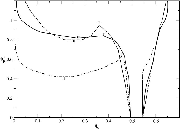
Figure 8: Phase diagrams of colloids/polymer mixtures within three different one-component models: ideal polymers (dashed-dotted lines, $R_{g}=0.67$), interacting polymers (solid lines, $R_{g}=0.67$) and star polymers with functionality $f=2$ (dashed lines, $R_{g}=0.6$). The critical points are indicated by asterisks, while the symbol $T$ denotes the triple points.

A final instructive comparison is between the present results for the phase behaviour of colloid/interacting polymer mixtures and the results for colloid/star polymer mixtures of functionality $f=2$dzubiella , which reduce in fact to interacting linear polymers considered in the present work. The phase diagrams calculated from both depletion potentials within the same approximation (10) for the free energies are compared in figure 8 for similar size ratios $q$. Although, as explained earlier in this paper, the depletion pair potential calculated for the $f=2$ star polymers dzubiella is not quite the same as the more accurate one we useJCP117 , the phase-diagrams show the similar trends when compared to ideal polymers.

V Conclusion

We have shown that traditional thermodynamic perturbation theory, requiring only the well-documented equations of state and pair distribution functions of the fluid and solid phases of the reference hard sphere system, leads to reasonably accurate phase diagrams of mixtures of colloidal particles and interacting polymer coils, provided the appropriate concentration-dependent depletion potential between two colloidal spheres is used. As expected, the agreement between the predictions of the effective one-component description, and the more elaborate two-component description observed for low size ratios $q$ deteriorates as $q$ increases, due to the enhanced importance of many-body interaction which are neglected in the one-component picture. Nevertheless, the disagreement remains tolerable even at $q\approx 1$, and in view of the excellent agreement between the predictions of the two-component description PRL89 and recent experimental data ilett ; ramak , we conclude that the effective one-component picture, in conjunction with standard thermodynamic perturbation theory, provides a reliable prediction of the phase diagrams of colloids/polymer mixtures in good solvent.

A direct comparison between the phase diagrams for interacting and ideal polymers calculated at the same level of approximation shows considerable quantitative, and even qualitative differences between the two depletants. The main effect of polymer-polymer interactions is to enhance the miscibility of the colloid / polymer mixtures. Similar conclusions were reached by a number of different recent investigations, based on two-component approaches, including integral equationsfuchs , “polymers as soft colloids”PRL89 , extensions of free-volume theoryaarts , density functional theoryschmidt , and star-polymer potentialsdzubiella . Here we show that the differences between the two types of depletants can be rationalised within a one-component effective potential picture, mainly because for a given $R_{g}$ and density $\rho_{p}$, the depletion potentials for interaction polymers are less attractive than those for interacting polymers.

The results of the present work apply to polymers in good solvent, for which the SAW model constitutes an excellent representation. We plan to examine the situation where solvent quality is such that attractive forces between monomers can no longer be neglected krakovi . Upon lowering the temperature from very high (corresponding to the SAW limit) to the $\theta$ temperature, we should be able to investigate the gradual change in the phase diagrams from the fully interacting case to one similar to the ideal polymer limit, which have both been considered in the present paper.

			Perturbations		Simulations
$\phi_{p}^{r}$	$\eta_{c}$	State	$\widetilde{F}_{1}^{pert}$	$\widetilde{F}_{2}^{pert}$	$\widetilde{F}_{1}^{MC}$	$\widetilde{F}_{2}^{MC}$
0.17	0.22	Fluid	-0.194	-0.004	-0.193	-0.006
	0.64	Solid	-2.692	-0.001	-2.701	-0.032
0.29	0.22	Fluid	-0.318	-0.012	-0.318	-0.021
	0.64	Solid	-4.663	-0.003	-4.679	-0.097
0.42	0.22	Fluid	-0.434	-0.025	-0.433	-0.043
	0.64	Solid	-6.900	-0.006	-6.941	-0.210
0.54	0.22	Fluid	-0.535	-0.041	-0.534	-0.077
	0.64	Solid	-8.604	-0.011	-8.635	-0.329

Table 1: First two terms of the perturbation series, as obtained using equation (10) ($F^{pert}$), and by MC simulations ($F^{MC}$), for several colloid and polymer concentrations, and for $q=0.67$. The free energy densities are given in reduced units $\widetilde{F}=\beta F(2R_{c})^{3}/V$. Whereas both $F_{1}^{pert}$ and $F_{2}^{pert}$ are accurate in the fluid phase, the latter underestimates the absolute value of $F_{2}^{MC}$ in the solid phase.

			$\widetilde{F}_{0}+\widetilde{F}_{1}+\widetilde{F}_{2}$		$\widetilde{F}$
$\phi_{p}^{r}$	$\eta_{c}$	State	Perturbations	Simulations	$\lambda$-integration
0.17	0.22	Fluid	-0.055	-0.056	-0.056
	0.64	Solid	7.551	7.511	7.541
0.29	0.22	Fluid	-0.194	-0.196	-0.196
	0.64	Solid	5.578	5.468	5.562
0.42	0.22	Fluid	-0.316	-0.333	-0.339
	0.64	Solid	3.582	3.368	3.563
0.54	0.22	Fluid	-0.434	-0.468	-0.483
	0.64	Solid	1.629	1.279	1.605

Table 2: Truncated free energy densities $F_{0}+F_{1}+F_{2}$, in reduced units (see table I), as obtained using equation (10) and MC simulation, and total free energy of the system, as obtained from $\lambda$-integration (equation (11)). Whereas the results of MC simulations are accurate only in the fluid phase, thoses obtained using equation (10) are in good agreement with $\lambda$-integration in both phases.

Figure 3: Ratio of the first two perturbative terms $F_{2}/F_{1}$, as a function of the colloid packing fraction $\eta_{c}$ and the polymer density in the reservoir $\phi_{p}^{r}$. The diamonds are for the fluid phase and the crosses ($\eta_{c}\geq 0.5$) for the solid phase. The size ratio is $q=0.67$.