Resonances in 1D disordered systems:
localization of energy and resonant transmission

Abstract

Localized states in one-dimensional open disordered systems and their connection to the internal structure of random samples have been studied. It is shown that the localization of energy and anomalously high transmission associated with these states are due to the existence inside the sample of a transparent (for a given resonant frequency) segment with the minimal size of order of the localization length. A mapping of the stochastic scattering problem in hand onto a deterministic quantum problem is developed. It is shown that there is no one-to-one correspondence between the localization and high transparency: only small part of localized modes provides the transmission coefficient close to one. The maximal transmission is provided by the modes that are localized in the center, while the highest energy concentration takes place in cavities shifted towards the input. An algorithm is proposed to estimate the position of an effective resonant cavity and its pumping rate by measuring the resonant transmission coefficient. The validity of the analytical results have been checked by extensive numerical simulations and wavelet analysis.

I Introduction

Localization of waves in random media has been investigated intensively during last few decades. One-dimensional (1D) strong localization has received the most study, both analytically and numerically. Localization of eigen states in closed 1D disordered systems and exponentially small (with respect to the length) transparency of open systems with 1D disorder have been studied with mathematical rigor (see, for example, Ref. 1 and references therein). The most common physical manifestation of these effects is the fact that a thick stack of transparencies reflects light as a rather good mirror.berry Much less evident (though also well known theoretically) is that for each (sufficiently long ) disordered 1D sample, there exists a quasi-discrete set of frequencies that travel through the sample unreflected, i.e. with the transmission coefficient close to one.^3-5 Values of these frequencies are random, determined exclusively by the structure of the realization, and the whole set of frequencies constitutes a fingerprint of a given random sample.

High transparency is always accompanied by a large concentration (localization) of energy in randomly arranged points inside the system. Therefore, an open random 1D sample can be considered as a resonator with a set of modes (resonances) with high quality factors. An important feature of such systems is that, in distinction to a regular resonator whose modes occupy all inner space, in a 1D random sample each mode (frequency) is localized inside its own effective ’cavity’ whose position is random and size is much smaller than the size of the sample. The resonances are sharp and well pronounced in the sense that their widths are much smaller than the distances between them, both in the frequency domain and in real space. Therefore, it is of little wonder that resonances caused by one-dimensional disorder have recently attracted considerable interest of physicists looking for the possibility of creating random laser.^6-10

In this paper, we investigate the localized states (modes, or resonances) in one-dimensional open random systems. To understand the nature of the resonances in disordered 1D systems and to describe them quantitatively, the problem is mapped onto a quantum mechanical problem of tunnelling and resonant transmission through an effective two-humped regular potential. With the formulas derived on the basis of this mapping, we find statistical characteristics of the resonances, namely, their spectral density, spectral and spatial widths, as well as the amplitudes of the field peaks and transmission coefficient. Based on these results, one can solve an inverse problem, namely, to predict (with some probability) for each resonance the position of the effective cavity and the maximal pumping amplitude, using the total length of the sample and localization length as the fitting parameters, and the transmission coefficient as the only (measurable) input datum. The analytical results deduced from the quantum-mechanical analogy are in close agreement with the results of numerical experiments.

We study the frequency dependence of the transmission coefficient and the spatial intensity distribution induced by incident monochromatic waves with different frequencies. If the frequency of the incident wave coincides with one of the ’eigen frequencies’ of the sample, the energy is genuinely localized in some randomly located area of the size of the localization length. Thus, the transparency of this area is abnormally high, whereas the transparency of the adjacent segments is exponentially small. The transparent segment surrounded by non-transparent parts of the sample constitutes an effective resonant cavity with a high Q-factor. The transmission coefficient at a resonance is independent of the total length, $L$, of the sample and is determined only by the location of the cavity, that is, totally different from the typical transmission that decays exponentially with increasing $L$ . The maximal transmission is provided by the modes that are located in the center, while the highest energy concentration takes place in cavities shifted towards the input. The number of the resonantly transparent frequencies is shown to be $L/l_{loc}\gg 1$ times smaller than the total number of resonances ($l_{loc}$ is the localization length). Wavelet analysis of random realizations supports the validity of the mapping and provides physical insight into the origin of the effective cavities in disordered samples.

II Formulation of the problem

We consider a plane monochromatic wave with wavelength $\lambda$ and unite amplitude incident from the left ($x<0$) on a 1D disordered sample with randomly fluctuating refractive index. The transmission coefficient, $T(\lambda)$ and the random field amplitude, $A=|E(x)|$, have been studied both analytically and numerically. Typical frequency dependence of the transmission coefficient of a 1D randomly layered sample is shown in Fig.1.

One can see that along with a continuum of wavelengths for which the transmission coefficient is exponentially small ($\sim\exp(-2L/l_{loc})$), there is a discrete set of points at $\lambda$-axis ($\lambda_{b},\lambda_{c}$ in Fig.1) where $T(\lambda)$ has well pronounced narrow maxima. The amplitude distributions induced by the corresponding waves inside the sample are shown in Fig.2. While at typical frequencies (realizations) the amplitude of the field decrees exponentially from the input (Fig. 2, $\lambda_{a}$), the resonances, (Fig. 2, $\lambda_{b,}$ $\lambda_{c}$), exhibit essentially non-monotonous spatial distribution of the amplitude.

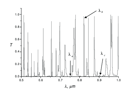
Figure 1: Transmission coefficient as a function of the wavelength.

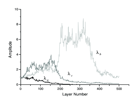
Figure 2: Amplitude of the field inside the sample as a function of the coordinate for three wavelengths marked in Fig. 1.

Important to note that the localization of energy takes place for all resonances, not only for those with the transmission coefficient close to one (Fig. 2, $\lambda_{b,}$ $\lambda_{c}$). The amplitude of a maximum depends on its location in space, which in its turn, is uniquely determined by the internal structure of the realization. As it is shown below, this fact provides a means for evaluating the resonant amplitude and the coordinate of the point where the resonant mode is localized, if the total transmission coefficient is known.

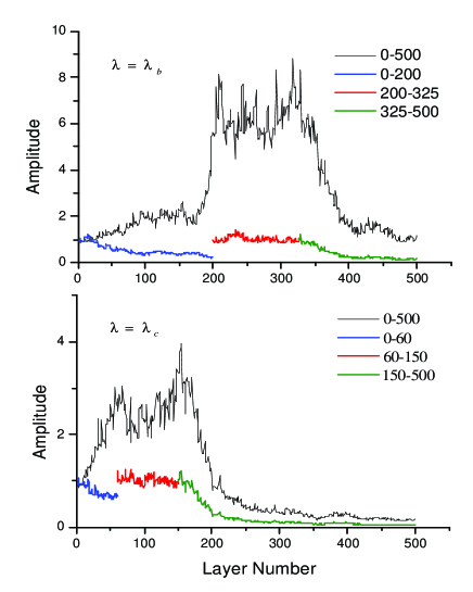
Figure 3: Amplitude of the field as a function of the coordinate inside the whole sample (black curves), in the left (blue curves), middle (red curves), and right (green curves) parts taken as a separate sample each. $\lambda=\lambda_{b}$ and $\lambda=$ $\lambda_{c}$.

Fig. 3 demonstrates the connection between the amplitude distribution and the transparency of different parts of the sample. The upper picture shows the intensities of the field generated by a resonantly transmitted wave with $T\simeq 1$ ($\lambda_{b}$ in Fig. 1) inside the whole sample (black curve), and in their left (blue curve), middle (red curve), and right (green curve) parts when they are taken as a separate sample each. The same dependencies for resonant wave with $T<1$ ($\lambda_{c}$ in Fig. 1) are depicted in the lower picture. It is seen that the middle sections where the energy is concentrated are almost transparent for the wave, while the side parts are practically opaque for the resonant frequencies. Wavelet analysis of the power spectra of the transparent and non-transparent parts presented in Sec. 6 provides physical insight into their nature.

Structures of this type have been studied in the quantum mechanical problem of the tunnelling and resonant transmission of particles trough a regular (non random) potential profile consisted of a well bounded at both sides by two potential barriers (Fig. 4) bohm . Although the physics of the propagation in each system is totally different (interference of the multiply scattered random fields in a randomly layered medium, and tunnelling through a regular two-humped potential), the similarity of this two problems turns out to be rather close. Indeed, in both cases the transmission coefficients are exponentially small for most of frequencies (energies), and have well-pronounced resonant maxima (sometimes of order of unity) at discrete points corresponding to the eigen levels of each system. The energy at resonant frequencies is localized in a transparent part, and the total transmission depends drastically on the position of this part. More than that, even qualitatively the intensity distributions presented in Fig. 3 and the corresponding values of the transmission coefficients compare favorably with those calculated for a potential profile depicted in Fig. 4 if the parameters of the effective profile have been chosen properly.

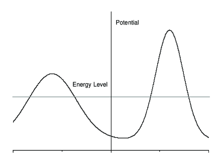
Figure 4: Two-humped potential profile.

III Quantum mechanical formulas

To map the stochastic classical wave scattering problem in hand onto a deterministic quantum mechanical one, that is to say, to construct an appropriate effective regular potential that provides the same transmission and the interior intensity distribution, let us consider an auxiliary problem of the transmission of a quantum particle through a potential profile (resonator) consisted of two barriers separated by a potential well (Fig. 4). The transmission coefficient through the potential can be calculated in WKB approximation bohm , which yields

$$T=\left[\left(\frac{\Theta_{1}^{2}+\Theta_{2}^{2}}{2\Theta_{1}\Theta_{2}}\right)\cos^{2}\frac{1}{2}(\pi-J)+\frac{1}{4}\left(4\Theta_{1}\Theta_{2}+\frac{1}{4\Theta_{1}\Theta_{2}}\right)^{2}\sin^{2}\frac{1}{2}(\pi-J)\right]^{-1}~{}.$$ (1)

Here $\Theta_{i}=T_{i}^{-1/2}\gg 1$ with $T_{i}$ being the tunnelling transmission coefficients of the barriers, $J/2$ is the phase acquired in the well,

$$J=2\int_{l_{0}}k(x)dx\sim 2kl_{0}~{},$$ (2)

$k(x)$ is the momentum ($\hbar=1$), and $l_{0}$ is the length of the well. At $\Theta_{1}=\Theta_{2}\equiv\Theta$ (symmetrical potential) equation (1) transforms into

$$T=\left[1+\frac{1}{4}\left(4\Theta^{2}-\frac{1}{4\Theta^{2}}\right)^{2}\sin^{2}\frac{1}{2}(\pi-J)\right]^{-1}~{}.$$ (3)

Since $\Theta_{i}^{2}\gg 1$, it follows from Eqs. (1), (3) that typically $T\ll 1$. Resonance transmission ($T\simeq 1$) takes place only at the discrete points that correspond to the eigen levels of the well:

$$J=\pi\left(n+\frac{1}{2}\right)~{},~{}~{}n=0,1,2,...~{}.$$ (4)

Thus, the characteristic spectral interval between the resonances is determined by the requirement $\Delta J=\pi$, or

$$\Delta k_{res}\sim\frac{1}{l_{0}}~{}.$$ (5)

To estimate the half-width of the resonances, $\delta k$, we note that in the vicinity of $k_{res}$ the transmission coefficient Eq. (3) takes the form

$$T\simeq\frac{1}{1+4l_{0}^{2}\left(k-k_{res}\right)^{2}\Theta^{4}}$$ (6)

(with $T_{res}=1$), from which it follows that

$$\delta k\simeq\frac{1}{2l_{0}\Theta^{2}}~{}.$$ (7)

In general (asymmetrical) case Eq. (1) the transmission coefficient at a resonance is equal

$$T_{res}=\left(\frac{2\Theta_{1}\Theta_{2}}{\Theta_{1}^{2}+\Theta_{2}^{2}}\right)^{2}~{}.$$ (8)

It is easy to see that asymmetry of the potential profile reduces drastically the resonance transmission: $T_{res}\ll 1$ if $\Theta_{1}^{2}\ll$ $\Theta_{2}^{2}$ or $\Theta_{1}^{2}\gg\Theta_{2}^{2}$. In the same approximation the amplitude of the wave function in the well is given by

$$|A|\simeq\frac{2\sqrt{2}\Theta_{1}\Theta_{2}^{2}}{\Theta_{1}^{2}+\Theta_{2}^{2}}.$$ (9)

IV Application to the resonances in disordered systems

To use the above-derived formulas for the qualitative description of the wave transmission through a random sample we have to express the parameters of the effective potential through the statistical parameters of the disordered system in hand. For an ensemble of 1D random realizations those parameters are the total length $L$ and the localization length $l_{loc}$ that we define as $l_{loc}=2L/<\ln T^{-1}>^{-1}$. Note that in the localized regime $L\gg l_{loc}\gg\lambda$. This inequality justifies the validity of WKB approximation. To determine properly the length of the (effective) well in disordered systems we note that the appearance of a transparent segment (effective well) inside a random sample is the result of a very specific (and therefore low-probable) combination of phase relations. Obviously, the longer such segment is, the less is the probability of its occurrence. On the other hand, the typical scale in the localized regime is $l_{loc}$. Hence, the minimal and, therefore, the most probable size of the effective well is $l_{0}\sim l_{loc}$ that we assume to be the same in all realizations. Under this assumption, different values of the resonant transmission coefficients and different intensity distributions at different resonant realizations can be reproduced by variations of the location of the well in the corresponding quantum formulas presented in Sec. 3 with

$$l_{0}=l_{loc}~{}.$$ (10)

If the center of the transparent segment of a resonant realization is shifted on the distance $d$ from the center of the sample, the lengths of the non-transparent parts of resonant realizations are

$$l_{1,2}=\frac{L-l_{loc}}{2}\pm d~{},$$ (11)

with transmission coefficients $T_{i}=\exp\left(-2l_{i}/l_{loc}\right)$. Therefore functions $\Theta_{i}$ in Eqs. (1)-(9) should be taken in the form

$$\Theta_{1,2}=\exp\left(\frac{l_{1,2}}{l_{loc}}\right)=\exp\left(\frac{L-l_{loc}}{2l_{loc}}\pm\frac{d}{l_{loc}}\right)~{}.$$ (12)

The above-introduced mapping, Eqs. (10)-(12), allows the use of Eqs.(1)-(9) for evaluating the corresponding quantities related to random 1D systems. It becomes apparent, for example, that not all eigen modes of along random sample provide high transmission ($T\simeq 1$) through the system. Indeed, while the distance (in $k$-space) between eigen modes is

$$\Delta k\sim\frac{1}{L}~{},$$ (13)

the typical interval between the resonantly transparent frequencies obtained from Eq. (5) by substituting Eq. (10) is of order

$$\Delta k_{res}\sim\frac{1}{l_{loc}}~{}.$$ (14)

It is easy to see that $\Delta k/\Delta k_{res}\sim l_{loc}/L\ll 1$, which means that the resonances with $T\sim 1$ occur much less frequently than all other resonances, $T<1$. It is physically clear, and follows from the fact that a resonance with high transmission occurs when the transparent segment is located in the middle of the sample (with accuracy of $l_{loc}$), while the resonances with smaller transmission are observed in any non-symmetrical potentials with arbitrary situated transparent segment. Assuming that the transparent segment can be found at any point of the sample with equal probability, we infer that resonances with $T\sim 1$ are encountered $L/l_{loc}$ times more rarely than all other ones.

It follows from Eq. (7) that typical width of resonances is

$$\delta k\sim\frac{1}{l_{loc}}\exp\left(-\frac{L}{l_{loc}}\right)~{},$$ (15)

that is to say, it decreases exponentially with the length of the sample.

In the same manner, the resonant transmission coefficient at resonant frequencies and peak amplitudes can be estimated from Eqs. (8) and (9),which after substituting Eq. (12) yield:

$$T_{res}(d)=\frac{4}{\exp(2d/l_{loc})+\exp(-2d/l_{loc})}~{},$$ (16)

$$|A(d)|^{2}=\frac{8\exp(L/l_{loc}-1-2d/l_{loc})}{\left[\exp(2d/l_{loc})+\exp(-2d/l_{loc})\right]^{2}}.$$ (17)

Eq. (16) shows that the resonant transmission coefficients do not depend on the total length of the sample and are governed only by the positions of the areas of localization, in contrast to the typical transmission which decays exponentially with $L$ increasing.

If $T_{res}\simeq 1$, then $d\simeq 0$, and Eq. (17) gives

$$|A|\simeq\sqrt{2}\exp\left(L/2l_{loc}\right)\gg 1~{}.$$ (18)

When the transparent segment of a random realization is shifted from the center, it follows from Eq. (17) that

$$|A|\simeq\left[\begin{array}[]{cl}2\sqrt{2}\exp(l_{1}/l_{loc})\gg 1,&\text{if}~{}\exp(l_{1}/l_{loc})\ll\exp(l_{2}/l_{loc})\\ 2\sqrt{2}\exp\left((2l_{2}-l_{1})/l_{loc}\right)\gg 1,&\text{if}~{}\exp(2l_{2}/l_{loc})\gg\exp(l_{1}/l_{loc})l_{1}\gg\exp(l_{2}/l_{loc})\\ 2\sqrt{2}\exp\left((2l_{2}-l_{1})/l_{loc}\right)\ll 1,&\text{if}~{}\exp(l_{1}/l_{loc})\gg\exp(2l_{2}/l_{loc})\end{array}\right.$$ (19)

with $l_{1,2}$ defined in (11).

It can be shown from Eq. (17) that the maximum of the amplitude is reached when the transparent part is shifted from the center of the sample towards the input on the distance

$$d=-\frac{1}{4}\ln\frac{1}{3}~{}l_{loc}\simeq-0.27l_{loc}~{}.$$ (20)

This shift is independent of the length of the sample.

V Numerical simulations

To test the validity of the above-introduced analytical results, Eqs. (13)-(20), numerical calculations of the spectrum of resonances and of the spatial intensity distributions at resonant frequencies have been performed for more than $10^{4}$ resonances. In the calculations we consider samples with up to $N=1000$ of layers, and assume that the refractive indexes and sizes of the layers are independent random variables uniformly distributed in the ranges $n=1\pm 0.25$ and $d=0.15\pm 0.05~{}\mu m$ respectively. The wavelength varies in the interval $0.5\mu m\leq\lambda\leq 1.5\mu m$.

In accordance with Eq. (14) the average spacing between resonantly transparent modes with $T\simeq 1$ depicted in Fig. 5 (curve b) is determined by the localization length and practically independent on the size $L$ of the system. For comparison, the numerically calculated $L$-dependence of the eigen mode spacing is also shown in Fig. 5 (curve a). It fits well Eq. (13). Numerically calculated average half-width of the resonances (Fig. 6) is consistent with the analytical expression Eq. (15). The localization length had been computed through the transmission coefficient as $l_{loc}=-2L<\ln T>.$ Note that, being a self-averaging quantity lif , $l_{loc}$ slightly fluctuates from sample to sample, and can be estimated from the transmission coefficient at a typical realization.

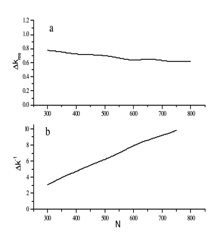
Figure 5: Inverse spacing between eigen modes, (a), and spacing between resonantly transparent eigen modes, $T\simeq 1,$ (b), as functions of the length of the sample.

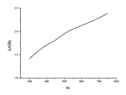
Figure 6: Logarithm of the half-width of the resonances as a function of the length of the sample.

Depicted in Fig. 7 is the probability that a mode localized at a given point provides transmission coefficient $T$ (dimensionless coordinate $x/L$ is used). As is seen from the picture, the probability of high transitivity ($T\simeq 1$) has maximum for modes that are localized in the center of the random sample. As the location of an effective cavity shifts from the center, the corresponding transmission coefficient decreases, in agreement with Eq. (16). To make the comparison with the analytical results more convenient, the same (as in Fig. 7) probability density distribution is presented in Fig. 8 as a two-dimensional picture where different colors correspond to different probabilities. Black line displays the transmission coefficient calculated by Eq. (16) as a function of the coordinate of the corresponding point of localization. Note that shifted to the exit peaks of the field are not shown in Fig. 8. They are much weaker, because they happen on the background of an exponentially small signal.

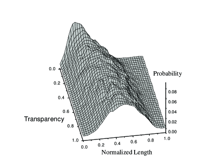
Figure 7: Probability for a mode localized at a given point to provide the value of the transmission coefficient $T$ , as a function of the dimensionless coordinate $x/L.$

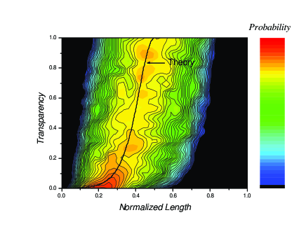
Figure 8: The same probability as in Fig. 7 presented by colors. Black line displays the transmission coefficient as a function of the coordinate of the point of localization calculated by Eq. (16).

Numerically calculated average normalized field amplitude of localized modes (pumping rate of effective resonant cavities) as a function of the coordinate of the cavity exponentially increases with the length of the sample in a good agreement with Eq. (17). Effective cavities which provide the highest pumping rate are shifted from the center towards the input in accordance with Eq. (20). Interestingly enough, the seemingly rough analogy based on only one fitting parameter (localization length) performs surprisingly well. Indeed, not only the shift is independent on the total length and proportional to $l_{loc}$ as predicted by Eq. (20), but also the coefficient in Eq. (20) coincides with that obtained in numerical simulations with the accuracy 10%. We have also verified that the maximal peak amplitudes exponentially increase with the length of a sample and by the order of magnitude coincide with the values given by Eqs. (18).

VI Wavelet analysis of random samples

Here we discuss briefly why the effective resonant cavities exist in 1D disordered samples, in other words, why different segments of a random sample are transparent or non-transparent for the wave with given wave number $k={2\pi}/{\lambda}$. It is well known that in the case of a weak scattering the so called resonance reflection takes place, that is, the reflection coefficient (and, therefore, the transparency) of some segment of a random medium is determined by the amplitude of the resonance harmonic with $q_{res}=2k$ in the spatial Fourier transformation of its refractive index ryt . In other words, any long enough randomly layered segment, $x_{1}<x<x_{2},$ resonantly reflects as a periodically modulated medium whose modulation wave number $q$ is determined by the resonance condition $q=q_{res}=2k,$ and the amplitude, $\widetilde{n}^{2}(q_{res})$, is

$$\widetilde{n}^{2}(q_{res})=\int_{x_{1}}^{x_{2}}n^{2}(x)e^{-i2kx}dx~{}.$$ (21)

This expression is known as window Fourier transform with the rectangular window function, and characterizes the local spectrum of the investigated function. The rectangular window function has some disadvantages that disappear when instead of the window Fourier transform, a wavelet transform is applied for the determination of the local spatial spectrum of the sample. To investigate the local spectra of different parts of the sample we used the so-called complex-valued Morlet wavelet morlet . We first have found the wavelengths for which the transparency $T(\lambda)$ of the whole sample exceeds 0.5. For these wavelengths the spatial distributions of the wave amplitude and of the amplitude of the corresponding wavelet transformation have been compared. The examples are shown in Fig. 9. One can see that in the areas where field is localized, i. e. in those that should be transparent for the given frequency, the wavelet amplitude is strongly suppressed, while in the non-transparent parts it has well pronounced maxima. Therefore, in accordance with the resonant scattering mechanism, the resonant cavity for a frequency $\omega$ arises in that area of a disordered sample, where for some reason or other, the harmonic with the wave number $q_{res}=2k$ in the power spectrum of the (random) refractive index has small amplitude. In a sense the wavelet amplitude can be interpreted as an effective potential. Note, not all resonance realizations exhibit so good correlation with the wavelet analysis as shown in Fig. 9. Actually the correlation was observed for 70 - 80 % of all resonances.

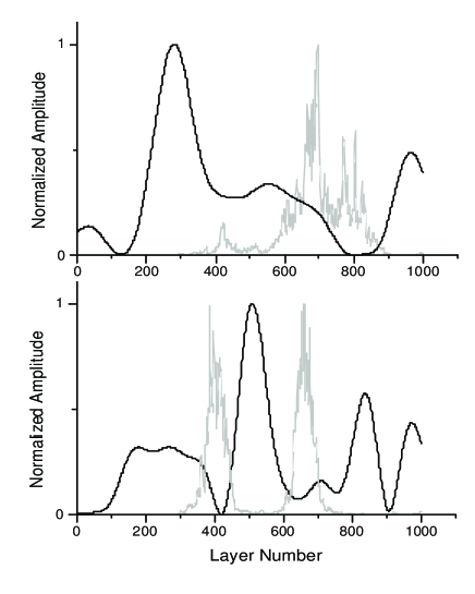
Figure 9: Field amplitudes (light lines) and wavelet transformations (dark lines) as functions of the coordinate in two random realizations.

VII Conclusions

From the results above it follows that the resonant transmission through a disordered 1D system occurs due to the existence inside the system of a transparent (for a given resonant frequency) segment with the size of order of the localization length. The mode structure of the sample, the transmission coefficient, and the intensity distribution at resonant frequencies depend on the positions of the segment. These dependencies are very robust, insensitive to the fine structure of the system, and therefore can be described by corresponding formulas for an effective regular potential profile. The fitting parameters are the total length of the sample and the localization length, which is a self-averaging quantity and can be found, for example, from the transmission coefficient at typical (non-resonant) realizations. This feature enables to estimate the position of an effective resonant cavity by measuring the transmission coefficient at a typical and at the corresponding resonant frequencies. From the first data the localization length can be obtained, the second one, $T_{res}$, could be used to find the asymmetry parameter $d$ (i.e. the coordinate of the effective cavity) from Eq. (16).Then Eq. (17) gives estimation for the pumped intensity. Therefore, although locally for 1D photons there is no analog to the quantum mechanical tunnelling (by definition the effective energy of 1D photons is always higher than the effective potential barrier), macroscopically (on scales larger than the localization length) the problem of the propagation of light through a disordered 1D system can be reformulated in terms of the effective potential profile.

References

- (1) I. M. Lifshits, S. A. Gredeskul, and L. A. Pastur, Introduction to the Theory of Disordered Systems (Wiley, New York, 1988).
- (2) M. V. Berry, S. Klein, ”Transparent mirrors: rays, waves and localization”, Eur. J. Phys. 18, 222-228 (1997).
- (3) U. Frisch, C. Froeschle, J.-P. Scheidecker, and P.-L. Sulem, ”Stochastic resonance in one-dimensional random media”, Phys. Rev. A 8, 1416-1421 (1973).
- (4) M. Ya. Azbel, P. Soven, ”Transmission resonances and the localization length in one-dimensional disordered systems”, Phys. Rev. B 27, 831-836, (1983).
- (5) M. Ya. Azbel, ”Eigenstates and properties of random systems in one dimension at zero temperature”, Phys. Rev. B 28, 4106-4125 (1983).
- (6) D. S. Wiersma, ”The smallest random laser ”, Nature 406, 132-133 (2000).
- (7) D. S. Wiersma, S. Cavalieri, ”Light emission: A temperature-tunable random laser ”, Nature 414, 708-709 (2001).
- (8) Xunyia Jiang, C. M. Soucoulis, ”Time Dependent Theory for Random Lazer”, Phys. Rev. Lett. 85, 70-73 (2000).
- (9) H. Cao, Y. G. Zhao, S. T. Ho, E. W. Seelig, Q. H. Wang, and R.P. H. Chang, ”Random Laser Action in Semiconductor Powder”, Phys. Rev. Lett. 82, 2278-2281 (1999).
- (10) H. Cao, Y. Ling, J. Y. Xu, and C. Q. Cao, and P. Kumar, ”Photon Statistics of Random Lasers with Resonant Feedback”, Phys. Rev. Lett. 86, 4524-4527 (2001).
- (11) D. Bohm, Quantum Theory (Prentce-Hall, Inc, New York, 1952).
- (12) S. Rytov, Yu. Kravtsov, and V. Tatarskii, Principles of Statistical Radiophysics v. 4. Wave Propagation Through Random Media (Springer-Verlag, 1989).
- (13) A. Grossman, J. Morlet, ”Decomposition of Hardy function into square integrable wavelets of constant shape”, SIAM J. Math. Anal. 15, 273 (1984).