Kovacs effects in an aging molecular liquid

Abstract

We study by means of molecular dynamics simulations the aging behavior of a molecular model of ortho-terphenyl. We find evidence of a a non-monotonic evolution of the volume during an isothermal-isobaric equilibration process, a phenomenon known in polymeric systems as cross-over (or Kovacs) effect. We characterize this phenomenology in terms of landscape properties, providing evidence that, far from equilibrium, the system explores region of the potential energy landscape distinct from the one explored in thermal equilibrium. We discuss the relevance of our findings for the present understanding of the thermodynamics of the glass state.

If two systems in thermodynamical equilibrium with identical chemical composition have the same temperature $T$ and volume $V$ we immediately know that they experience the same pressure $P$. We know that the two systems will respond in the same way to an external perturbation, and that they will be characterized by the same structural and dynamical properties. The ability to predict the pressure, and the equivalence of structural and dynamical properties, derive from thermodynamical principles.

In the case of glasses, systems in out-of-equilibrium conditions, the $T$ and $V$ values are not sufficient for predicting $P$, since the state of the system depends on its previous thermal and mechanical history. Different glasses, at the same $T$ and $V$, are characterized by different $P$ values. One can ask if the value of $P$ is sufficient to uniquely define the glass state, i.e., if two glasses with identical composition having not only the same $T$ and $V$ but also the same $P$ are the same glass. If this is the case, the two glasses should respond to an external perturbation in the same way and should age with a similar dynamics.

These basic questions are at the hearth of a thermodynamic understanding of the glassy state of matter, and of the possibility of providing a theoretical understanding of out-of-equilibrium systems. Indeed, if by specifying $T$, $V$ and also $P$, we uniquely define the glass state —its structural and dynamical properties— it means that it is possible to develop an out-of-equilibrium thermodynamic formalism davies53 ; speedy94 ; cugliandolo97 ; nieuwenhuizen98 ; franz00 ; mossa02b where the previous history of the system is encoded in one additional parameter. In the interpretation of experimental data, such additional parameter is often chosen as a fictive temperature or pressure, in the attempt to associate the glass to a liquid, frozen from a specific thermodynamic state.

Back in the 60th, Kovacs and co-workers designed an experimental protocol kovacs63 ; mckenna89 ; angell00 (Fig. 1) to generate distinct glasses with different thermal and mechanical histories but with the same $T$, $V$ and $P$ values. Poly-vinyl acetate was equilibrated at high temperature $T_{h}$ and then quenched at low temperature $T_{l}$, where it was allowed to relax isothermally for a waiting time $t_{w}$ insufficient to reach equilibrium. The material was then re-heated to an intermediate temperature $T$, and allowed to relax. The entire experiment was performed at constant pressure $P$. The observed dynamics of the volume relaxation toward equilibrium—in the last step at constant $T$ and $P$— was striking; the volume crosses over the equilibrium value, passes trough a maximum, which depends upon the actual thermal history of the system, and then relaxes to the equilibrium value. The existence of a maximum clearly indicates that there are states with the same $V$ (at the left and at the right of the maximum) which, although $T$, $V$ and $P$ are the same, evolve differently. Thus, this experiment strongly support the idea that three variables are not always sufficient to uniquely predict the state of the glass nota3 .

Here we attempt to reproduce numerically the Kovacs experiment, performing molecular dynamics simulations for a simple molecular model, to develop an intuition on the differences between states with the same $T$,$V$ and $P$ and the conditions under which out-of-equilibrium thermodynamics may be used to describe glass states. We find that for sufficiently deep quenching temperatures, and long aging times, following the protocol proposed by Kovacs, it is indeed possible to identify two distinct states with the same $T$, $V$ and $P$. Thus, for the first time, Kovacs’ effects, also know in the literature as cross-over effects scherer86 , are also observed in a molecular liquid model. Exploiting the possibilities offered by the information encoded in the numerical trajectories, we examine the differences between this pair of states, and contrast them with corresponding equilibrium liquid configurations. We discover that when the system is forced to age following significant $T$-jumps, i.e., low $T_{l}$, it starts to explore regions of the landscape which are never explored in equilibrium. Under these conditions, it is not possible any longer to associate a glass to a ”frozen” liquid configuration via the introduction of a fictive temperature or pressure. This finding limits the range of validity of recent theories for out-of-equilibrium systems, based on the possibility of developing a thermodynamic formalism for glasses introducing only one additional effective parameter in the free energy nieuwenhuizen98 ; cugliandolo97 ; franz00 ; st01 ; mossa02b .

We consider a system of $343$ molecules, interacting via the Lewis and Wahnström potential lewis94 (LW), a model for the fragile glass former ortho-terphenyl (OTP). The molecule is rigid, composed by three sites located at the vertexes of an isosceles triangle. Sites pertaining to different molecules interact by the Lennard-Jones potential. Simulation details are given in Refs. mossa02a ; lanave02 . The system has been studied in isobaric-isothermal conditions; the time constants of both the thermostat and the barostat have been fixed to $20$ $ps$. In order to accumulate an accurate statistics for the analysis below, averages over up to $200$ different starting configurations have been performed. The total simulation time is more than $6$ $\mu s$.

Figure 1: Top: (a) Temperature protocol in Kovacs experiment: in the numerical simulation the system equilibrated at $T_{h}$ is quenched at several $T_{l}$ (1) where it relaxes for a time $t_{w}$ (2). It is finally heated at $T$ (3). (b) Corresponding volume evolution in the cases of low (A) and high (B) $T_{l}$. Bottom: Volume relaxation at different $T_{l}$. The fast relaxation taking place for times shorter than the thermostat characteristic time is not reported.

Figure 2: Volume relaxation showing Kovacs effect in a molecular system. Top: A system of $343$ molecules of the LW OTP at constant pressure $P=16$ MPa is equilibrated at $T_{h}=400K$, quenched at several low temperatures $T_{l}$ and leaved to age for $t_{w}=50$ ns, a time insufficient to reach equilibrium at $T_{l}$. The system is then heated at the intermediate temperature $T=280$ K and the $V$ relaxation dynamics is recorded (symbols). For the case $T_{l}=T$, the system is directly brought from $T_{h}=400K$ to $T=280K$ and hence $t_{w}=0$. The vertical dashed lines indicate the transient time, where $T$ and $P$ have not yet equilibrated to the final values. Bottom: Volume relaxation at $T=280$ K, at fixed $T_{l}=150$ K for different $t_{w}$ values. Dashed lines delimitate the transient region, when neither $T$ nor $P$ have reached their equilibrium value.

To reproduce the Kovacs experiment, equilibrium configurations at $T_{h}=400\;K$, volume per molecule $V=0.378$ nm³ and $P=16$ MPa are isobarically quenched at several low temperatures $T_{l}$, and left to age for different $t_{w}$ values ($t_{w}$ is never sufficient to reach equilibrium at $T_{l}$). Each resulting configuration is then isobarically heated to $T=280$ K (see Fig. 1). At $T$ the characteristic structural relaxation time is of the order of a few $ns$, allowing us to follow, with the present computational resources, the dynamics up to equilibrium. The $V$-evolution is recorded along the entire path. We also perform an analysis of the properties of the explored potential energy landscape (PEL) as a function of time, focusing in particular on the energy $e_{IS}$ and pressure $P_{IS}$ of the closest local minima configurations (the inherent structures, $IS$), as well as the average curvatures of the PEL around the $IS$ configurations. The $IS$ configuration, which is numerically evaluated performing a steepest descent path along the potential energy surface, can be though of as the low-$T$ glass generated by instantaneously freezing the liquid.

Fig. 2(a) shows the time evolution of $V$ at constant $T=280$ K and $P=16$ MPa for samples which have previously aged at different $T_{l}$ for $t_{w}=50$ ns. The time evolution of $V$ for the case $T_{l}=T$ (i.e. for a $T$-jump from $T_{h}$ to $T$) is also reported. We note that for large $T_{l}$ (i.e., $T_{l}=220$ K), $V$ relaxes to the equilibrium value from below monotonically. Similarly, for $T_{l}=T$, $V$ relaxes to the equilibrium value from above, again monotonically. At variance, for deep $T_{l}$ values, $V$ does not relax monotonically to the equilibrium value. In analogy with Kovacs findings, it goes through a maximum, whose value is higher the lower $T_{l}$, before starting to relax toward the equilibrium value. After the maximum, the time evolution of $V$ practically coincides with case $T_{l}=T$.

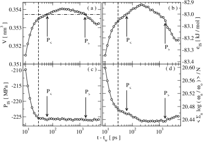
Figure 3: Kovacs effect for $T_{l}=150$ K and $t_{w}=25$ ns; average over $200$ independent realization. The out-of-equilibrium evolution of (a) system volume $V$, (b) inherent structures $e_{IS}$, (c) inherent structure pressure $P_{IS}$, and (d) shape factor ${\cal S}$ are shown. Error bars are smaller than the symbols. Two points (labeled $P_{<}$ and $P_{<}$), characterized by the same values of $T$, $P$, and $V$ are marked by arrows.

The waiting time dependence of $V$ during the final relaxation at $T$ is shown in Fig. 2(b) for the case $T_{l}=150$ K. For all studied $t_{w}$ values, a maximum is observed, and the value of the maximum is larger the shorter the waiting time $t_{w}$. All together, Figs. 2(a) and (b) confirm that the features observed by Kovacs in experiments with polymers are also observable in the case of molecular glass forming liquids under deep-quench conditions (small $T_{l}$ values).

Next we study the properties of the region of the PEL explored by the system during the the aging process. In Fig. 3 we show — for the case $T_{l}=150$ K for which a clear non-monotonic $V$-relaxation is observed — the out-of-equilibrium evolution of (a) the $V$, (b) the average inherent structures energy $e_{IS}$, (c) the average inherent structure pressure $P_{IS}$, and (d) the shape factor ${\cal S}\equiv\sum_{k=1}^{6N-3}\log(\omega_{k}/\omega_{o})/N$ (here the $\omega_{k}$ are the eigenvalues of the Hessian calculated at the inherent structures and $\omega_{o}$ is the frequency unit); the quantity ${\cal S}$ provides a measure of the volume of the basin of attractions) sciortino99 . The maximum in the time evolution of $V$ allows us to define two arbitrary points $P_{<}$ and $P_{>}$ (marked in Fig. 3), characterized, by construction, by the same $T$, $P$, and $V$ values. Although $P_{<}$ and $P_{>}$ are indistinguishable from a thermodynamical point of view, the subsequent dynamics is completely different in the two cases: after $P_{<}$ the system expands, while after $P_{>}$ it contracts. From a landscape point of view, $P_{<}$ and $P_{>}$ differ both in the depth and the shape of the sampled basin. The picture that emerges is that, at $P_{<}$, the system populates local minima which are systematically characterized by energy higher and basins of attraction steeper than the ones explored at $P_{>}$.

Figure 4: Volume dependence of $e_{IS}$(a) ,$P_{IS}$ (b) and ${\cal S}$ (c) during the relaxation dynamics at $T=280K$, for samples which have aged at $T_{l}=150$ K, $220$ K and $280$ K. Only data for times longer than $20~{}ps$ — the time associated to the establishment of constant $T$ and $P$ conditions — are shown. Note that $P_{IS}$ is constant. The solid lines show the equilibrium relation $e_{IS}(V)$, $P_{IS}(V)$ and ${\cal S}(V)$ along a constant $P_{IS}=-225.8$ MPa path. The vertical arrows indicate $P_{<}$ and $P_{>}$ (see Fig. 3).

It is particularly important to note that, after about $20-30$ $ps$, corresponding to the time requested to bring $T$ and $P$ to equilibrium, the $P_{IS}$ value stabilizes, while both depth and shape of the explored basins continues to change with time. This suggests that the vibrational component to the pressure (defined as $P_{vib}=P-P_{IS}$ mossa02b ; lanave03 ) is rather insensitive to the basin properties, in agreement with similar findings from equilibrium studies lanave02 . The fact that $P_{IS}$ is constant offers an unique possibility to estimate how and if the aging dynamics proceeds via a path which is usually explored in equilibrium, by comparing properties in equilibrium along a constant $P_{IS}$ path and the aging dynamics at the same constant $P_{IS}$ value. Indeed, in equilibrium, all landscape properties (i.e., $e_{IS}$, $P_{IS}$, ${\cal S}$) are function only of $T$ and $V$. By eliminating $T$ in favor of $P_{IS}$, $e_{IS}$ can be expressed as a function of $V$ and $P_{IS}$. Therefore, for a fixed value of $P_{IS}$, $e_{IS}$ becomes, in equilibrium, an unique function of $V$. This equilibrium relation can be compared with the same relation along the aging path to estimate which part of the aging dynamics follows the equilibrium properties and which part is instead different from it. A similar comparison can be performed between basin shape ${\cal S}$ and $V$ at constant $P_{IS}$.

This comparison is shown in Fig. 4 for the two cases where a monotonic $V$-relaxation is observed (large $T_{l}$ values, $T_{l}=220$ K and $T_{l}=280$ K), and for the case $T_{l}=150K$ where a maximum in the time evolution of $V$ is clearly detected. The important information standing out from the comparison is that, while equilibration with large $T_{l}$ values follows equilibrium paths, in the other case only the final part of the dynamics follows a path which goes via a sequence of states which are explored in equilibrium. This confirms that only one $(P_{>})$ of the two states with the same $T$, $P$, and $V$ can be related, for example via a fictive temperature expl , to an equilibrium state, while the other one $(P_{<})$ has a structure which is never explored in equilibrium. Therefore the two states, although having the same $T$, $P$, and $V$, are quantitatively different. In other words, while at $P_{>}$ the system samples landscape properties which are sampled by the liquid at equilibrium at a higher temperature (which can be used as additional parameter to quantify the glass properties), at $P_{<}$ the system explores a region of the landscape which is never explored in equilibrium, since the relation between the landscape properties characterizing $P_{<}$ are never encountered in equilibrium. Under these conditions, it is not possible to exactly relate the glass structure to an equilibrium structure and hence define a fictive temperature for the system.

The present numerical study shows that, only when the change of external parameters is small, or when the system is close to equilibrium, the evolution of the equilibrating system proceeds along a sequence of states which are explored in equilibrium. Under these circumstances, the location of the aging system can be traced back to an equivalent equilibrium state, and a fictive temperature can be defined. In this approximation, a thermodynamic description of the aging system based on one additional parameter can be provided. When the external perturbation is significant, like in hyper-quenching experiments angell03 , then the aging dynamics propagates the system along a path which is never explored in equilibrium. In this case it becomes impossible to associate the aging system to a corresponding liquid configuration. It is a challenge for future studies to find out if a thermodynamic description can be recovered decomposing the aging system in a collection of sub-states, each of them associated to a different fictive temperature—a picture somehow encoded in the phenomenological approaches of Tool and co-workers tool46 and Kovacs and co-workers kovacs79 — or if the glass, produced under extreme perturbations, freezes in some highly stressed configuration which can never be associated to a liquid state.

We acknowledge several important discussions with W. Kob, E. La Nave and G. Tarjus and support from MIUR PRIN and FIRB. We thank G. Mc Kenna for calling our attention to the Kovacs experiments.

References

- (1) R. O. Davies and G. O. Jones, Adv. in Physics 2, 370 (1953).
- (2) R. J. Speedy, J. Chem. Phys. 100, 6684 (1994).
- (3) L. F. Cugliandolo, J. Kurchan, and L. Peliti, Phys. Rev. E 55, 3898 (1997).
- (4) Th. M. Nieuwenhuizen, Phys. Rev. Lett. 80, 5580 (1998).
- (5) S. Franz and M. A. Virasoro, J. Phys. A 33, 891 (2000).
- (6) S. Mossa et al. Eur. Phys. J. B 30, 351 (2002); J. Phys.: Condens. Matter 15, S351 (2003).
- (7) A. J. Kovacs, Fortschr. Hochpolym. Forsch. 3, 394 (1963).
- (8) G. B. McKenna, in Comprehensive Polymer Science, Vol. 2 Polymer Properties, edited by C. Booth and C. Price (Pergamon, Oxford, 1989), pp. 311-362.
- (9) C. A. Angell, H. L. Ngai, G. B. Mc Kenna, P. F. McMillan, and S. W. Martin, J. Appl. Phys. 88, 3113 (2000).
- (10) Indeed, the measured kinetics have been rationalized using an empirical formalism which postulates the existence of non-exponential response functions, and of several retardation mechanisms with different time scales tool46 ; kovacs79 .
- (11) G. W. Scherer, Relaxation in Glass and Composites (Wiley, New York, 1986).
- (12) F. Sciortino and P. Tartaglia, Phys. Rev. Lett. 86, 107 (2001).
- (13) L. J. Lewis and G. Wahnström, Phys. Rev. E 50, 3865 (1994).
- (14) S. Mossa et al. Phys. Rev. E 65, 041205 (2002).
- (15) E. La Nave, S. Mossa, and F. Sciortino, Phys. Rev. Lett. 88, 225701 (2002).
- (16) F. Sciortino, W. Kob, and P. Tartaglia, Phys. Rev. Lett. 83, 3214 (1999).
- (17) E. La Nave, F. Sciortino, P. Tartaglia, M. S. Shell, and P. G. Debenedetti, cond-mat/0303040.
- (18) The fictive temperature could be defined, for example, as the temperature at which basins of depth are explored in equilibrium, by inverting the thermodynamic relation
- (19) V. Velikov, S. Borick, and C. A. Angell, J. Phys. Chem. B 106, 1069 (2002).
- (20) A. Q. Tool, J. Am. Ceram. Soc. 29, 240 (1946).
- (21) A. Kovacs, J. J. Aklonis, J. M. Hutchinson, and A. R. Ramos, J. Polym. Sci., Polym. Phys. Ed. 17, 1097 (1979).