The path-coalescence transition and its applications

Abstract

We analyse the motion of a system of particles subjected a random force fluctuating in both space and time, and experiencing viscous damping. When the damping exceeds a certain threshold, the system undergoes a phase transition: the particle trajectories coalesce. We analyse this transition by mapping it to a Kramers problem which we solve exactly. In the limit of weak random force we characterise the dynamics by computing the rate at which caustics are crossed, and the statistics of the particle density in the coalescing phase. Last but not least we describe possible realisations of the effect, ranging from trajectories of raindrops on glass surfaces to animal migration patterns.

This paper discusses a surprising phase transition illustrated in Fig. 1. This figure shows trajectories for a system of particles with positions $x_{i}(t)$ subjected to a random force fluctuating in both space and time, and experiencing a resistive force proportional to their velocities (the equations of motion are defined by (1) and (2) below). The motion of any one particle is obviously diffusive. Two particles with very close positions and momenta must follow similar trajectories, at least for a while. Diffusive motion usually tends to reduce inhomogeneities in density, and we might expect that the motion should resemble the simulation in Fig. 1a. However, a slight increase in the resistive force causes a phase transition to the situation shown in Fig. 1b, which we term ‘path coalescence’. This effect has been described in a paper by DeutschDeu85 , who gave a theoretical analysis and numerical simulations indicating the existence of a phase transition in this model.

Here we point out that these and related equations of motion have a very broad range of applications in the physical sciences, ranging from tracks of raindrops on randomly contaminated glass surfaces, to energetic electrons in disordered solids. In the ‘overdamped’ limit, where inertia is negligible, the model could describe the response of animals to random fluctuations of their environment. Possible applications of this type include migration tracks of mammals and clustering of microorganisms. Because of the large variety of applications we believe that the path-coalescence effect deserves to be thoroughly understood. This paper makes the following contributions. First, adopting an approach hal65 used in the theory of Anderson localisation, we map the equations of motion to a Kramers problem which we solve exactly. This enables us to obtain an exact criterion for the phase transition. Second, we characterise the dynamics by computing the rate at which trajectories (in Fig. 1) cross caustics. Third, in the coalescing phase, we determine the statistics of the particle density by calculating its pair-correlation function. This allows us to deduce, at time $t$, the expected number of particles condensing into a trail. Fourth we argue that the model we consider (which is more general than that put forward in Deu85 ) exhibits a complex phase diagram. Finally we conclude with a discussion of some of the applications of the path-coalescence effect. Given the ubiquity of diffusive dynamics, the effect we describe here is bound to occur in a wide variety of different contexts.

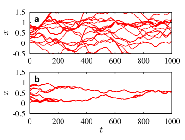
Figure 1: Positions of $25$ particles with viscous dissipation subjected to a spatially and temporally varying random force. The dynamics are described by eqs. (1), (2). In both cases $m=\tau=1$, $\xi=0.05$, $\epsilon=0.001$; a $\gamma\approx 0.04$, b $\gamma\approx 0.1$.

We consider trajectories for a system of independent particles with positions $x_{i}(t)$, and momenta $p_{i}(t)$. The equations of motion for any particle are

$$\dot{x}=p/m\ ,\ \ \ \dot{p}=f(x,t)-\gamma p$$ (1)

where $\dot{x}\!=\!{\rm d}x/{\rm d}t$, and $\gamma$ characterises the strength of the viscous damping. The statistical properties of the force $f(x,t)$ are translationally invariant in both space and time,

$$\langle f(x,t)\rangle\!=\!0\,,\,\,\,\langle f(x,t)f(x^{\prime},t^{\prime})\rangle\!=\!c(x\!-\!x^{\prime},t\!-\!t^{\prime})\,.$$ (2)

$\langle A\rangle$ is the ensemble average of $A$. The correlation function decays rapidly as $|x-x^{\prime}|\to\infty$ and as $|t-t^{\prime}|\to\infty$. A suitable form (adopted in Fig. 1) is $c(\Delta x,\Delta t)\!=\!\epsilon^{2}\exp(-\Delta x^{2}/2\xi^{2})\exp(-\Delta t^{2}/2\tau^{2})$ where $\epsilon$ denotes the magnitude of the force. The dynamics of the model is characterised by two independent dimensionless variables: $\chi\equiv\epsilon\tau^{2}/m\xi$ is a dimensionless measure of the strength of the random force, and the motion is overdamped when $\nu\equiv\gamma\tau\gg 1$.

Phase transition. The phase transition is determined by the fraction of initial conditions for which the separation a pair of infinitesimally close trajectories approaches zero as $t\to\infty$: this is either $0$ or $1$. The separation $\delta x$ of two nearby trajectories has a lognormal distribution. We have

$$\langle{\rm ln}|{\delta x(t)/{\delta x(0)}}|\rangle=\lambda t\,,$$ (3)

we call $\lambda$ the Liapunov exponent. When $\lambda\!<\!0$, almost all nearby trajectories eventually merge, conversely when $\lambda>0$ nearby trajectories almost certainly diverge. The condition for the phase transition is therefore $\lambda=0$, and evaluation of $\lambda$ is also valuable because it gives the rate of coalescence. Linearising the equations of motion (1) gives $\delta\dot{x}=\delta p/m$, and $\delta\dot{p}=-\gamma\delta p+\partial_{x}f(x,t)\,\delta x$. Here $\delta x$ and $\delta p$ are small separations between pairs of trajectories. As $t\to\infty$ the ratio between $\delta p$ and $\delta x$ has a stationary distribution. We therefore write $X=\delta p/\delta x$, and find equations of motion in terms of $X$ and $\delta x$:

$$\delta\dot{x} = X\delta x/m$$ (4)

$$\dot{X} = \partial_{x}f(x(t),t)-\gamma X-X^{2}/m\,.$$ (5)

Since the distribution of $X$ remains stationary, eq. (4) implies that

$$\lambda=\langle X\rangle/m\,.$$ (6)

Consider the dynamics of $X$. When $-X$ is sufficiently large, the noise term $\partial_{x}f\big{(}x(t),t\big{)}$ may be neglected and (5) implies that $X$ reaches $-\infty$ in finite time. This point is a caustic, where $\delta x$ passes through zero and $X$ jumps from $-\infty$ to $+\infty$. As $t\to\infty$, one obtains a stationary distribution, with $X$ going to $-\infty$ at a rate $-J$.

We now specialise to the case where the displacement of $X$ during the correlation time $\tau$ is small compared to the deterministic terms ($\chi\ll 1$), adopting the approach used in hal65 . In this limit the probability density $P(X,t)$ for $X$ satisfies a Fokker-Planck equation Gar90

$$\partial_{t}P=\partial_{X}[(X^{2}/m+\gamma X)P]+{\cal D}\,\partial^{2}_{X}P\,.$$ (7)

with diffusion constant

$${\cal D}=-\frac{1}{2}\frac{\partial^{2}}{\partial x^{2}}\int_{-\infty}^{\infty}{\rm d}t\ c(x,t)\bigg{|}_{x=0}\ .$$ (8)

We require a steady-state solution of eq. (8), $P(X)$, with a constant flux $J$, satisfying $J=v(X)P-{\cal D}{{\rm d}P/{{\rm d}X}}$ with $v(X)=-{X^{2}/m}-\gamma X$. It is convenient to express the solution in terms of dimensionless variables:

$$P(X)=\alpha\,\zeta(Z,\Omega)\ ,\ \ Z={X\over{(m{\cal D})^{1/3}}}\ ,\ \ \Omega={\gamma m^{2/3}\over{{\cal D}^{1/3}}}$$ (9)

where the constant $\alpha$ and function $\zeta$ are to be determined. The exact stationary solution of (7) is

$$\zeta(Z,\Omega)=\exp\bigl{[}-\phi(Z,\Omega)\bigr{]}\int_{-\infty}^{Z}{\rm d}Y\ \exp\bigl{[}\phi(Y,\Omega)\bigr{]}\,.$$ (10)

Here $\phi(Z,\Omega)$ is proportional to the integral of $v(X)$

$$\phi(Z,\Omega)=-\frac{1}{\cal D}\int_{0}^{X}{\rm d}X^{\prime}\ v(X^{\prime})={Z^{3}\over 3}+{\Omega Z^{2}\over 2}\ .$$ (11)

The flux $J$ is determined by normalisation.

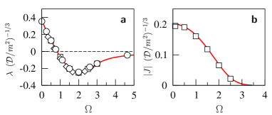
Figure 2: a Liapunov exponent: theory (line) and numerical experiments for $\chi=0.1$ ($\diamond$), $0.02$ ($\Box$), and $0.001$ ($\circ$). b Rate $|J|$ of crossing of caustics, theory (line), and numerical experiments for $\chi=0.02$ ($\Box$).

Using (6) we obtain the Liapunov exponent

$$\lambda=({\cal D}/m^{2})^{1/3}\Psi_{1}(\Omega)/\Psi_{0}(\Omega)$$ (12)

where $\Psi_{n}(\Omega)=\int_{-\infty}^{\infty}{\rm d}Z\ Z^{n}\,\zeta(Z,\Omega)$. The Liapunov exponent is shown in Fig. 2a. Consider the form of (10). When $\Omega$ is large, the integral is approximately constant over the interval between the maximum of $\phi(Z,\Omega)$ at $Z=-\Omega$, and the point $Z={1\over 2}\Omega$ where $\phi$ is equal to its local maximum. In the interval $[-\Omega,{1\over 2}\Omega]$, the function $\zeta(Z,\phi)\sim\beta\exp[-\phi(Z,\Omega]$ for some constant $\beta$. Writing $\zeta(Z,\Omega)=\beta\exp(-\Omega Z^{2}/2)[1-Z^{3}/3+O(Z^{4})]$, we obtain

$$\lambda=-\frac{1}{3}\biggl{(}{{\cal D}\over m^{2}}\biggr{)}^{1/3}\langle Z^{4}\rangle_{0}=-{{\cal D}^{1/3}\over{m^{2/3}\Omega^{2}}}=-{{\cal D}\over{\gamma^{2}m^{2}}}$$ (13)

where $\langle A\rangle_{0}$ defines the average of $A$ with the Gaussian weight, $\zeta_{0}(Z)=\beta\exp(-\Omega Z^{2}/2)$.

Since $\lambda$ is negative for $\Omega\!\gg\!1$, paths coalesce in this regime. When $\Omega\!=\!0$, on the other hand, $\lambda=({\cal D}/m^{2})^{1/3}\sqrt{3}\,\,12^{5/6}\,\Gamma(5/6)/(24\sqrt{\pi})>0$, which establishes the existence of a non-coalescing phase for small $\Omega$ (at $\Omega\!=\!0$ the system is conservative; recent studies scho02 of monodromy matrices for such systems obtain an expression for $\lambda$ equivalent to ours at $\Omega=0$). The transition between the two phases occurs at $\Omega_{\rm c}\approx 0.827$. The two examples shown in Fig. 1 are at $\Omega=0.5$ and $\Omega=1.25$ respectively. The damping which causes the maximum rate of coalescence is determined by the minimum of $\Psi_{1}(\Omega)/\Psi_{0}(\Omega)$: this is at $\Omega\approx 2.035$.

Rate of crossing of caustics. The magnitude of the flux determines the rate at which caustics appear on a given trajectory: $|J|\!=\!({\cal D}/m^{2})^{1/3}/\Psi_{0}(\Omega)$, shown in Fig. 2b. $|J|$ is largest at $\Omega\!=\!0$, $|J|\!=\!({\cal D}/m^{2})^{1/3}\,\Gamma(5/6)\,12^{5/6}/(8\pi^{3/2})$, of the same order at $\Omega_{\rm c}$, and quickly drops to zero at large $\Omega$. In Fig. 1a caustics are still discernible.

Statistics of the particle density. In the overdamped limit ($\nu\gg 1$), the momentum is approximately $p(t)=f(x(t),t)/\gamma$, so that eq. (1) approximated by

$${{\rm d}x(t)\over{{\rm d}t}}={1\over{m\gamma}}f(x(t),t)\ .$$ (14)

In this regime, a more concrete and complete understanding of the path-coalescence effect is obtained by considering the statistics of the density of particles $\varrho(x,t)\!=\!\sum_{i}\delta\bigl{(}x_{i}(t)-x\bigr{)}$. Translational invariance implies that an initially uniform density remains uniform, $\langle\varrho(x,t)\rangle\!=\!\varrho_{0}$. Path coalescence is revealed by the density-density correlation function ${\cal K}(x,x^{\prime};t)\!=\!\big{\langle}\varrho(x,t)\,\varrho(x^{\prime},t)\big{\rangle}\!-\!\varrho_{0}\delta(x-x^{\prime})$. Because of translational invariance, the correlation function ${\cal K}$ is a function of $\Delta x\!=\!x\!-\!x^{\prime}$ only: we write ${\cal K}(x,x^{\prime};t)\!=\!K(\Delta x,t)$. A tendency for particles to cluster is demonstrated by ${K}(\Delta x,t)$ becoming large for $\Delta x$ small, in the limit $t\to\infty$.

When $\chi\ll 1$, we find that the correlation function satisfies a Fokker-Planck equationGar90

$${\partial K(\Delta x,t)\over{\partial t}}={\partial^{2}\over{\partial\Delta x^{2}}}\bigl{[}D(\Delta x)\,K(\Delta x,t)\bigr{]}\ .$$ (15)

The diffusion constant

$$D(\Delta x)={1\over{m^{2}\gamma^{2}}}\int_{-\infty}^{\infty}{\rm d}t\ [c(0,t)-c(\Delta x,t)]$$ (16)

approaches zero quadratically at the origin: $D(\Delta x)\sim\kappa\Delta x^{2}$ for $\Delta x\ll\xi$. When $\Delta x\gg\xi$ the diffusion constant approaches a constant value $D_{0}$.

Now consider the properties of solutions of eq. (15). We note that eq. (15) is in the form of a continuity equation, $\partial K/\partial t+\partial j/\partial\Delta x=0$, so that the integral of the correlation function over all $\Delta x$ is a conserved quantity. The flux of the correlation function passing the separation parameter $\Delta x$ at time $t$ is

$$j(\Delta x,t)=-{\partial\over{\partial\Delta x}}\big{[}D(\Delta x)K(\Delta x,t)\big{]}\ .$$ (17)

Consider an initially uniform distribution of density, with value $\varrho_{0}$ (corresponding to $K(\Delta x,0)=\varrho_{0}^{2}$). For $\Delta x\ll\xi$ the diffusion constant is an increasing function of $\Delta x$. Together with (17) this implies an initial flux of correlation towards $\Delta x=0$. At large times, $K(\Delta x,t)$ is thus sharply peaked at the origin. For $\Delta x\gg\xi$, on the other hand, the approximate solution of (15) is

$$K(\Delta x,t)\sim\varrho_{0}^{2}\,{\rm erf}\biggl{(}{|\Delta x|\over{\sqrt{4D_{0}t}}}\biggr{)}\ .$$ (18)

Using the fact that $K(\Delta x,t)$ satisfies a conservation law, we deduce that the average number of particles condensing into each trail at time $t$ is

$$N(t)\sim{4\over{\sqrt{\pi}}}\varrho_{0}\sqrt{D_{0}t}\ .$$ (19)

When $t/\tau$ is large, and $\Delta x\ll\xi$ (but not too close to zero) the flux $j(\Delta,t)$ is found to be approximately uniform. This implies

$$K(\Delta x,t)\sim{\varrho_{0}^{2}\over{\kappa}}\sqrt{D_{0}\over{\pi}}{1\over{\Delta x\sqrt{t}}}\ .$$ (20)

The $1/X$-divergence of (20) is non-integrable, so that this expression must fail near the origin. An exact calculation shows that $K(0,t)=\exp(2\kappa t)$.

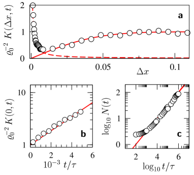
Figure 3: Statistics of $\varrho(x,t)$ in the coalescing phase. a Density correlation $K(\Delta x,t)$ of the process (21): numerical experiments $(\circ)$, limiting theoretical forms (18), full line, and (20), dashed line. Parameter values: $\varepsilon^{2}\approx 1.25\times 10^{-8}$, $\xi\approx 6.4\times 10^{-3}$, and $t=5\times 10^{5}\tau$. b Numerical results verifying that $K(0,t)=\exp(2\kappa t)$ for the same parameter values. c Mean cluster size $N(t)$, of the process (21): numerical experiments ($\circ$), theory (19), line. Parameter values: $\varepsilon^{2}\approx 2\times 10^{-7}$, $\xi\approx 1.6\times 10^{-3}$. Particles are considered to be part of a cluster of $N$ if their positions are within an interval of length $\xi$.

Tracking-minima regime. When $\chi\gg 1$, there is an overdamped phase in which the particles follow minima of the random potential obtained by integrating the force with respect to $x$. A particle executes a rapid jump to a lower minimum whenever the minimum that it has been tracking disappears.

Discrete model. The simplest model exhibiting the path-coalescence effect is a discrete-time random walk which approximates (14):

$$x_{i}(t+\tau)=x_{i}(t)+F_{n}(x_{i}(t))$$ (21)

with $t=n\tau$. By analogy with (2) we take $\langle F_{n}(x)\rangle=0$ and $\langle F_{n}(x)F_{n^{\prime}}(x^{\prime})\rangle=\delta_{nn^{\prime}}C(x-x^{\prime})$. Deutschdeutsch2 gave a detailed analysis of (21). Here we remark that (21) allows us to obtain the simplest possible understanding of why coalescence occurs. Consider the linearisation of (21):

$$\lambda=t^{-1}\,\langle\log|\delta x(t)|/|\delta x(0)|\rangle={\langle\log|1+F^{\prime}_{n}|\rangle/\tau}\,.$$ (22)

When the magnitudes of the derivatives $F^{\prime}_{n}={\rm d}F_{n}/{\rm d}x$ are small compared to unity, Taylor expansion of the logarithm gives $\lambda\sim-{1\over 2}\langle{F_{n}^{\prime}}^{2}\rangle/\tau$, so that $\lambda$ is negative. This approximation is equivalent to (13). This argument indicates that the coalescence is a second-order effect. Also, if the random displacements are larger than their correlation length, the coalescence effect disappears: if $F_{n}$ has a Gaussian distribution, (22) shows that $\lambda$ becomes positive when $\langle{F_{n}^{\prime}}^{2}\rangle$ exceeds $2.421\ldots$. Fig. 3 shows numerical results confirming eqs. (18), (19) and (20), using numerical simulations of the mapping (21).

Applications. In the remainder we discuss a number of possible realisations of the path-coalescence effect.

One example is the motion of liquid droplets on a surface, moving in one direction under a constant force (rain blown off a perspex windshield is an example of this situation). If the surface is randomly contaminated, the wetting angle will be different on opposite sides of each drop, and the trajectory of the droplet will be randomly deflected. We assume the surface contaminants are smeared over an area large compared to that of the droplets (perhaps resulting from cleaning the windshield with a waxy polish), so that nearby droplets are deflected in the same direction. There is no interaction between the drops unless they are close enough to combine due to surface tension: we stress that the coalescence is that of the paths taken by different drops, not of the droplets themselves. We model the motion of a droplet across the surface by a particle of mass $m$. At position ${\bf r}=(x,y)$ on the surface, the drop is subject to a force ${\bf F}({\bf r})+F_{0}\,{\bf j}$, where $F_{0}$ is the magnitude of a steady force acting in the direction of the unit vector ${\bf j}$ defining the $y$-axis and ${\bf F}({\bf r})$ is a homogeneous and isotropic random force with correlation length $\xi$. We assume that the particles are subjected to a viscous resistive force proportional to their velocity across the surface, such that the equations of motion are

$$m{{\rm d}{\bf r}\over{{\rm d}t}}={\bf p}\ ,\ \ \ {{\rm d}{\bf p}\over{{\rm d}t}}=F_{0}\,{\bf j}+{\bf F}({\bf r})-\gamma{\bf p}$$ (23)

(where ${\bf p}$ is the momentum of the drop). When the fluctuating force is weak, the trajectories are locally approximated by straight lines, with $x$ approximately constant and with $y$ increasing at a rate $v_{y}=F_{0}/m\gamma$. The equation of motion in the direction transverse to the constant force is then in the form of equation (1), with $f(x,t)=F_{x}(x,v_{y}t)$. In the case where the motion of the droplets is sufficiently damped, the trajectories coalesce onto fixed trails.

The path-coalescence effect may also be relevant to the motion of energetic electrons in disordered solids. For example, the effect may be relevant to a ‘branching’ observed in the flow of electrons away from a constriction in a two-dimensional electron gas with very low scattering Top01 . The experiment shows regions of markedly increased current density persisting to some distance from the constriction. This was explained by showing similarity to simulations of independent electron motion in the smoothly varying random potential of the doping atoms. This model is essentially (23), with $\gamma=0$. Theoretical discussion of this system Kap02 has emphasised that caustics are important in understanding the empirical results. We remark that these experiments might show an even more pronounced effect if dissipation were introduced. Fig. 1a is similar to the flows discussed in Top01 , showing the branching effect and caustics. Adding dissipation to the electron motion would cause the paths of the electrons to coalesce, as in Fig. 1b. We note that dissipation of the electron motion could be increased by increasing the temperature of the system. As well as giving a criterion for the phase transition, our expression for $J$ also gives a quantitative prediction for the rate of formation of caustics along a given trajectory.

There are also potential applications of the overdamped equations, (14) or (21), in the biological sciences, involving the movement of organisms in response to small random fluctuations in their environment. The model provides a mechanism through which large numbers of organisms can congregate without communicating. One example of this type is the migration of animals across a nearly homogeneous smooth terrain. Thus Fig. 1b could be thought of as a map showing paths of animals on an Eastward migration. The paths of the animals will be deflected by small random fluctuations of topography or vegetation: the animals can be drawn together onto the same paths, even if there is no communication between them, and no gross features in the terrain favouring particular routes. A second example applies to simple organisms such as plankton which can move in response to changes in their environment, such as nutrient concentration. In cases where there are small, spatially correlated random fluctuations of the nutrient concentration, the path-coalescence effect could lead to unexpectedly large concentrations of organisms. Such a mechanism could have been utilised by evolution, enabling simple organisms which cannot communicate directly to congregate for sexual reproduction.

Acknowledgement. Anders Eriksson (Gothenburg University) suggested to us that the path-coalescence effect might be relevant to animal migration patterns. Financial support from Vetenskapsrådet is gratefully acknowledged.

References

- (1) J. Deutsch, J. Phys. A: Math. Gen. 18, 1449 (1985); Phys. Rev. Lett. 52, 1230 (1984).
- (2) B. I. Halperin, Phys. Rev. 139, A104 (1965).
- (3) C. W. Gardiner, Handbook of Stochastic Methods, 2nd ed., Spinger, New York (1990).
- (4) H. Schomerus and M. Titov, Phys. Rev. E 66, 066207 (2002), and references cited therein.
- (5) J. Deutsch, J. Phys. A: Math. Gen. 18, 1457 (1985).
- (6) M. A. Topinka, et al. Nature 410, 183-6, (2001).
- (7) L. Kaplan, Phys. Rev. Lett. 89, 184103 (2002).