Superconductivity from the repulsive electron interaction — from 1D to 3D

Superconductivity from the repulsive electron interaction — from 1D to 3D

An overview is given on how superconductivity with anisotropic pairing can be realised from repulsive electron-electron interaction. (i) We start from the physics in one dimension, where the Tomonaga-Luttinger theory predicts that, while there is no superconducting phase for the repulsive case for a single chain, the phase does exists in ladders with the number of legs equal to or greater than two, as shown both by analytically (renormalisation) and numerically (quantum Monte Carlo). (ii) We then show how this pairing has a natural extension to the two-dimensional case, where anisotropic (usually d) pairing superconductivity arises mediated by spin fluctuations (usually antiferromagnetic), as shown both by analytically (renormalisation) and numerically (quantum Monte Carlo). (iii) We finally discuss how the superconductivity from the electron repulsion can be “optimised” (i.e., how $T_{C}$ can be raised) in 2D and 3D, where we propose that the anisotropic pairing is much favoured in systems having disconnected Fermi surfaces where $T_{C}$ can be almost an order of magnitude higher.

1 Introduction

There is a growing realisation that the high-Tc superconductivity found in the cuprates in the 1980’s has an electronic mechanism — namely, anisotropic pairing from the repulsive electron-electron interaction. Superconductivity from electron repulsion is conceptually interesting in its own right, and has indeed a long history of discussion. In fact, in the field of electron gas, i.e., electron system with the Coulombic electron-electron interaction, Kohn and LuttingerKohnLutt pointed out, as early as in the 1960’s, that the electron gas should become superconducting with anisotropic pairing (having nonzero relative angular momenta) at sufficiently low temperatures in a perturbation theory. This becomes an exact statement for dilute enough electron gas, where p-wave (with the relative angular momentum = 1) should arise, as far as the static interaction is concernedLayzer ; Takadaswave .

While these have to do with the long-range Coulomb interaction where the dominant fluctuation is charge fluctuation, the problem we would like to address here is the opposite limit of short-range repulsion, as appropriate for strongly-correlated systems such as transition metal oxides. There, the dominant fluctuation is the spin fluctuation. The most widely used model is the Hubbard model having the on-site repulsion, $U$. If the one-band Hubbard model, the simplest possible model for repulsively correlated electron systems, superconducts, the interest is not only generic but may be practical as well, which has indeed been a challenge in the physics of high $T_{C}$ superconductivity.

To develop a theory for that, it is instructive to start with one-dimensional (1D) systems. When the system is purely 1D, we have an exact effective theory, which is the Tomonaga-Luttinger theory and is exactly solvable in terms of the bosonisation and renormalisation. So we start with this, where no superconducting phase is shown to exist when the interaction is repulsive. When there are more than one chains, which is called ladders, superconducting phase appears. If one closely looks at the pairing wavefunction, this is a pairing having opposite signs across two bands where the key process is the interband pair hopping.

We then show that this physics has a very natural extension to two-dimensional(2D) systems. There, anisotropic (usually d having the relative angular momentum of 2) pairing superconductivity can arise. If one looks at the pairing wavefunction, this is a pairing having opposite signs across the key interband pair-hopping processes. The key process is dictated by the peak in the spin structure (usually antiferromagnetic).

We finally look at how this kind of anisotropic pairing superconductivity can be “optimised”, namely how we can make $T_{C}$ higher. We first note that “$T_{C}$ is very low in the electron mechanism” in that $T_{C}$ is usually two orders of magnitude lower than the electronic energy. The main reason is the node in the gap function, which has to exist for the anisotropic pairing, intersects the Fermi surface. So we can propose, and show, that systems that have disconnected Fermi surface has much higher $T_{C}$.

2 1D — Tomonaga-Luttinger theory and the physics of ladders

2.1 Tomonaga-Luttinger theory

It was Tomonaga who pioneered the many-body physics in 1D. In his 1950 paperTomonaga the essence of the whole idea is already there, although the theory is now often called Tomonaga-Luttinger. When the system is 1D, the Fermi energy, $E_{F}$, intersects the band at two points, left-moving branch ($L$) and the right-moving one ($R$; Fig.1(a)). The dispersion around these points may be approximated as linear functions of the wavenumber, $k$. When we do this, every electron-hole excitation across $E_{F}$ becomes a creation operator of a sound wave (which is a boson).

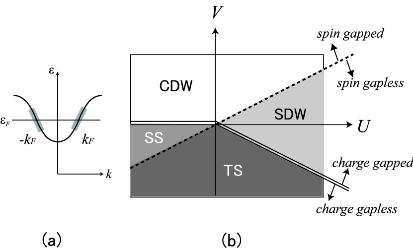
Figure 1: (a) Tomonaga-Luttinger model, in which the low-energy excitations around the Fermi energy (shaded) at $k=\pm k_{F}$ are considered for 1D systems. (b) Weak-coupling result for the phase diagram against the on-site repulsion, $U$, and the off-site repulsion, $V$, for the 1D extended Hubbard model at half filling. SS: spin-singlet superconductivity, TS: triplet superconductivity.

As for the electron-electron interaction, the matrix elements may be classified into four categories: (i) backward scattering, where one electron at $R$ jumps to $L$ while another from $L$ to $R$, (ii) forward scattering, where $R$ jumps to $R$, $L$ jumps to $L$, (iii) umklapp scattering, where ($[R,R]$ jumps to $[L,L]$ or vice versa), (iv) forward scattering within each branch ($[R,R]$ to $[R,R]$ or $[L,L]$ to $[L,L]$). Tomonaga-Luttinger theory  TomLutreview ; weak1 ; weak2 ; weak3 ; weak4 ; weak5 is a weak-coupling theory (i.e., theory for the case when the electron-electron interaction is weak enough), where only question low-energy processes. For that we can integrate out the higher-energy processes in the perturbational renormalisation-group sense. We can then look at the flow of the renormalisation equation, and its end point called the fixed point. To discuss the nature of the fixed-point Hamiltonian, it is convenient to bosonise (i.e., to write everything in terms of boson operators). The final result for the effective Hamiltonian is written in terms of two boson fields, spin phase ($\phi$) and charge phase ($\theta$), whose stiffness (coefficients of $(\partial\phi)^{2},(\partial\theta)^{2}$) is given in terms of only two quantities, $K_{\sigma},K_{\rho}$, which determine everything, including whether the ground state is superconducting. To be more precise, in 1D even a “long-range” order can only have a two-point correlation that decays with a power law ($\propto 1/r^{\alpha}$) where the exponent $\alpha$ is dictated, for each of the order parameters considered, by $K_{\sigma},K_{\rho}$.

For every Hamiltonian originally given, we can calculate the four scattering parameters, and then renormalise them. If we look at the phase diagram (Fig.1(b)) for the extended Hubbard model (where we have an off-site interaction, $V$, on top of the on-site one, $U$), there is no superconducting phase when all the interactions $U$ and $V$ are repulsive ($>0$).

Incidentally, there is no magnetism, either, for a single chain. This is due to the well-known Lieb-Mattis theorem, which dictates that electrons in 1D are entirely non-ferromagnetic. The proof makes use of the fermion statistics of electrons, where a key factor is no two electrons can pass each other in 1D, or, in the words in Mattis’s textbookMattis , “neighbours remain neighbours till death did them part”.

2.2 Pairing in ladders, or $1+1\neq 2$

When there are more than one chain with inter-chain hopping and/or interaction, the physics can be, and is indeed, entirely different. The model, then, becomes multi-band (i.e., $n$-band system for $n$-leg ladder). The Fermi energy can intersect the dispersion at $2n$ points (Fig.2), so the model is what can be called multiband Tomonaga-Luttinger model. The multiband Tomonaga-Luttinger model has been studied in various context, including the excitonic phase in electron-hole systemsnagaosaogawa , transport propertiesspinpolTL and interband excitations in quantum wires as detected by Raman spectroscopy by Sassetti et al.sassetti

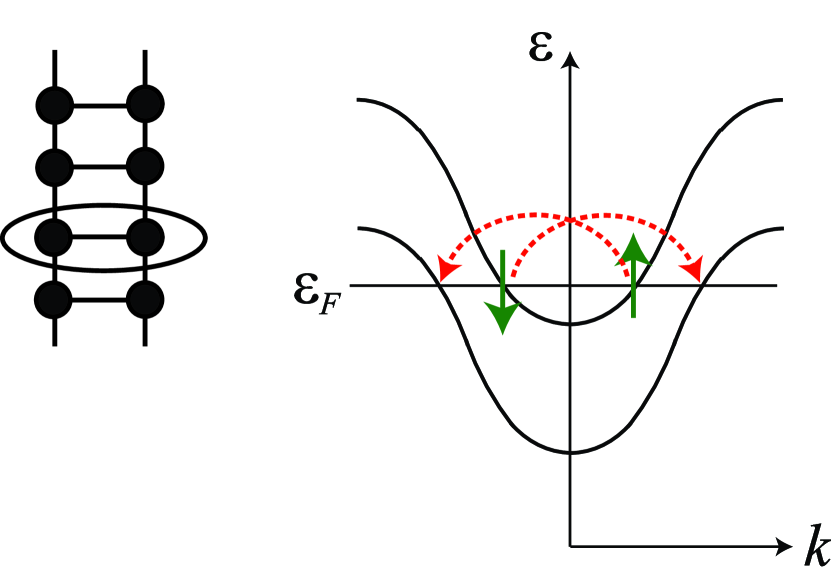
Figure 2: Multi-band 1D model (right panel) for the Hubbard model on a ladder (left). An oval on the ladder represents the inter-chain pairing.

In the context of the high $T_{C}$, the idea of superconductivity in multi-chain (or “ladder”) systems was kicked off theoretically in 1986, when Schulz SchulzAF proposed a possible relation between ladders at half-filling and Haldane’s conjecture for spin chains. He made the following reasoning: If we consider repulsively interacting electrons on a ladder, the undoped system will be a Mott insulator, so that we may consider the system as an $S=1/2$ antiferromagnetic (AF) Heisenberg magnet on a ladder for large Hubbard repulsion $U$. Schulz’s analysis SchulzAF is that an AF $S=n/2$ single chain, which is exactly the Haldane’s system Haldane ; Nishiyama , is similar to an $S=1/2$ AF ladder with $n$-legs. For the spin chains, Haldane Haldane has conjectured that the spin excitation should be gapless for half-odd-integer spins ($n$: odd) or gapful for integer spins ($n$: even). If the situation is similar in ladders, a ladder having an even number of legs will have a spin gap, associated with a ‘spin-liquid’ ground state where the quantum fluctuation is so large that the AF correlation decays exponentially.

Dagotto et al.Dagotto1 and by Rice et al.Rice , then suggested the possibility of superconductivity associated with the spin gap. The presence of a spin gap, i.e., a gap in the spin excitation which is indicative of a quantum spin liquid, in the two-leg ladder (or, more generally, in even legs) is a good news for superconductivity, since an idea proposed by Anderson Anderson in the context of the high-$T_{C}$ superconductivity suggests that a way to obtain superconductivity is to carrier-dope spin-gapped systems. The superconductivity in even-leg ladders is in accord with this. Subsequently superconductivity has been reported for a cuprate with a ladder structureUehara , although it later turned out that this material has a rather strong two-dimensionality that may dominate the superconductivity.

For doped systems, the conjecture for superconductivity Rice is partly based on an exact diagonalisation study for finite $t$-$J$ model on a two-leg ladder. Dagotto This was then followed by analytical Sigrist and numerical Poilblanc3 ; Tsunetsugu ; Hayward ; Sano works on the doped $t$-$J$ ladder, for which the region for the dominant pairing correlation appears at lower side of the exchange coupling $J$ than in the case of a single chain.

On the other hand the Hubbard model on a ladder is of general interest.KAmultiTL Although the Hubbard crosses over to the $t$-$J$ model for $U\rightarrow\infty$, we have only an infinitesimal $J$ there, so the result for $t$-$J$ model does not directly answers this. Since there is no exact solution for the Hubbard ladder, we can proceed in two ways: for small $U$ we can adopt an analytic method, which is the weak-coupling renormalisation-group theory, where the band structure around the Fermi points is linearised in the continuum limit to treat the interaction with a perturbative renormalisation group. The weak-coupling theory with the bosonisation and renormalisation-group techniques has been applied to the two-leg Hubbard ladder.  Finkelstein ; Balents ; Fabrizio ; Fab ; Nagaosa ; Schulz2

The Hamiltonian of the two-leg Hubbard ladder is given in standard notations as

$${\cal H} = -t\sum_{\alpha\langle i\rangle\sigma}(c_{i\sigma}^{\alpha\dagger}c^{\alpha}_{i+1\sigma}+{\rm h.c.})-t_{\perp}\sum_{i\sigma}(c_{i\sigma}^{1\dagger}c^{2}_{i\sigma}+{\rm h.c.})$$ (2)

$$+U\sum_{\alpha i}n^{\alpha}_{i\uparrow}n^{\alpha}_{i\downarrow},$$

where $\alpha(=1,2)$ specifies the chains, or in the momentum space as

$${\cal H} = -2t\sum_{\mu k\sigma}\cos(k)c^{\mu\dagger}_{k\sigma}c^{\mu}_{k\sigma}-2t_{\perp}\sum_{k\sigma}c^{0\dagger}_{k\sigma}c^{0}_{k\sigma}$$ (4)

$$+U\sum({\rm interaction\>\>of\>\>the\>\>form}\>\>c^{\dagger}c^{\dagger}cc),$$

where $\mu$ specifies the bonding ($\mu=0$) and anti-bonding ($\mu=\pi$) bands, so labelled since $k_{y}=0,\pi$, respectively.

The part of the Hamiltonian, $H_{\rm d}$, that can be diagonalised in the bosonisation includes only intra- and inter-band forward-scattering processes arising from the intrachain forward-scattering terms. We can then define bosonic operators as in the single-chain case. If we introduce the phase variables as in the single-chain case, $H_{\rm d}$, written in terms of them, is separated into the spin-part $H_{\rm spin}$ and the charge-part $H_{\rm charge}$. While $H_{\rm spin}$ is already diagonalised, $H_{\rm charge}$ can be made so with a linear transformation, and the diagonalised $H_{\rm charge}$ is written in terms of the correlation exponent $K_{\rho i},i=1,2$. So we end up with the total Hamiltonian that reads

$$H={\rm kineticenergy}+H_{{\rm d}}+\mbox{pair-hopping terms}.$$ (5)

Here, the pair-hopping (or pair-scattering) term represents those part of the interaction Hamiltonian, in which a pair of electrons is scattered via the interaction to another pair of electrons.

At half-filling, the system reduces to a spin-liquid insulator having both charge and spin gaps Balents . When carriers are doped to the two-leg Hubbard ladder, on the other hand, the relevant scattering processes at the fixed point in the renormalisation-group flow are the pair hopping across the bonding and anti-bonding bands (Fig.2), $c_{\uparrow}^{\pi\dagger}c_{\downarrow}^{\pi\dagger}c_{\downarrow}^{0}c_{\uparrow}^{0}+{\rm h.c.}$ in $k$ space, and the backward-scattering process within each band. The importance of the pair-hopping across the two bands for the dominance of pairing correlation in the two-leg Hubbard ladder is reminiscent of the Suhl-Kondo mechanism, which was proposed back in the 1950’s for superconductivity in a quite different context of the s-d model for the transition metals. Suhl ; Kondo

The renormalisation results in a formation of gaps in both of the two spin modes and a gap in one of the charge modes. This leaves one charge mode massless, where the mode is characterised by a critical exponent $K_{\rho}$. Then the correlation of the intraband singlet pairing,

$$\sum_{\sigma}\sigma(c_{k\sigma}^{0}c_{-k,-\sigma}^{0}-c^{\pi}_{k\sigma}c^{\pi}_{-k,-\sigma}),$$ (6)

decays like $1/r^{1/(2K_{\rho})}$, where $K_{\rho}$ should be close to unity in the weak-coupling regime. So this should be the dominant phase, which is, expressed in real space as $c^{1}_{i\sigma}c^{2}_{i,-\sigma}-c^{1}_{i,-\sigma}c^{2}_{i\sigma}$, an interchain singlet pairing.

2.3 How to detect pairing in quantum Monte Carlo studies?

The perturbational renormalisation group is in principle guaranteed to be valid only for sufficiently small interaction strengths ($U\ll t$), so that its validity for finite $U(\sim t$) has to be checked. To be more precise, the renormalisation approach can tell whether the interaction flows into weak coupling (with the relevant mode gapless) or into strong-coupling regime (gapful) for small enough interactions, but the framework itself (i.e., the perturbational expansion) might fail for stronger interactions.

This is where numerical studies come in. Numerical calculations for finite $U$ have been performed with the exact diagonalisation, DMRG or quantum Monte Carlo (QMC) methods, Hirsch ; MC1 ; MC2 ; MC3 ; MC4 ; MC5 but in an earlier stage the results are scattered, where some of the results seemed inconsistent with the weak-coupling prediction: a DMRG study by Noack et al. for the doped Hubbard ladder shows the enhancement of the pairing correlation over the $U=0$ result strongly depends on the inter-chain hopping, $t_{\perp}$Noack1 ; Noack2 . Quantum Monte Carlo (QMC) results also exhibit an absenceAsai or presenceYamaji of the enhancement depending on the hopping parameters and/or band filling.

Recently, however, a QMC study by Kuroki et al Kuroki has resolved the puzzle, and has clearly detected an enhanced pairing correlation. A key factor found there in detecting superconductivity in any numerical calculation, which also resolves the origin of the former discrepancies is: we have to question a very tiny energy scale ($\ll$ starting electronic energy scale, $t,U$) in detecting the pairing. This immediately implies that the discreteness of energy levels in finite systems examined in QMC studies enormously affects the pairing correlation — If the level separation is greater than the energy scale we want to look at, any feature in the correlation function will be easily washed out. This can be circumvented if we tune the parameters so as to make the separation between the levels just below and above $E_{F}$ tiny (i.e., to make the LUMO-HOMO nearly degenerate in the quantum chemical language), which should be a reasonable way to approach the bulk limit where the levels are dense. The importance of small offsets between the highest occupied and lowest unoccupied levels has also been stressed by Yamaji et al. for small systems. Yamaji

So we have applied the (projector) Monte Carlo methodpmc to look into the ground state correlation function $P(r)\equiv\langle O_{i+r}^{\dagger}O_{i}\rangle$ of this pairing for finite values of $U(\sim t)$. We show in Fig.3 the result for $P(r)$ for $t_{\perp}=0.98$, $U=1$ and the band filling $n=0.867=52$ electrons/ (30 rungs $\times$ 2 sites). The $U=0$ result (dashed line) for these two values of $t_{\perp}$ are identical because the Fermi sea remains unchanged. If we turn on $U$, we can see that a large enhancement over the $U=0$ result emerges at large distances.

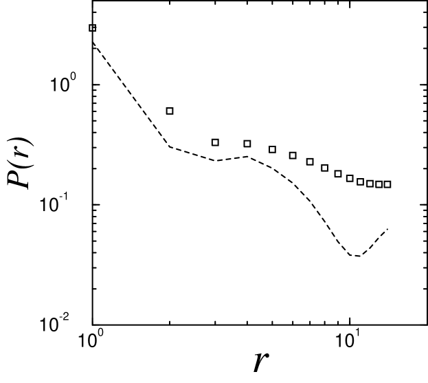
Figure 3: The pairing correlation function plotted against the real space distance $r$ in a 30-rung Hubbard ladder having 56 electrons for $U=1$ with $t_{\perp}=1.975$ (square).Kuroki The dashed line is the non-interacting result.

We have deliberately chosen the value of $t_{\perp}=0.98$ to make the one-electron energy levels of the bonding and anti-bonding bands lie close to each other around the Fermi level within $0.004t$. This is much smaller than the energy scale we question (which is the spin gap in the present 1D case). In fact, a 5% change in $t_{\perp}=0.98\rightarrow 1.03$, for which the LUMO-HOMO separation blows up to $\sim 0.1t$, washes out the enhancement in the correlation function. In the latter case the renormalisation of higher energy modes has to stop at this energy scale, so that the interband pair hopping process will not be renormalised into a strong coupling, while in the weak-coupling theory the renormalisation all the way down to the Fermi level is assumed.

While it is difficult to determine the decay exponent of the pairing correlation $P(r)$, we can fit the data by assuming a trial function expected from the weak-coupling theory, $P(r)\propto c/\sqrt{r}+(1-c)/r^{2}+[\cos(2k_{F}^{0}r)+\cos(2k_{F}^{\pi}r)]/r^{2}$ where the overall decay at large distances is assumed to be $\propto 1/\sqrt{r}$ as dictated in the weak-coupling theory. This form reproduces the result surprisingly accurately.

3 Three-leg ladder and 1D-2D crossover

Now, the physics of ladders can provide quite an instructive line of approach for understanding the physics in two-dimensional systems via the crossover from 1D to 2D (two-dimensions). So let us first look at the three-leg ladder.

3.1 Three-leg ladder

If we return to ladders, one can naively expect that ladders with odd-number (e.g., 3) of legs will have no spin gap, which would then signify an absence of dominating pairing correlation (‘even-odd conjecture for superconductivity’). As far as the spin gap in undoped ladders is concerned, experiments on a class of cuprates, Sr_n-1Cu_nO_2n-1 having $n$-leg ladders, have supported the conjecture. Azuma ; Ishida1 ; Kojima ; Hiroi2 ; Mayaffre So it was believed that odd-numbered legs only have the usual $2k_{F}$ spin-density wave (SDW) rather than superconductivity.

Kimura et alTakashi1 ; Takashi2 ,however, showed that that is too simplistic a view, and that, while the even-odd conjecture for the spin gap is certainly correct, an odd-number of legs does indeed superconduct by exploiting the spin-gapped mode. In that work the pairing correlation in the three-leg Hubbard ladder has been examinedtJcom .

We start with the weak-coupling theory for correlation functions for the three-leg Hubbard ladder (Fig.4). Arrigoni has looked into a three-leg ladder with weak Hubbard-type interactions with the perturbational renormalisation-group technique to conclude that gapless and gapful spin excitations coexist in three legs. Arrigoni

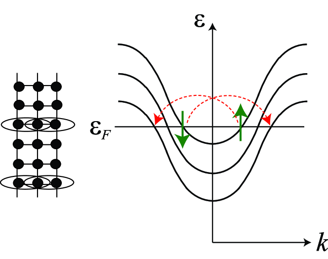
Figure 4: Three-leg ladder (inset) and its dispersion. The dashed arrows represent the pair-hopping process, and ovals represent the inter-chain pairing.

He has actually enumerated the numbers of gapless charge and spin modes on the phase diagram spanned by the doping level and the interchain hopping, $t_{\perp}$. He found that, at half-filling, one gapless spin mode exists. For general band filling, one gapless spin mode remains in the region where the Fermi level intersects all the three bands in the noninteracting case. From this, Arrigoni argues that the $2k_{F}$ SDW correlation should decay as a power law as expected from experiments. Arrigoni’s result indicates that two gapful spin modes exist in addition. The charge modes, on the other hand, consists of two gapless modes and one gapful mode.

The question we address then is what happens when gapless and gapful spin modes coexist. This is an intriguing problem, since it may well be possible that the presence of gap(s) in some out of multiple spin modes may be sufficient for the dominance of a pairing correlation. Schulz Schulz3 has independently shown similar results for a subdominant $2k_{F}$ SDW and the interchain pairing correlations.

Physically, the picture that emerges as we shall describe below, is that the two spin gaps, which are relevant to the pairing, arise as an effect of the pair-hopping process that is the many-body matrix element transferring two electrons simultaneously across the outermost bands (i.e., the top and bottom bands for a three-leg ladder) (Fig.4). In this sense the mechanism is reminiscent of the situation in the two-leg case or the Suhl-Kondo mechanism. Suhl ; Kondo

The correlation functions can be calculated with the bosonisation method TomLutreview for the three-leg Hubbard model.

We can define three bosonic operators, where we diagonalise $H_{\rm charge}$ in terms of the three correlation exponents $K_{\rho i},i=1,2,3$. As Arrigoni pointed out Arrigoni the pair-hopping processes across the top and bottom bands become relevant as the renormalisation is performed. In order to actually calculate the correlation functions, we have to express the relevant scattering processes in terms of the phase variables. The fixed-point Hamiltonian density, $H^{*}$, takes the form, in terms of the phase variables,

$$H^{*}\propto - g_{\rm back}(1){\rm cos}[2\phi^{1+}(x)]-g_{\rm back}(3){\rm cos}[2\phi^{3+}(x)]$$ (7)

$$+ 2g_{\rm pairhopping}(1,3){\rm cos}[\sqrt{2}\chi^{1-}(x)]{\rm sin}\phi^{1+}(x){\rm sin}\phi^{3+}(x),$$ (8)

where $g_{\rm back}(1),g_{\rm back}(3)$ are negative large quantities, and $g_{\rm ph}(1,3)$ is a positive large quantity. This indicates the following. Two spin phases, $\phi^{1+}$, $\phi^{3+}$, become long-range ordered and fixed, respectively, while $\phi^{2+}$ is not fixed to give a gapless spin mode. Similarly, the difference in the charge phases, $\theta^{i}$, for the outermost bands,

$$\chi^{1-}\equiv\frac{1}{\sqrt{2}}(\theta^{1-}-\theta^{3-}),$$ (9)

is ordered and fixed, and the charge gap opens for this particular mode.

Now we can calculate the correlation functions, since the gapless fields have already been diagonalised, while the remaining gapful fields have the respective expectation values.

Among various order parameters, the dominant one (with the longest tail in the correlation) is the singlet pairing across the central and edge chains (Fig.4), which is, in the band picture,

$$O_{d}\sim\sum_{\sigma}\sigma(\psi^{1+}_{\sigma}\psi^{1-}_{-\sigma}-\psi^{3+}_{\sigma}\psi^{3-}_{-\sigma}).$$ (10)

We call this “d” for the following reason. Since we have taken a continuum limit along the chain, it is not straightforward to name the symmetry of a pairing. However, we could call the above pair as d-wave-like in that the pairing, in addition to being off-site on the rung, is a linear combination of a bonding band and an anti-bonding band with opposite signs. Since the relevant pair-hopping is across these bands, we can say that there is a node in the pair wavefunction along the line that bisects the relevant pair-hopping.

Calculation of the correlation function of $O_{d}$ gives

$$\langle O_{d}(x)^{\dagger}O_{d}(0)\rangle\sim x^{-\frac{1}{3}(\frac{1}{K_{\rho 2}^{*}}+\frac{1}{2K_{\rho 3}^{*}})},$$ (11)

which is the dominant ordering. In the weak-interaction limit ($U\rightarrow+0$), where all the $K^{*}$’s tend to unity, the “d”-pairing correlation decays as slowly as $x^{-1/2}$, while the other correlations decay like $x^{-2}$. We can see that the interchain pairing exploits the charge gap and the spin gaps to reduce the exponent of the correlation function, in contrast to the intrachain pairing. Namely, we would have ($-1$) in the exponent if the spin were gapless. This alone would only result in a $1/r$ decay, but the charge mode $\chi_{1-}$ is further locked, which further reduces the exponent (down to $1/\sqrt{r}$ in the limit $U\rightarrow 0$).

Now, how the pairing correlation in the three-leg Hubbard ladder looks like when $U$ is finite? Our QMC result for the three-leg Hubbard ladder exhibits an enhancement of the pairing correlation even for finite coupling constants, $U/t=1\sim 2$. Takashi2 As in the two-leg case with a finite $U$, we have taken care that levels below and above the Fermi level are close.

3.2 1D-2D crossover

We have seen that the weak-coupling theory (perturbational renormalisation + bosonisation) predicts that the interband pair hopping between the innermost and outermost Fermi points $(k_{x},k_{y})\approx(\pm k_{F}^{0},0),(\pm k_{F}^{\pi},\pi)$ becomes relevant (i.e., increases with the renormalisation). This concomitantly makes the two-point correlation of the interchain singlet decay slowly with distance. In $k$-space the dominant component of this pair reads

$$\sum_{\sigma}\sigma\ (c_{k_{F}^{0},\sigma}^{0}c_{-k_{F}^{0},-\sigma}^{0}-c_{k_{F}^{\pi},\sigma}^{\pi}c_{-k_{F}^{\pi},-\sigma}^{\pi}).$$ (12)

Now, when $E_{F}$ intersects the outermost-band top and the innermost-band bottom with $k_{F}^{0}\simeq\pi,k_{F}^{\pi}\simeq 0$ (Fig.5 left), intrachain nearest-neighbor singlet pair also has a dominant Fourier-component equal to eqn.(12) with a phase shift $\pi$ relative to the interchain pairing. Thus, a linear combination which amounts to the d${}_{x^{2}-y^{2}}$ pairing should become dominant. We shall see this is exactly what happens in the 2D squre lattice around the half filling, Fig.5 right.

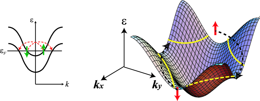
Figure 5: Band dispersion of the square lattice, on which the Fermi surface for $E_{F}$ close to half filling and a typical pair-hopping process (dashed arrows) are shown. Similar plot for a ladder is attached for comparison.

4 Superconductivity from the repulsive interaction in 2D

As we have seen, the two-leg and three-leg Hubbard ladders do superconduct, so what will happen if we consider $n$-leg ladders for $n=3,4,...,\infty$ to reach the 2D square lattice. This view enables us to have a fresh look at the 2D Hubbard model.

So we move on to the repulsive Hubbard model on the square lattice. The seminal notion that the high-$T_{C}$ conductivity in cuprates should be related the strong electron correlation was first put forward by Anderson.Andersonreview There the superconductivity is expected to arise from the pairing interaction mediated by spin fluctuations (usually antiferromagnetic). A phenomenology along this line such as the self-consistent renormalisation Moriya1 ; Moriya2 ; Moriya3 ; Pines1 has succeeded in reproducing anisotropic $d$-wave superconductivity. Microscopically, the repulsive Hubbard model, a simplest possible model for correlated electrons, should capture the physics in cuprates.dpKA Some analytical calculations have suggested the occurrence of d${}_{x^{2}-y^{2}}$-wave superconductivity in the 2D Hubbard model. Bickers ; Dzyalo ; Schulz ; ScalapinoPhysRep ; Alvarez In particular, fluctuation exchange approximation (FLEX), developed by Bickers et al.FLEX , has also been applied to the Hubbard model on the square lattice Dahm ; Deisz to show the occurrence of the superconductivity.

Numerical calculations have also been performed extensively. Finite binding energyDMST ; FOP and pairing interaction vertexWhite ; Husslein ; Zhang were found in those calculations. Variational Monte Carlo calculations show that a superconducting order lowers the variational energy.Giamarchi ; YamajiVMC Nevertheless, there had been a reservation against the occurrence of superconductivity in the Hubbard model because the pairing correlation functions do not show any symptom of long-range behavior in some of the works.Zhang ; Furukawa ; Moreo

Again, Kuroki et alKuroki showed for the first time that QMC does indeed exhibit symptoms of superconductivity if we take proper care of a small energy scale involved, i.e., the d-wave pairing correlation becomes long-tailed when the Fermi level lies between a narrowly separated levels residing on the k-points across which the dominant pair hopping occurs. An enhancement of the pairing correlation has in fact been found by exact diagonalisationYamaji and by density matrix renormalisation groupNoack2 when $E_{F}$ lies close to the $k$-points $(0,\pi)$ and $(\pi,0)$. Although the d${}_{x^{2}-y^{2}}$-like nature of the pairing was suggested,Noack2 d${}_{x^{2}-y^{2}}$ pairing correlation itself has not been calculated. So, in our quest for 2D, we first calculate the correlation function with QMC. Here we employ the ground-state, canonical-ensemble QMC,stab where we take the free Fermi sea as the trial state.

4.1 Anisotropic pairing in 2D

First, let us look at why the attractive interaction is by no means a necessary condition for superconductivity, which can quite generally arise from repulsive electron-electron interactions, which seems to be still not realised well enough. If we look at the BCS gap equation, we can immediately see that superconductivity can readily arise from repulsive interactions. The gap equation reads

$$1 = -V_{\phi}\sum_{\mbox{\boldmath$k$}^{\prime}}\frac{1}{2\varepsilon(\mbox{\boldmath$k$}^{\prime})}{\rm tanh}\left[\frac{1}{2}\beta\varepsilon(\mbox{\boldmath$k$}^{\prime})\right],$$ (14)

$$V_{\phi}=\frac{\langle V(\mbox{\boldmath$k,k$}^{\prime})\Delta(\mbox{\boldmath$k$})\Delta(\mbox{\boldmath$k$}^{\prime})\rangle_{\rm FS}}{\langle\Delta^{2}(\mbox{\boldmath$k$})\rangle_{\rm FS}},$$

where $\varepsilon(\mbox{\boldmath$k$})$ is the band energy measured from the chemical potential, $\beta=1/(k_{B}T_{C})$, $V(\mbox{\boldmath$k,k$}^{\prime})$ the pair-hopping matrix element, $\Delta(\mbox{\boldmath$k$})$ the BCS gap function, and $\langle...\rangle_{\rm FS}$ is the average over the Fermi surface. So, if $\Delta(\mbox{\boldmath$k$})$ has nodes across $\mbox{\boldmath$k$}\leftrightarrow\mbox{\boldmath$k$}^{\prime}$ (i.e., changes sign before and after the pair hopping), the originally repulsive $V>0$ acts effectively as an attraction,

$$\langle V(\mbox{\boldmath$k,k$}^{\prime})\Delta(\mbox{\boldmath$k$})\Delta(\mbox{\boldmath$k$}^{\prime})\rangle_{\rm FS}<0.$$

This most typically happens for the $d_{x^{2}-y^{2}}$ pairing with $\Delta(\mbox{\boldmath$k$})\propto{\rm cos}(k_{x})-{\rm cos}(k_{y})$ when the dominant pair hopping occurs across $\mbox{\boldmath$k$}\sim(0,\pi)\leftrightarrow\mbox{\boldmath$k$}^{\prime}\sim(\pi,0)$.

When the spin fluctuation is antiferromagnetic, most typically in bipartite lattices such as a square lattice, the importance of the interactions around $(0,\pi)$ and $(\pi,0)$ in the 2D Hubbard model has been suggested by various authors. Dzyalo ; Schulz ; ScalapinoPhysRep ; Alvarez ; Husslein ; YamajiVMC ; LeeRead ; Newns ; Mark ; Gonzalez

Group theoretically, the square lattice has a tetragonal symmetry, so that everything, including the gap function, should be an irreducible representation of the tetragonal group. The $d_{x^{2}-y^{2}}$ pairing indeed belongs to B_1g representation of this group.

4.2 Quantum Monte Carlo study for the 2D Hubbard model

In the context of our QMC study for the 2D Hubbard model, we have to take finite systems that have the $k$-points around $(0,\pi)$ and $(\pi,0)$ close in energy. Nameley, our expectation from the study on ladders is that the pair hopping processes across around $(0,\pi)$ and $(\pi,0)$ may result in d${}_{x^{2}-y^{2}}$ pairing, $\sum_{\mbox{\boldmath$k$}}[{\rm cos}(k_{x})-{\rm cos}(k_{y})]c_{\mbox{\boldmath$k$}\uparrow}c_{-\mbox{\boldmath$k$}\downarrow}$ in 2D, but an enhanced pairing correlation should be detected only when the level offset between the discrete levels around those points is small.

We take 78 electrons in $10\times 10$ sites ($n=0.78$) with $t_{y}=0.999$ with periodic boundary condition in both directions. We have taken $t_{y}=0.999$, because the number of electrons considered here would have an open shell (with a degeneracy in the free-electron Fermi sea) for $t_{y}=1$, which will destabilise QMC convergence. Taking $t_{y}=0.999$ lifts the degeneracy to give a tiny ($<0.01$) but finite $\Delta\varepsilon^{0}$. In Fig.6 we plot the d${}_{x^{2}-y^{2}}$ pairing correlation, defined as

$$P(r) = \sum_{|\Delta x|+|\Delta y|=r}\langle O^{\dagger}(x+\Delta x,y+\Delta y)O(x,y)\rangle,$$ (15)

$$O(x,y) = \sum_{\delta=\pm 1,\sigma}\sigma(c_{x,y,\sigma}c_{x+\delta,y,-\sigma}-c_{x,y,\sigma}c_{x,y+\delta,-\sigma}),$$ (16)

where the correlation for $U=1$ is clearly seen to be enhanced over that for $U=0$ especially at large distances.

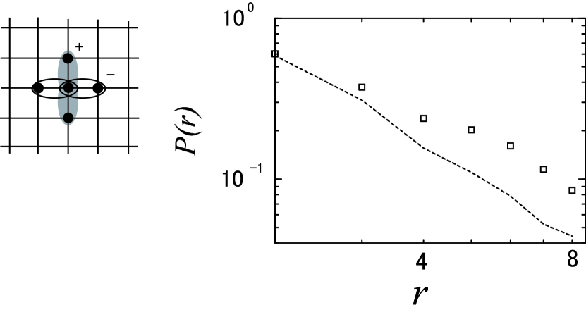
Figure 6: QMC result for the d${}_{x^{2}-y^{2}}$ pairing correlation for a $10\times 10$ square lattice with 78 electrons for $U=1$ and $t_{y}=0.999$ (square).Kuroki The dashed line represents the noninteracting case. Inset depicts the square lattice with the ovals representing a d-wave pair.

We can readily show that when the level spacing becomes too large (e.g., $\Delta\varepsilon^{0}\sim 0.1$), the enhancement is washed out. In the present choice the energy levels around $(0,\pi),(\pi,0)$ are close ($<0.01t)$, while the other levels lie more than $\sim 0.1t$ away from $E_{F}^{0}$. One might thus raise a criticism that the scattering processes involving the states away from $E_{F}^{0}$ are unduly neglected. We can however show (not displayed here) that when other levels exist around $E_{F}$ an enhanced d${}_{x^{2}-y^{2}}$ correlation is obtained as well.

How about the band-filling ($n$) dependence? We have calculated the long-range part of the correlation, $S\equiv\sum_{r\geq 3}P(r)$, for various values of $n$ keeping $\Delta\varepsilon^{0}<0.01t$ throughout. The result, displayed in Fig.7, shows that the enhancement in $S$ for $U=1$ has a maximum around a finite doping. Thus the message here is that the d${}_{x^{2}-y^{2}}$ pairing is favoured near, but not exactly at, half-filling. The fact that the better nesting does not necesarrily imply the more enhanced pairing correlation has also been shown in another numerical work in the contex of an organic superconductivity.KAorganic

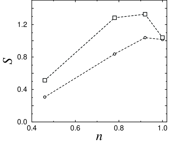
Figure 7: The integrated pairing correlation plotted against the band filling $n$ for a $10\times 10$ lattice with $U=0$ $(\circ)$ or $U=1$ (square).Kuroki

5 Which is more favourable for superconductivity, 2D or 3D?

The theoretical results described so far indicate that the superconductivity near the AF instability in 2D has a ‘low $T_{C}$’ $\sim O(0.01t)$ ($t$: transfer integral), i.e., two orders of magnitude smaller than the original electronic energy, but still ‘high $T_{C}$’ $\sim O(100$ K) for $t\sim O(1$ eV). So, identifying the conditions for higher $T_{C}$ in the repulsive Hubbard model is one of the most fascinating goals of theoretical studies. For instance, while the high-$T_{C}$ cuprates are layer-type materials with Cu₂ planes in which the supercurrent flows, the question is whether the two-dimensionality is promoting or degrading the superconductivity.

Hence Arita et al2d3d have questioned: (i) Is 2D system more favourable for spin-fluctuation mediated superconductivity than in three dimensions(3D)? (ii) Can other pairing, such as a triplet $p$-pairing in the presence of ferromagnetic spin fluctuations, become competitive? We take the single-band, repulsive Hubbard model as a simplest possible model, and look into the pairing with the FLEX method in ordinary (i.e., square, trianglar, fcc, bcc, etc) lattices in 2D and 3D. The FLEX method has an advantage that systems having large spin fluctuations can be handled.

As for 3D systems, Scalapino et alScalapino showed for the Hubbard model that paramagnon exchange near a spin-density wave instability gives rise to a strong singlet $d$-wave pairing interaction, but $T_{C}$ was not discussed there. Nakamura et alNakamura extended Moriya’s spin fluctuation theory of superconductivityMoriya2 to 3D systems, and concluded that $T_{C}$ is similar between the 2D and 3D cases provided that common parameter values (scaled by the band width) are taken. However, the parameters there are phenomelogical ones, so we wish to see whether the result remains valid for microscopic models.

As for the triplet pairing, the possibility of triplet pairing mediated by ferromagnetic fluctuations has been investigated for superfluid ${}^{3}{\rm He}$Leggett , a heavy fermion system ${\rm UPt_{3}}$heavyFermion , and most recently, an oxide ${\rm Sr_{2}RuO_{4}}$Sr . It was shown that ferromagnetic fluctuations favour triplet pairing first by Layzer and FayLayzer before the experimental observation of p-wave pairing in ${}^{3}{\rm He}$. For the electron gas model, Fay and LayzerLayzer and later ChubukovChubukov has extended the Kohn-Luttinger theoremKohnLutt to $p$-pairing for 2D and 3D electron gas in the dilute limit. TakadaTakada discussed the possibility of $p$-wave superconductivity in the dilute electron gas with the Kukkonen-Overhauser modelKO . As for lattice systems, 2D Hubbard model with large enough next-nearest-neighbor hopping $(t^{\prime})$ has been shown to exhibit $p$-pairing for small band fillings.ChubukovLu HlubinaHlubina99 reached a similar conclusion by evaluating the superconducting vertex in a perturbative way.Takahashi However, the energy scale of the $p$-pairing in the Hubbard model, i.e., $T_{C}$, has not been evaluated so far.

Here we show that (i) $d$-wave instability mediated by AF spin fluctuation in 2D square lattice is much stronger than those in 3D, while (ii) $p$-wave instability mediated by ferromagnetic spin fluctuations in 2D are much weaker than the $d$-instability. These results, which cannot be predicted a priori, suggest that for the Hubbard model the ‘best’ situation for the pairing instability is the 2D case with dominant AF fluctuations.

We consider the single-band Hubbard model with the transfer energy $t_{ij}=t(=1$ hereafter) for nearest neighbors along with $t_{ij}=t^{\prime}$ for second-nearest neighbors, which is included to incorporate the band structure dependence. The FLEX starts from a set of skeleton diagrams for the Luttinger-Ward functional to generate a ($k$-dependent) self energy based on the idea of Baym and KadanoffBaym . Hence the FLEX approximation is a self-consistent perturbation approximation with respect to on-site interaction $U$.

To obtain $T_{C}$, we solve the eigenvalue (Éliashberg) equation,

$$\lambda\Sigma^{(2)}(k) = \frac{T}{N}\sum_{k^{\prime}}\Sigma^{(2)}(k^{\prime})|G(k^{\prime})|^{2}V^{(2)}(k-k^{\prime}),$$ (17)

where $\Sigma^{(2)}(k)$ is the anomalous self energy, $k\equiv(\mbox{\boldmath$k$},i\omega_{n})$ with $\omega_{n}=(2n-1)\pi T$ being Matsubara frequencies, and the pairing interaction, $V^{(2)}$, comprises contributions from the transverse spin fluctuations, longitudinal spin fluctuations and charge fluctuations, namely,

$$V^{(2)}(k,k^{\prime}) = -U^{2}\left[\frac{1}{2}\chi_{\rm ch}(k-k^{\prime})\right.$$

$$\left.-\frac{1}{2}\chi^{zz}(k-k^{\prime})+\chi^{\pm}(k+k^{\prime})\right]$$

$$= -\left[\frac{U^{3}\chi_{\rm irr}^{2}(k-k^{\prime})}{1-U^{2}\chi_{\rm irr}^{2}(k-k^{\prime})}\right]-\left[\frac{U^{2}\chi_{\rm irr}(k+k^{\prime})}{1-U\chi_{\rm irr}(k+k^{\prime})}\right]$$

Here $\chi_{\rm ch}$ is the charge susceptibility, $\chi^{zz}(\chi^{\pm})$ the longitudinal (transverse) spin susceptibility, and

$$\chi_{\rm irr}(q)\equiv-(T/N)\sum_{k}G(k)G(k+q)$$

the irreducible susceptibility constructed from the dressed Green’s function. The dressed Green’s function, $G(k)$, obeys the Dyson equation,

$${G(k)}^{-1}={G^{0}(k)}^{-1}-\Sigma(k),$$ (18)

where $G^{0}$ is the bare Green’s function, and $\Sigma$ the self energy with

$$\Sigma(k)=\frac{1}{N}\sum_{q}G(k-q)V^{(1)}(q).$$ (19)

If we take RPA-type bubble and ladder diagrams for the interaction $V^{(1)}$, we have

$$V^{(1)}(q) = \frac{1}{2}U^{2}\chi_{\rm irr}(q)\left[\frac{1}{1+U\chi_{\rm irr}(q)}\right]$$ (20)

$$+ \frac{3}{2}U^{2}\chi_{\rm irr}(q)\left[\frac{1}{1-U\chi_{\rm irr}(q)}\right]-U^{2}\chi_{\rm irr}(q),$$ (21)

which completes the set of equations.

Since we have $\Sigma^{(2)}(k)=\Sigma^{(2)}(-k)$ for the spin-singlet pairing whereas $\Sigma^{(2)}(k)=-\Sigma^{(2)}(-k)$ for the spin-triplet pairing, $V^{(2)}(k,k^{\prime})$ becomes a function of $k-k^{\prime}=q$ with

$$V^{(2)}(q)=-\frac{3}{2}\left[\frac{U^{2}\chi_{\rm irr}(q)}{1-U\chi_{\rm irr}(q)}\right]+\frac{1}{2}\left[\frac{U^{2}\chi_{\rm irr}(q)}{1+U\chi_{\rm irr}(q)}\right]$$ (22)

for the singlet pairing, and

$$V^{(2)}(q)=\frac{1}{2}\left[\frac{U^{2}\chi_{\rm irr}(q)}{1-U\chi_{\rm irr}(q)}\right]+\frac{1}{2}\left[\frac{U^{2}\chi_{\rm irr}(q)}{1+U\chi_{\rm irr}(q)}\right]$$ (23)

for the triplet pairing. $T=T_{C}$ is identified as the temperature at which the maximum eigenvalue $\lambda_{\rm Max}$ reaches unity.

Let us start with the 2D case having strong AF fluctuations. We have first obtained $\chi_{\rm RPA}(q)=\chi_{0}/(1-U\chi_{0})$ as a function of the momentum for the Hubbard model on a nearly half-filled ($n=0.85)$ square lattice, where a dominant AF spin fluctuation is seen as $\chi_{\rm RPA}$ peaked around $(\pi,\pi)$. We can then plug this into the Éliashberg equation (17) to plot in Fig.8(a) $\lambda_{\rm Max}$ as a function of temperature $T$.

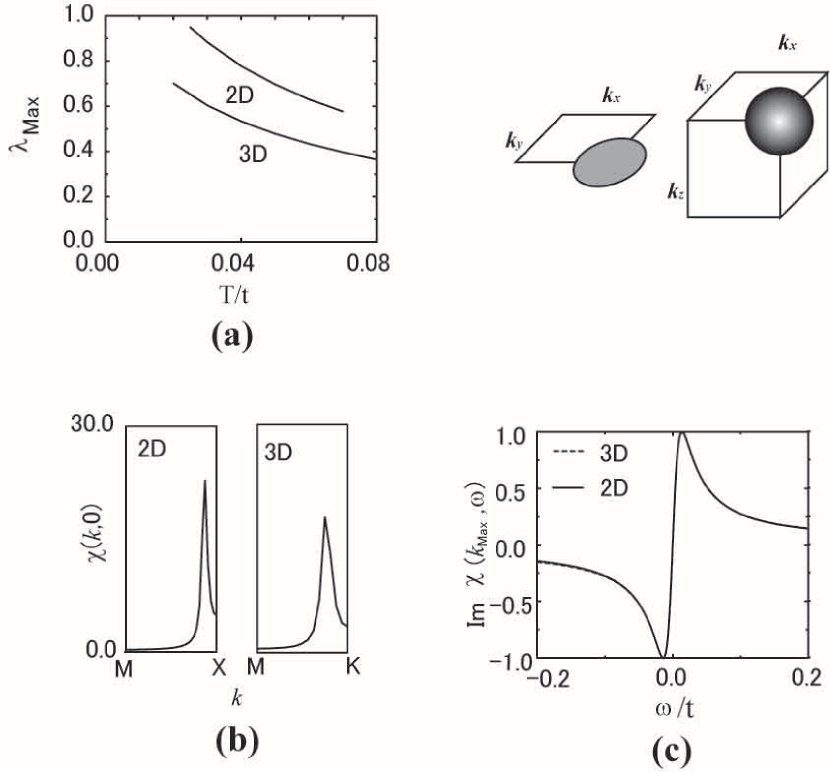
Figure 8: (a) The maximum eigenvalue of the Éliashberg equation against temperature for the Hubbard model on a square lattice with $n=0.85$ and $U=4$ and on a cubic lattice with $n=0.8$, the second-neighbour hopping $t^{\prime}=-0.2$ and $U=8$. $\chi(\mbox{\boldmath$k$},0)$ (b) as a function of wavenumber and ${\rm Im}\chi(\mbox{\boldmath$k$}_{\rm Max},\omega)$ (c) (normalised by its maximum) as a function of $\omega/t$ at $T=0.03t$ are also shown for the two lattices. Top right panel schematically shows the regions, in respective dimensions, that contribute to the pairing.

$T_{C}$ is identified as the temperature at which $\lambda_{\rm Max}$ becomes unity, which occurs at $T\sim 0.02$ for the square lattice, in accord with previous resultsDahm ; finitetc .

If we move on to the case with ferromagnetic spin fluctuations where triplet pairing is expected, this situation can be realised for relatively large $t^{\prime}(\simeq 0.5)$ and away from half-filling in the 2D Hubbard model. Physically, the van Hove singularity shifts toward the band bottom with $t^{\prime}$, and the large density of states at the Fermi level for the dilute case favours the ferromagnetism. We have found that $\lambda_{\rm Max}$ becomes largest for $n=0.3$, $t^{\prime}=0.5$.

$\chi_{\rm RPA}$ is indeed peaked at $\Gamma$ ($\mbox{\boldmath$k$}=(0,0)$). The question then is the behavior of $\lambda_{\rm Max}$ as a function of $T$, which shows that $\lambda_{\rm Max}$ is much smaller than that in the AF case.

A low $T_{C}$ for the ferromagnetic case contrasts with a naive expectation from the BCS picture, in which the Fermi level located around a peak in the density of states favours superconductivity. We may trace back two-fold reasons why this does not apply. First, if we look at the dominant ($\propto 1/[1-U\chi_{0}(q)]$) term of the pairing potential $V^{(2)}$ itself in eqs. (22) and (23), the triplet pairing interaction is only one-third of that for singlet pairing. Second, the factor $|G|^{2}$ for the ferromagnetic case is smaller than that in the AF case, which implies that the self-energy correction is larger in the former. Larger self-energy (smaller $|G|^{2}$) works unfavourably for superconductivity as seen in the Éliashberg equation (17). When we take a larger repulsion $U$ to increase the triplet pairing attraction (susceptibility), this makes the self-energy correction even stronger.

Let us now move on to the case of $d$-wave pairing in the 3D Hubbard model, for which FLEX was first applied by Arita et al2d3d . In simple-cubic systems, we find that the $\Gamma_{3}^{+}$ representation of O_h groupSigrist has the largest $\lambda_{\rm Max}$. We have found that $\lambda_{\rm Max}$ for this symmetry becomes largest for $n=0.8$, $t^{\prime}=-0.2\sim-0.3$ and $U=8\sim 10$. In Fig. 8(a), we superpose $\lambda_{\rm Max}$ as a function of $T$, where we can immediately see that the pairing tendency in 3D is much weaker than that in 2D.

Why is the $d$-superconductivity much stronger in 2D than in 3D? We can pinpoint the origin by looking at the various factors involved in the Éliashberg equation. Namely we question the height of $V^{(2)}$ and $|G|^{2}$ along with the width of the region, both in the momentum sector and in the frequency sector, over which $V^{(2)}(k)$ contributes to the summation over $k\equiv(\mbox{\boldmath$k$},i\omega_{n})$. We found that the maximum of $|G|^{2}$ is in fact larger in 3D than in 2D. The width of the peak in $\chi_{\rm RPA}$ on the frequency and momentum axes is surprisingly similar between 2D and 3D as displayed in Fig.8(b)(c). Note that if the frequency spread of the susceptibility scaled not with $t$ but with the band width, as Nakamura et alNakamura have assumed, $\lambda_{\rm Max}$ would have become larger. Now, $\lambda$ in the Éliashberg equation (17) is $\propto(a/L)^{D}$, where $L$ is the linear dimension of the system and $a$ the width in the momentum space for the effective attraction, this factor is much smaller in 3D than in 2D as far as the main contribution of $V^{(2)}$ to the pairing occurs through special points in the k-space (e.g., $(\pi,\pi)$ or $(\pi,\pi,\pi)$ for the antiferromagnetic spin fluctuation exchange pairing). So we can conclude that this is the main reason why 2D is more favourable than 3D.

To summarise this section, $d$-pairing in 2D is the best situation for the repulsion originated (i.e., spin fluctuation mediated) superconductivity in the Hubbard model. Monthoux and LonzarichMonLon have also concluded for 2D systems, by making use of a phenomenological approach, that the $d$-wave pairing is much stronger than $p$-wave pairing, which is consistent with the present result. In this sense, the layer-type cuprates do seem to hit upon the right situation.

This is as far as one-band model having simple Fermi surfaces are concerned. Indeed, if we turn to heavy fermion superconductors, for instance, in which the pairing is thought to be meditated by spin fluctuations, the $T_{C}$, when normalized by the band width $W$, is known to be of the order of $0.001W$. Since the present result indicates that $T_{C}$, normalized by $W$, is $\sim 0.0001W$ at best in the 3D Hubbard model, we may envisage that the heavy fermion system must exploit other factors such as the multiband. Neverthless, recent experimental findingrh that a heavy-fermion compound Ce(Rh,Ir,Co)In₅ has the higher $T_{c}$ for the more two-dimensional lattice (with larger $c/a$) is consistent with our prediction.

6 How to realise higher $T_{C}$ in anisotropic pairing — disconnected Fermi surfaces

Ironically, the main question about the superconductivity from the electronic mechanism is “why is $T_{C}$ so low?”, which has been repeatedly raised in literatures. Namely, one remarkable point is $T_{c}\sim O(0.01t)$, esitmated for the repulsive Hubbard model in the two-dimensional (2D) square lattice, is two orders of magnitudes smaller than the starting electronic energy (i.e., the hopping integral $t$), although this gives the right order for the curates’ $T_{c}$. We have seen that even the best case, as far as these ordinary lattices are concerned, has $T_{c}\sim O(0.01t)$. As discussed in Ref. Kuroki&Arita , there are good reasons why $T_{c}$ is so low: One reason is the effective attraction mediated by spin fluctuations is much weaker than the original electron-electron interaction, $U$. Another important reason is the presence of nodes in the superconducting gap function greatly reduces $T_{c}$: While the main pair-scattering, across which the gap function has opposite signs to make the effective interaction attractive, there are other pair scatterings around the nodes that have negative contributions to the effective attraction by connecting $k$-points on which the gap has the same sign.

So a next important avenue to explore is: can we improve the situation by going over to multiband systems. Kuroki and Arita Kuroki&Arita have shown that this is indeed the case if we have disconnected Fermi surfaces. In this case $T_{c}$ is dramatically enhanced, because the sign change in the gap function can avoid the Fermi pockets, where all the pair-scattering processes contribute positively. Kuroki&Arita ; NTT This has been numerically shown to be the case for the triangular lattice (for spin-triplet pairing) KAfortri and a squre lattice with a period-doubling Kuroki&Arita , where $T_{c}$ as estimated with FLEX is as high as $O(0.1t)$.

To be more precise, the key ingredients are: (a) when the Fermi surface is nested, the spin susceptibility $\chi(\mbox{\boldmath$q$},\omega)$ has a peak. (b) When a multiband system with a disconnected Fermi surface has an inter-pocket nesting (i.e., strong inter-pocket pair scattering and weak intra-pocket one) the gap function has the same sign ($s$-wave symmetry) within each pocket, and the nodal lines can happily run in between the pockets. The estimated $T_{c}$ for two-dimensional (2D) Hubbard model on such lattices is indeed almost an order of magnitude higher, $T_{c}\sim 0.1t$, as displayed in Fig.9 along with the lattice structure.

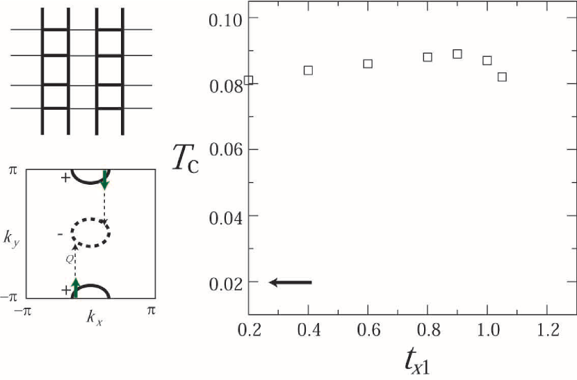
Figure 9: The $T_{C}$ estimated for the lattice depicted in the top left panel having disconnected Fermi surface (bottom left) as a function of the weak transfer (thin lines in the top left panel; $t_{x1}$).Kuroki&Arita The arrow indicates typical $T_{C}$ for ordinary (e.g., square) lattices.

As for the dimensionality of the system, we have shown above that 2D systems are generally more favourable than 3D systems as far as the spin-fluctuation-mediated superconductivity in ordinary lattices (square, triangular, fcc, bcc, etc) are concerned. Now, if one puts the idea for the disconnected Fermi surface on the above observation on the dimensionality, a natural question is: can we conceive 3D lattices having disconnected Fermi surfaces that have high $T_{c}$’s. More specifically, can the disconnected Fermi surface overcome the disadvantage of 3D? If we express our idea more explicitly, what we have in mind is the interband nesting (or Suhl-Kondo process in its broader context) in the 3D disconnected Fermi surface as depicted in Fig.10.

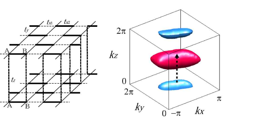
Figure 10: Interband nesting (arrow in the right panel) in 3D on a disconnected Fermi surface, which is exemplified here for the stacked bond-alternating lattice (left).

There, the nesting vector runs across the two bands, and this is envisaged to give the attractive pair-scattering interaction. So the gap function should be nodeless within each band, while the gap has opposite signs between the two bands.

In our most recent studyonari3d we have found that a stacked bond-alternating lattice (Fig.10) has a compact and disconnected (i.e., a pair of ball-like) Fermi pockets. We have shown that $T_{c}$ is $O(0.01t)$, which is the same order of that for the square lattice, and remarkably high for a 3D system. We have further found that the $T_{c}$ can be made even higher ($\sim O(0.1t))$ in a model in which the original Kuroki-Arita 2D system having disconnected Fermi surface is stacked. So the final message obtained here, starting from 1D and ending up with 3D, is that 3D material with considerably high $T_{c}$ can be expected if we consider appropriate lattice structures.

7 Closing remarks

So we have seen the electronic properties of electron systems with short-range repulsive interactions, starting from 1D up to 3D systems. While the quasi-1D ladders already contain seeds for the d-wave pairing, anisotropic pairing has more degrees of freedom in 2D and 3D where the topology (e.g., disconnected Fermi surfaces) of the Fermi surface can greatly favour higher Tc. Finally it would be needless to stress that the electron correlation is such a fascinating subject that there are many open questions to be explored. Among them, a question we can ask is what would happen to the superconductivity from the repulsive electron interaction when disorder is introduced in the system. Then we have a problem of dirty superconductors, i.e., an interplay of interaction and disorder. For ladders there are some discussions on this. For instance, Kimura et al.Kimuratransp have looked at the dirty double wire (i.e., two-band Tomonaga-Luttinger system with impurities), and noted that in the phases where the pairing correlation is dominant, the Anderson localisation is absent despite the system being quasi-1D. How this would be extended to higher dimensions is an interesting issue.

Acknowledgements — First and foremost, I wish to thank Professor Bernard Kramer for many years of interactions and discussions, dating back to the advent period when the Anderson localisation just began to form a main stream in the condensed matter physics. For the physics on Tomonaga-Luttinger and electron-mechanism superconductivity I would like to thank Kazuhiko Kuroki for collaboration. I also wish to acknowledge Ryotaro Arita, Takashi Kimura, Miko Eto, Michele Fabrizio and Seiichiro Onari for collaborations. Some of the works described here have been supported by Grants-in-aids from the Japanese Ministry of Education, and I also thank Yasumasa Kanada for a support in ‘Project for Vectorised Supercomputing’ in the numerical works.

References

- (1) W. Kohn and J.M. Luttinger, Phys. Rev. Lett. 15, 524 (1965).
- (2) D. Fay and A. Layzer: Phys. Rev. Lett. 20, 187 (1968); A. Layzer and D. Fay: Int. J. Magn. 1, 135 (1971).
- (3) The pairing for more dilute electron gas is shown to be s-wave, where the dynamical interaction becomes negative (see, Takada ).
- (4) S. Tomonaga: Prog. Theoret. Phys. 5, 544 (1950).
- (5) For reviews of the Tomonaga-Luttinger theory, see J. Sólyom: Adv. Phys. 28, 201 (1979); V.J. Emery in Highly Conducting One-Dimensional Solids, ed. by J.T. Devreese et al.(Plenum, New York, 1979), p.247.
- (6) D.C. Mattis: The Theory of Magnetism I (Springer-Verlag, Berlin, 1988).
- (7) A. Luther and V.J. Emery: Phys. Rev. Lett. 33, 589 (1974).
- (8) P.A. Lee: Phys. Rev. Lett. 34, 1247 (1975).
- (9) C.M. Varma and A. Zawadowski: Phys. Rev. B 32, 7399 (1985).
- (10) K. Penc and J. Sólyom: Phys. Rev. B 41, 704 (1990).
- (11) A.M. Finkel’stein and A.I. Larkin: Phys. Rev. B 47, 10461 (1993).
- (12) N. Nagaosa and T. Ogawa: Solid State Commun. 88, 295 (1993).
- (13) T. Kimura, K. Kuroki, H. Aoki and M. Eto: Phys. Rev. B 49, 16852 (1994); T. Kimura, K. Kuroki, and H. Aoki: ibid 53, 9572 (1996).
- (14) M. Sassetti, F. Napoli and B. Kramer: Phys. Rev. B 59, 7297 (1999).
- (15) H.J. Schulz: Phys. Rev. B 34, 6372 (1986).
- (16) F.D.M. Haldane: Phys. Lett. A 93, 464 (1993).
- (17) Y. Nishiyama, N. Hatano and M. Suzuki: J. Phys. Soc. Jpn 64, 1967 (1994).
- (18) E. Dagotto, J. Riera, and D.J. Scalapino: Phys. Rev. B 45, 5744 (1992).
- (19) T.M. Rice, S. Gopalan and M. Sigrist: Europhys. Lett. 23, 445 (1993); Physica B 199 & 200, 378 (1994).
- (20) P.W. Anderson: Science 235, 1196 (1987).
- (21) M. Uehara, T. Nagata, J. Akimitsu, H. Takahashi, N. Môri and K. Kinoshita: J. Phys. Soc. Jpn. 65, 2764 (1996).
- (22) A.M. Finkel’stein and A.I. Larkin: Phys. Rev. B 47, 10461 (1993).
- (23) L. Balents and M.P.A. Fisher: Phys. Rev. B 53, 12133 (1996).
- (24) M. Fabrizio: Phys. Rev. B 48, 15838 (1993).
- (25) M. Fabrizio, A. Parola and E. Tosatti: Phys. Rev. B 46, 3159 (1992).
- (26) N. Nagaosa and M. Oshikawa: J. Phys. Soc. Jpn. 65, 2241 (1996).
- (27) H.J. Schulz: Phys. Rev. B 53, R2959 (1996).
- (28) R.M. Noack, S.R. White and D.J. Scalapino: Phys. Rev. Lett. 73, 882 (1994).
- (29) R.M. Noack, S.R. White and D.J. Scalapino: Physica C 270, 281 (1996).
- (30) E. Dagotto, J. Riera and D.J. Scalapino: Phys. Rev. B 45, 5744 (1992).
- (31) M. Sigrist and K. Ueda: Rev. Mod. Phys. 63, 239 (1991).
- (32) D. Poilblanc, H. Tsunetsugu and T.M. Rice: Phys. Rev. B 50, 6511 (1994).
- (33) H. Tsunetsugu, M. Troyer and T.M. Rice: Phys. Rev. B 49, 16078 (1994); ibid. 51, 16456 (1995).
- (34) C.A. Hayward et al.: Phys. Rev. Lett. 75, 926 (1995); C.A. Hayward and D. Poilblanc: Phys. Rev. B 53, 11721 (1996).
- (35) K. Sano: J. Phys. Soc. Jpn. 65, 1146 (1996).
- (36) Multiband Tomonaga-Luttinger model that includes pair transfer between two bands [K.A. Muttalib and V.J. Emery, Phys. Rev. Lett. 57, 1370 (1986)] or charge-charge coupling between the chains [K. Kuroki and H. Aoki, Phys. Rev. Lett. 72, 2947 (1994)] has been studied.
- (37) H. Suhl, B.T. Mattis and L.R. Walker: Phys. Rev. Lett. 3, 552 (1959).
- (38) J. Kondo: Prog. Theor. Phys. 29, 1 (1963).
- (39) J.E. Hirsch: Phys. Rev. B 31, 4403 (1985).
- (40) M. Imada and Y. Hatsugai: J. Phys. Soc. Jpn. 58, 3572 (1989).
- (41) N. Furukawa and M. Imada: J. Phys. Soc. Jpn. 61, 3331 (1992).
- (42) S. Sorella, E. Tosatti, S. Baroni, R. Car and M. Parrinello: Int. J. Mod. Phys. B 1, 993 (1988).
- (43) S.R. White, D.J. Scalapino, R.L. Sugar, E.Y. Loh, J.E. Gubernatis and R.T. Scalettar: Phys. Rev. B 40, 506 (1991).
- (44) W. von der Linden, I. Morenstern and H. de Raedt: Phys. Rev. B 41, 4669 (1990).
- (45) R.M. Noack, S.R. White and D.J. Scalapino: Europhys. Lett. 30, 163 (1995); Physica C 270, 281 (1996).
- (46) Y. Asai: Phys. Rev. B 52, 10390 (1995).
- (47) K. Yamaji and Y. Shimoi: Physica C 222, 349 (1994); K. Yamaji, Y. Shimoi, and T. Yanagisawa: ibid 235-240, 2221 (1994).
- (48) K. Kuroki and H. Aoki: Phys. Rev. B 56, R14287 (1997); J. Phys. Soc. Jpn 67, 1533 (1998).
- (49) S. Sorella et al.: Int. J. Mod. Phys. B 1, 993 (1988); S.R. White et al.: Phys. Rev. B 40, 506 (1989); M. Imada and Y. Hatsugai: J. Phys. Soc. Jpn. 58, 3752 (1989).
- (50) Three-leg - ladder has also been examined by T.M. Rice, S. Haas, M. Sigrist and F.C. Zhang: Phys. Rev. B 56, 14655 (1997) with exact diagonalisation and mean-field approximation, and by S.R. White and D.J. Scalapino: Phys. Rev. B 57, 3031 (1998) with DMRG.
- (51) M. Azuma, Z. Hiroi, M. Takano, K. Ishida and Y. Kitaoka: Phys. Rev. Lett. 73, 3463 (1994).
- (52) K. Ishida, Y. Kitaoka, Y. Tokunaga, S. Matsumoto, K. Asayama, M. Azuma, Z. Hiroi and M. Takano: Phys. Rev. B 53, 2827 (1996).
- (53) K. Kojima, A. Karen, G.M. Luke, B. Nachumi, W.D. Wu, Y.J. Uemura, M. Azuma and M. Takano: Phys. Rev. Lett. 74, 2812 (1995).
- (54) Z. Hiroi and M. Takano: Nature 377, 41 (1995).
- (55) H. Mayaffre, P. Auban-Senzier, D. Jérome, D. Poilblanc, C. Bourbonnais, U. Ammerahl, G. Dhalenne, and A. Revcolevschi: Science 279, 345 (1998).
- (56) T. Kimura, K. Kuroki and H. Aoki: Phys. Rev. B 54, R9608 (1996).
- (57) T. Kimura, K. Kuroki and H. Aoki: J. Phys. Soc. Jpn. 66, 1599 (1997); 67, 1377 (1998).
- (58) E. Arrigoni: Phys. Lett. A 215, 91 (1996); Phys. Rev. Lett. 83 128 (1999); Phys. Rev. B 61 7909 (2000). See also, for the even-odd conjecture for the spin gap, U. Ledermann, K. Le Hur, and T.M. Rice, Phys. Rev. B 62, 16383 (2000); U. Ledermann, Phys. Rev. B 64, 235102 (2001).
- (59) H.J. Schulz in Correlated Fermions and Transport in Mesoscopic Systems, ed. by T. Martin, G. Montambaux and J.T.T. Van (Editions Frontieres, Gif-sur-Yvette, 1996), p. 81.
- (60) To be precise the CuO2 plane consists of a square array of Cu d orbitals and O p orbitals, which are usually modelled by the “d-p” model. Quantum Monte Carlo has indeed detected a long-ranged pairing correlation [K. Kuroki and H. Aoki: Phys. Rev. Lett. 76, 4400 (1996)]. The d-p model can be mapped to a one-band Hubbard model [see M.S. Hybertsen, E.B. Stechel, M. Schlüter, and D.R. Jennison: Phys. Rev. B 41, 11068 (1990); M.S. Hybertsen and M. Schlüter in New Horizons in Low-Dimensional Electron Systems ed. by H. Aoki et al (Kluwer, Dordrecht, 1992) p.229, and refs therein].
- (61) P.W. Anderson: A Carrier in Theoretical Physics (World Scientific, Singapore, 1994) and refs therein.
- (62) T. Moriya, Y. Takahashi, and K. Ueda: J. Phys. Soc. Jpn, 59, 2905 (1990); Physica C 185-189, 114 (1991).
- (63) T. Ueda, T. Moriya, and Y. Takahashi in Electronic Properties and Mechanisms of High- Superconductors ed. T. Oguchi et al. (North Holland, Amsterdam, 1992), p. 145; J. Phys. Chem. Solids 53, 1515 (1992).
- (64) T. Moriya and K. Ueda: J. Phys. Soc. Jpn. 63, 1871, (1994).
- (65) P. Monthoux, A. V. Balatsky, and D. Pines: Phys. Rev. B 46, 14803 (1992);
- (66) N.E. Bickers, D.J. Scalapino, and S.R. White: Phys. Rev. Lett. 62, 961 (1989).
- (67) I.E. Dzyaloshinskii: Zh.Eksp. Teor. Fiz. 93, 2267 (1987).
- (68) H.J. Schulz: Europhys. Lett. 4, 609 (1987).
- (69) D.J. Scalapino: Phys. Rep. 250, 329 (1995).
- (70) J.V. Alvarez, J. Gonzalez, F. Guinea and M.A.H. Vozmediano: J Phys. Soc. Jpn 67, 1868 (1998).
- (71) N. E. Bickers, D. J. Scalapino, and S. R. White: Phys. Rev. Lett. 62, 961 (1989); N. E. Bickers and D. J. Scalapino: Ann. Phys. (N. Y.) 193, 206 (1989).
- (72) T. Dahm and L. Tewordt: Phys. Rev. B 52, 1297 (1995).
- (73) J.J. Deisz, D. W. Hess, and J. W. Serene: Phys. Rev. Lett. 76, 1312 (1996).
- (74) E. Dagotto et al.: Phys. Rev. B 41, 811 (1990).
- (75) G. Fano, F. Ortolani, and A. Parola: Phys. Rev. B 42, 6877 (1990).
- (76) S.R. White et al.: Phys. Rev. B 39, 839 (1989); Phys. Rev. B 40, 506 (1989).
- (77) T. Husslein et al.: Phys. Rev. B 54, 16179 (1996).
- (78) S. Zhang, J. Carlson, and J.E. Gubernatis: Phys. Rev. Lett. 78, 4486 (1997).
- (79) T. Giamarchi and C. Lhuillier: Phys. Rev. B 43, 12943 (1991).
- (80) T. Nakanishi, K. Yamaji, and T. Yanagisawa: J. Phys. Soc. Jpn. 66 294 (1997).
- (81) N. Furukawa and M. Imada: J. Phys. Soc. Jpn. 61, 3331 (1992).
- (82) A. Moreo: Phys. Rev. B 45, 5059 (1992).
- (83) G. Sugiyama and S.E. Koonin: Ann. Phys. 168, 1 (1986); S. Sorella et al.: Int. J. Mod. Phys. B 1, 993 (1988); S.R. White et al.: Phys. Rev. B 40, 506 (1989); M. Imada and Y. Hatsugai: J. Phys. Soc. Jpn., 58, 3752 (1989).
- (84) K. Kuroki, T. Kimura, and H. Aoki: Phys. Rev. B 54, R15641 (1996).
- (85) P.A. Lee and N. Read: Phys. Rev. Lett. 58, 2691 (1987).
- (86) D.M. Newns et al.: Phys. Rev. Lett. 69, 1264 (1992).
- (87) R.S. Markiewicz et al.: Physica C 217, 381 (1993) and references therein.
- (88) J. Gonzalez and J.V. Alvarez: Phys. Rev. B 56, 367 (1997).
- (89) K. Kuroki and H. Aoki: Phys. Rev. B 60, 3060 (1999).
- (90) R. Arita, K. Kuroki and H. Aoki: Phys. Rev. B 60, 14585 (1999); J. Phys. Soc. Jpn. 69, 1181 (2000).
- (91) D. J. Scalapino, E. Loh, Jr., and J. E. Hirsh: Phys. Rev. B 34, 8190 (1986).
- (92) S. Nakamura, T. Moriya and K. Ueda: J. Phys. Soc. Jpn 65, 4026 (1996).
- (93) A. J. Leggett: Rev. Mod. Phys. 47, 331 (1975).
- (94) H. Tou et al.: Phys. Rev. Lett. 77, 1374 (1996); ibid, 80, 3129 (1998).
- (95) Y. Maeno et al.: Nature 372, 532 (1994); T. M. Rice, M. Sigrist: J. Phys. Condens. Matter 7, L643 (1995).
- (96) M.Y. Kagan and A.V. Chubukov: JETP Lett. 47, 614 (1988); A.V. Chubukov: Phys. Rev. B 48, 1097 (1993).
- (97) Y. Takada: Phys. Rev. B 47, 5202 (1993).
- (98) C. A. Kukkonen and A. W. Overhauser: Phys. Rev. B 20, 550 (1979).
- (99) A. V. Chubukov and J. P. Lu: Phys. Rev. B 46, 11163 (1992).
- (100) R. Hlubina: Phys. Rev. B 59, 9600 (1999).
- (101) H. Takahashi [J. Phys. Soc. Jpn, 68, 194 (1999)] on the other hand concludes that -wave channel is most attractive for dilute () 2D Hubbard model on the square lattice.
- (102) G. Baym and L.P. Kadanoff: Phys. Rev. 124, 287 (1961); G. Baym: Phys. Rev. 127, 1391 (1962).
- (103) Here a finite in 2D systems is thought of as a measure of when the layers are stacked to Josephson-couple.
- (104) P. Monthoux and G. G. Lonzarich: Phys. Rev. B 59, 14598 (1999).
- (105) P.G. Pagliuso, R. Movshovich, A.D. Bianchi, M. Nicklas, N.O. Moreno, J.D. Thompson, M.F. Hundley, J.L. Sarrao, Z. Fisk: Physica B 312, 129 (2002).
- (106) K. Kuroki, and R. Arita: Phys. Rev. B 64, 024501 (2001).
- (107) T. Kimura, H. Tamura, K. Kuroki, K. Shiraishi, H. Takayanagi, and R. Arita: Phys. Rev. B 68, 132508 (2002).
- (108) K. Kuroki and R. Arita: Phys. Rev. B 63, 174507 (2001).
- (109) S. Onari, K. Kuroki, R. Arita and H. Aoki: Phys. Rev. B 65, 184525 (2002); in preparation.
- (110) T. Kimura, K. Kuroki, and H. Aoki: Phys. Rev. B 51, 13860 (1995).