Critical equation of state of randomly dilute Ising systems

Abstract

We determine the critical equation of state of three-dimensional randomly dilute Ising systems, i.e. of the random-exchange Ising universality class. We first consider the small-magnetization expansion of the Helmholtz free energy in the high-temperature phase. Then, we apply a systematic approximation scheme of the equation of state in the whole critical regime, that is based on polynomial parametric representations matching the small-magnetization of the Helmholtz free energy and satisfying a global stationarity condition. These results allow us to estimate several universal amplitude ratios, such as the ratio $A^{+}/A^{-}$ of the specific-heat amplitudes. Our best estimate $A^{+}/A^{-}=1.6(3)$ is in good agreement with experimental results on dilute uniaxial antiferromagnets.

I Introduction.

The critical properties of randomly dilute Ising systems have been much investigated experimentally and theoretically, see, e.g., Refs. [1, 2, 3, 4, 5] for reviews. The typical example is the ferromagnetic random Ising model (RIM) with Hamiltonian

$${\cal H}=-J\sum_{<ij>}\rho_{i}\,\rho_{j}\;s_{i}s_{j}-H\sum_{i}\rho_{i}s_{i},$$ (1)

where $J>0$, the first sum extends over all nearest-neighbor sites, $s_{i}=\pm 1$ are Ising spin variables, and $\rho_{i}$ are uncorrelated quenched random variables, which are equal to one with probability $p$ (the spin concentration) and zero with probability $1-p$ (the impurity concentration). Considerable work has been dedicated to the identification of the universal critical behavior of the RIM, and in particular to the determination of the critical exponents, which have been computed with great accuracy in experiments and in theoretical works. On the other hand, much less is known about the critical equation of state and the corresponding universal amplitude ratios. From the experimental side, this is essentially due to the fact that typical experimental realizations of the RIM are uniaxial antiferromagnets such as Fe_xZn_1-xF₂ and Mn_xZn_1-xF₂ materials, which are usually modeled by the Hamiltonian (1) with $J<0$. For $H=0$, there is a simple mapping between the ferromagnetic and the antiferromagnetic model, so that the critical behavior of the antiferromagnets can still be obtained from that of the ferromagnetic RIM. The situation is more complex for $H\not=0$. The RIM (1) with $H\not=0$ corresponds to an antiferromagnet with a staggered magnetic field that cannot be realized experimentally. Conversely, antiferromagnets in a uniform magnetic field have a different critical behavior and belong to the same universality class of the ferromagnetic random-field Ising model [6]. For these reasons the equation of state of the RIM is not relevant for dilute uniaxial antiferromagnets. However, from the equation of state one can derive amplitude ratios involving quantities defined in the high- and low-temperature phase that can be measured experimentally, see, e.g., Ref. [3]. For example, the ratio $A^{+}/A^{-}$ of the specific-heat amplitudes in the high- and low-temperature phase has been determined: $A^{+}/A^{-}=1.6(3)$ (Ref. [7]), and $A^{+}/A^{-}=1.55(15)$ (Ref. [3]). On the theoretical side, only a few works, based on field-theoretical (FT) perturbative expansions, have attempted to determine other universal quantities beside the critical exponents [8, 9, 10, 11, 12], obtaining rather imprecise results. For example, these calculation have not even been able to determine reliably the sign of the ratio $A^{+}/A^{-}$. Actually, $\epsilon$-expansion calculations [9, 10] favor a negative value, in clear disagreement with experiments.

In this paper we determine the equation of state of the RIM in the critical region, that is the relation among the external field $H$, the reduced temperature $t\equiv(T-T_{c})/T_{c}$, and the magnetization

$$M\equiv{1\over V}\overline{\langle\sum_{i}\rho_{i}s_{i}\rangle},$$ (2)

where the overline indicates the average over the random variables $\rho_{i}$, and $\langle\;\;\rangle$ indicates the sample average at fixed disorder. It can be written in the usual form as

$$H\propto M^{\delta}f(x),\qquad x\propto tM^{1/\beta},$$ (3)

where $x$ and $f(x)$ are normalized so that $x=-1$ corresponds to the coexistence curve, hence $f(-1)=0$, and $f(0)=1$. In order to determine the critical equation of state in the whole critical region, we use an approximation scheme that has already been applied with success to the pure Ising model in three [13, 14, 15] and in two dimensions [16]. We first consider the expansion of the equation of state in terms of the magnetization in the high-temperature phase. The first few nontrivial coefficients can be determined either from Monte Carlo simulations of the RIM or from the analysis of FT perturbative expansions. These results are then used to construct approximations that are valid in the whole critical region and that allow us to determine several universal amplitude ratios. For example, we anticipate our best estimate of the specific-heat amplitude ratio

$$A^{+}/A^{-}=1.6(3),$$ (4)

which compares very well with the experimental determinations in dilute uniaxial antiferromagnets [7, 3].

The paper is organized as follows. In Sec. II we discuss the general properties of the critical equation of state. In Sec. III we consider its small-magnetization expansion in the high-temperature phase, reporting estimates of the first few nontrivial terms, obtained by Monte Carlo simulations and FT methods. These results are used in Sec. IV to construct approximate polynomial parametric representations that are valid in the whole critical region and that allow us to achieve a rather accurate determination of the scaling function $f(x)$. Finally, in Sec. V we determine several universal amplitude ratios, such as the specific-heat amplitude ratio $A^{+}/A^{-}$. In App. A we report the definitions of the thermodynamic quantities that are considered in the paper. In App. B we discuss the correspondence between the RIM correlation functions and the correlation functions of the corresponding translation-invariant field theory that is obtained by using the standard replica trick. App. C reports some details on the six-loop FT calculation of the universal amplitude ratio $R_{\xi}^{+}$.

II The critical equation of state

The equation of state relates the magnetization $M$, the magnetic field $H$, and the reduced temperature $t\equiv(T-T_{c})/T_{c}$. In the neighborhood of the critical point $t=0$, $H=0$, it can be written in the scaling form

$$H=B_{c}^{-\delta}M^{\delta}f(x),$$ (5)

$$x\equiv t(M/B)^{-1/\beta},$$ (6)

where $B_{c}$ and $B$ are the amplitudes of the magnetization on the critical isotherm and on the coexistence curve, see App. A. According to these normalizations, the coexistence curve corresponds to $x=-1$, and the universal function $f(x)$ satisfies $f(-1)=0$ and $f(0)=1$. The apparently most precise estimates of the critical exponents have been recently obtained by Monte Carlo simulations of the RIM: Ref. [17] obtains $\nu=0.683(3)$ and $\eta=0.035(2)$, while Ref. [18] reports $\nu=0.6837(53)$ and $\eta=0.0374(45)$. The FT estimates $\nu=0.678(10)$ and $\eta=0.030(3)$, obtained by analyzing six-loop fixed-dimension series [19], are in good agreement [20]. The other exponents $\alpha$, $\gamma$, $\beta$, and $\delta$ can be determined using scaling and hyperscaling relations.

The equation of state is analytic for $|H|>0$, implying that $f(x)$ is regular everywhere for $x>-1$. In particular, $f(x)$ has a regular expansion in powers of $x$ around $x=0$

$$f(x)=1+\sum_{n=1}^{\infty}f_{n}^{0}x^{n}.$$ (7)

At the coexistence curve, i.e., for $x\rightarrow-1$, $f(x)$ is expected to have an essential singularity [21], so that it can be asymptotically expanded as

$$f(x)\approx\sum_{n=1}^{\infty}f^{\rm coex}_{n}(1+x)^{n}.$$ (8)

The free energy of a dilute ferromagnet is nonanalytic at $H=0$ for all temperatures below the transition temperature of the pure system [22], which is larger than the critical temperature of the dilute one. Therefore, at variance with pure systems, the equation of state of the RIM is also nonanalytic for $t>0$ and $H=0$. However, as argued in Ref. [23], these singularities are very weak and all derivatives remain finite at $H=0$, as it happens at the coexistence curve. This allows us to write down an asymptotic large-$x$ expansion of the form

$$f(x)=x^{\gamma}\sum_{n=0}^{\infty}f_{n}^{\infty}x^{-2n\beta}.$$ (9)

It is useful to rewrite the equation of state in terms of a variable proportional to $Mt^{-\beta}$, although in this case we must distinguish between $t>0$ and $t<0$. For $t>0$ we define

$$H=\left({C^{+}\over C_{4}^{+}}\right)^{1/2}t^{\beta\delta}F(z),$$ (10)

$$z\equiv\left[-{C_{4}^{+}\over(C^{+})^{3}}\right]^{1/2}Mt^{-\beta},$$ (11)

while for $t<0$ we set

$$H={B\over C^{-}}(-t)^{\beta\delta}\Phi(u),$$ (12)

$$u\equiv{M\over B}(-t)^{-\beta}.$$ (13)

The constants $C^{\pm}$ and $C^{+}_{4}$ are the amplitudes appearing in the critical behavior of the two- and four-point susceptibilities $\chi$ and $\chi_{4}$ respectively, see App. A. With the chosen normalizations [4],

$$F(z) = z+{1\over 6}z^{3}+\sum_{j=3}{1\over(2j-1)!}r_{2j}\,z^{2j-1},$$ (14)

$$\Phi(u) = (u-1)+\sum_{j=3}^{\infty}{1\over(j-1)!}v_{j}\,(u-1)^{j-1}.$$ (15)

The large-$z$ expansion of the scaling function $F(z)$ is given by

$$F(z)=z^{\delta}\sum_{k=0}F^{\infty}_{k}z^{-k/\beta}.$$ (16)

The functions $F(z)$ and $\Phi(u)$ are clearly related to $f(x)$. Indeed,

$$z^{-\delta}F(z)=F_{0}^{\infty}f(x),\qquad\qquad z=z_{0}x^{-\beta},$$ (17)

$$u^{-\delta}\Phi(u)={C^{-}B^{\delta-1}\over B_{c}^{\delta}}f(x),\qquad u=(-x)^{-\beta}.$$ (18)

where $z_{0}=(R_{4}^{+})^{1/2}$ is a universal constant, see Sec. V.

In order to determine the critical equation of state, we first consider its small-magnetization expansion. Then, we construct parametric representations of the critical equation of state based on polynomial approximations, which are valid in the whole critical region. This method have already been applied to the Ising universality class in three [13, 14, 15] and two dimensions [16], and to the three-dimensional $XY$ and Heisenberg universality classes [24, 25].

III Small-magnetization expansion in the high-temperature phase

A Small-magnetization expansion of the Helmholtz free energy

In the high-temperature phase the quenched Helmholtz free energy ${\cal A}(t,M)$ admits an expansion around $M=0$:

$$\xi^{3}\left[{\cal A}(t,M)-{\cal A}(t,0)\right]={1\over 2}\hat{M}^{2}+\sum_{j=2}{1\over(2j)!}G_{2j}\hat{M}^{2j},$$ (19)

where $\xi$ is the second-moment correlation length along the axis $H=M=0$, $\hat{M}\equiv cM\xi^{\beta/\nu}$, $c\equiv(f^{+})^{1-\eta/2}/(C^{+})^{1/2}$, and $C^{+}$, $f^{+}$ are the amplitudes of $\chi$ and $\xi$ respectively, see App. A for notations. We recall that the equation of state is related to the Helmholtz free energy by

$$H={\partial{\cal A}(t,M)\over\partial M},$$ (20)

and therefore the expansion (19) is strictly related to the expansion of the function $F(z)$, cf. Eq. (11).

In the critical limit the coefficients $G_{2j}$ of the expansion (19) are universal. They can be determined from the high-temperature critical limit of combinations of zero-momentum connected correlation functions averaged over the random dilution

$$\chi_{n}=\left.{\partial^{n-1}M\over\partial H^{n-1}}\right|_{H=0}\;.$$ (21)

Indeed,

$$G_{4}=\lim_{t\rightarrow 0^{+}}\;\lim_{V\rightarrow\infty}\;\left(-{\chi_{4}\over\xi^{d}\chi_{2}^{\,2}}\right),$$ (22)

$$G_{6}=\lim_{t\rightarrow 0^{+}}\;\lim_{V\rightarrow\infty}\;\left(-{\chi_{6}\over\xi^{2d}\chi_{2}^{\,3}}+{\chi_{4}^{\,2}\over\xi^{2d}\chi_{2}^{\,4}}\right),$$ (23)

$$G_{8}=\lim_{t\rightarrow 0^{+}}\;\lim_{V\rightarrow\infty}\;\left(-{\chi_{8}\over\xi^{3d}\chi_{2}^{\,4}}+56{\chi_{6}\chi_{4}\over\xi^{3d}\chi_{2}^{\,5}}-280{\chi_{4}^{\,3}\over\xi^{3d}\chi_{2}^{\,6}}\right),$$ (24)

where $\chi_{2}\equiv\chi$ and $V$ is the volume.

For the purpose of determining the small-magnetization expansion of the RIM equation of state, it is convenient to rewrite the Helmholtz free energy of the RIM, cf. Eq. (19), in the equivalent form

$${\cal A}(t,M)-{\cal A}(t,0)=-{(C^{+})^{2}\over C_{4}^{+}}t^{3\nu}A(z),$$ (25)

where $z$ is defined in Eq. (11),

$$A(z)={1\over 2}z^{2}+{1\over 4!}z^{4}+\sum_{j=3}{1\over(2j)!}r_{2j}z^{2j},$$ (26)

and

$$r_{2j}={G_{2j}\over G_{4}^{j-1}}\qquad\qquad j\geq 3.$$ (27)

Since $F(z)={dA(z)/dz}$, Eq. (11) follows from Eq. (26).

Some of these universal constants have been recently estimated by means of a Monte Carlo simulation [17], obtaining

$$G_{4}=43.3(2),\qquad r_{6}=0.90(15).$$ (28)

Correspondingly, $G_{6}=1.7(3)\times 10^{3}$.

B Field-theoretical approach

One may estimate the universal quantities $G_{2j}$ and $r_{2j}$ by FT methods. The FT approach is based on an effective Landau-Ginzburg-Wilson Hamiltonian [26] that can be obtained by using the replica method,

$${\cal H}_{\varphi^{4}}=\int d^{3}x\left\{{1\over 2}\sum_{i=1}^{N}\left[(\partial_{\mu}\varphi_{i})^{2}+r\varphi_{i}^{2}\right]+{1\over 4!}\sum_{i,j=1}^{N}\left(u_{0}+v_{0}\delta_{ij}\right)+H\sum_{i=1}^{N}\varphi_{i}\right\}\;,$$ (29)

where $\varphi_{i}$ is an $N$-component field. The critical behavior of the RIM is expected to be described by the Hamiltonian ${\cal H}_{\varphi^{4}}$ for $u_{0}<0$ and in the limit $N\rightarrow 0$. Conventional FT computational schemes show that the fixed point corresponding to the pure Ising model is unstable and that the renormalization-group flow moves towards another stable fixed point describing the critical behavior of the RIM.

The most precise FT results for the critical exponents have been obtained in the framework of the perturbative fixed-dimension expansion in terms of zero-momentum couplings. The corresponding Callan-Symanzik $\beta$-functions and the renormalization-group functions associated with the critical exponents have been computed to six loops [19, 27].

The Helmholtz free energy ${\cal A}_{\varphi^{4}}$ associated with the Hamiltonian (29) can be written as [28, 29]

$$\xi^{3}\left[{\cal A}_{\varphi^{4}}(M)-{\cal A}_{\varphi^{4}}(0)\right]={1\over 2}\sum_{a}\hat{M}_{a}^{2}+{1\over 4!}\sum_{ab}(g_{41}+g_{42}\delta_{ab})\hat{M}_{a}^{2}\hat{M}_{b}^{2}+$$ (30)

$$+{1\over 6!}\sum_{abc}(g_{61}+g_{62}\delta_{ab}+g_{63}\delta_{abc})\hat{M}_{a}^{2}\hat{M}_{b}^{2}\hat{M}_{c}^{2}+$$ (31)

$$+{1\over 8!}\sum_{abcd}\left(g_{81}+g_{82}\delta_{ab}+g_{83}\delta_{ab}\delta_{cd}+g_{84}\delta_{abc}+g_{85}\delta_{abcd}\right)\hat{M}_{a}^{2}\hat{M}_{b}^{2}\hat{M}_{c}^{2}\hat{M}_{d}^{2}+...$$ (32)

where $\hat{M}_{a}=cM_{a}\xi^{\beta/\nu}$, $c=\xi^{1-\eta/2}/\chi^{1/2}|_{H=0}$. Note that $g_{41}=u^{*}$ and $g_{42}=v^{*}$, where $u^{*}$ and $v^{*}$ are the fixed-point values of the renormalized quartic couplings $u$ and $v$. Applying the replica method in the presence of a uniform external field $H$, see App. B for details, one can identify

$$G_{4}=g_{42}=v^{*},\qquad G_{6}=g_{63},\qquad G_{8}=g_{85},$$ (33)

etc… It is worth noting that the other coefficients appearing in the small-magnetization expansion of the Helmholtz free energy (30), i.e. $g_{41}$, $g_{61}$, $g_{62}$, etc…, can be related to dilution averages of products of single-sample $n$-point correlation functions, as shown in App. B.

The quartic coupling $G_{4}$ can be estimated from the position of the RIM fixed point in the $u$, $v$ plane, i.e. from the common zero of their $\beta$-functions. The analysis of the six-loop perturbative series gives results somewhat dependent on the resummation method [19], see also the five-loop analysis of Ref. [30]. Combining all results together, one finds $36.5\lesssim G_{4}\lesssim 39.5$, which can be summarized as $G_{4}=38.0(1.5)$. Such a result is not consistent with the Monte Carlo estimate (28), obtained by estimating the limit given in Eq. (22). But, as discussed in Ref. [17], the quantitative consequences for the determination of the critical exponents are very small, since the renormalization-group functions corresponding to the critical exponents turn out to be little sensitive to the correct position of the fixed point [31] (along the Ising-to-RIM renormalization-group trajectory, see also Ref. [32]).

The universal constants $G_{6}$ and $r_{6}=G_{6}/G_{4}^{2}$ have been estimated in Ref. [29] by analyzing the corresponding four-loop series with the Padé-Borel method. These analyses provide the estimate $r_{6}\approx 1.09$. We have reanalyzed this series, finding that, unlike critical exponents, $r_{6}$ is rather sensitive to the position of the fixed point. Using the Monte Carlo estimates of $u^{*}$ and $v^{*}$ and the Padé-Borel method, we obtain $r_{6}\approx 0.6$. Thus, a conservative estimate is $r_{6}=1.1^{+0.1}_{-0.5}$, which is in agreement with the Monte Carlo result of Ref. [17] mentioned in Sec. III A, $r_{6}=0.90(15)$. We have also computed the fixed-dimension perturbative expansion of $r_{8}\equiv G_{8}/G_{4}^{3}$ to three loops. This requires the computation of the 8-point one-particle irreducible zero-momentum correlation function. At three loops this calculation requires the evaluation of 42 Feynman diagrams. For this purpose we have used the general algorithm of Ref. [33]. The expansion of $r_{8}$ is

$$r_{8}=-{105\over 64\pi}(8u+3v)+{35\over 9216\pi^{2}}(2480u^{2}+2286uv+585v^{2})$$ (34)

$$\;\;-0.132874\,u^{3}-0.199366\,u^{2}v-0.1080052\,uv^{2}-0.0211475\,v^{3}+...$$ (35)

where the zero-momentum quartic couplings $u$ and $v$ are normalized so that $u=u_{0}/m$ and $v=v_{0}/m$ at tree level (see App. C for precise definitions). We have checked that Eq. (34) correctly reproduces the known series for the O($N$) models [34] with $N=0,1$ in the appropriate limits. Unfortunately, the analysis of the expansion (34) provides only a very rough estimate [35], $r_{8}=15(15)$. We will obtain a much better estimate of $r_{8}$ in Sec. IV B, from the results for the equation of state.

IV Approximate representations of the critical equation of state

A Polynomial parametric representations

In order to obtain approximate expressions for the equation of state, we parametrize the thermodynamic variables in terms of two parameters $R$ and $\theta$, implementing all expected scaling and analytic properties. Explicitly, we write [36]

$$M = m_{0}R^{\beta}\theta,$$ (36)

$$t = R(1-\theta^{2}),$$ (37)

$$H = h_{0}R^{\beta\delta}h(\theta),$$ (38)

where $h_{0}$ and $m_{0}$ are normalization constants. The variable $R$ is nonnegative and measures the distance from the critical point in the $(t,H)$ plane; the critical behavior is obtained for $R\to 0$. The variable $\theta$ parametrizes the displacements along the lines of constant $R$. The line $\theta=0$ corresponds to the high-temperature phase $t>0$ and $H=0$; the line $\theta=1$ to the critical isotherm $t=0$; $\theta=\theta_{0}$, where $\theta_{0}$ is the smallest positive zero of $h(\theta)$, to the coexistence curve $T<T_{c}$ and $H\to 0$. Of course, one should have $\theta_{0}>1$ and $h(\theta)>0$ for $0<\theta<\theta_{0}$. The function $h(\theta)$ must be analytic in the physical interval $0\leq\theta<\theta_{0}$ in order to satisfy the requirements of regularity of the equation of state (Griffiths’ analyticity). Note that the mapping (38) is not invertible when its Jacobian vanishes [4], which occurs for $\theta^{2}_{l}=1/(1-2\beta)$. Thus, a parametric representation is acceptable only if $\theta_{0}<\theta_{l}$. The function $h(\theta)$ must be odd in $\theta$, to guarantee that the equation of state has an expansion in odd powers of $|M|$ in the high-temperature phase for $|M|\to 0$. Moreover, it can be normalized so that $h(\theta)=\theta+O(\theta^{3})$.

The scaling functions $f(x)$ and $F(z)$ can be expressed in terms of $\theta$. The scaling function $f(x)$ is obtained from

$$x={1-\theta^{2}\over\theta_{0}^{2}-1}\left({\theta_{0}\over\theta}\right)^{1/\beta},$$ (39)

$$f(x)=\theta^{-\delta}{h(\theta)\over h(1)},$$ (40)

while $F(z)$ is obtained by

$$z=\rho\theta\left(1-\theta^{2}\right)^{-\beta},$$ (41)

$$F(z(\theta))=\rho\left(1-\theta^{2}\right)^{-\beta\delta}h(\theta),$$ (42)

where $\rho$ can be related to $m_{0}$, $h_{0}$, $C^{+}$, and $C_{4}^{+}$ by using Eqs. (11) and (38).

Eq. (38) and the normalization condition $h(\theta)\approx\theta$ for $\theta\to 0$ do not completely fix the function $h(\theta)$. Indeed, one can rewrite the relation between $x$ and $\theta$ in the form

$$x^{\gamma}=h(1)\,f_{0}^{\infty}(1-\theta^{2})^{\gamma}\theta^{1-\delta}.$$ (43)

Thus, given $f(x)$, the value of $h(1)$ can be arbitrarily chosen to completely fix $h(\theta)$. One may fix this arbitrariness by choosing arbitrarily the parameter $\rho$ in the expression (42).

We approximate $h(\theta)$ with polynomials, i.e., we set

$$h(\theta)=\theta+\sum_{n=1}^{k}h_{2n+1}\theta^{2n+1}.$$ (44)

This approximation scheme turned out to be effective in the case of pure Ising systems [13, 14]. If we require the approximate parametric representation to give the correct $(k-1)$ universal ratios $r_{6}$, $r_{8}$, $\ldots$, $r_{2k+2}$, we obtain

$$h_{2n+1}=\sum_{m=0}^{n}c_{nm}6^{m}(h_{3}+\gamma)^{m}{r_{2m+2}\over(2m+1)!},$$ (45)

where

$$c_{nm}={1\over(n-m)!}\prod_{k=1}^{n-m}(2\beta m-\gamma+k-1),$$ (46)

and we have set $r_{2}=r_{4}=1$. Moreover, by requiring that $F(z)=z+{1\over 6}z^{3}+...$, we obtain the relation

$$\rho^{2}=6(h_{3}+\gamma).$$ (47)

In the exact parametric representation, the coefficient $h_{3}$ can be chosen arbitrarily. This is no longer true when we use our truncated function $h(\theta)$, and the related approximate function $f_{\rm approx}^{(k)}(x,h_{3})$ depends on $h_{3}$. We must thus fix a particular value for this parameter. In order to optimize this choice, we employ a variational procedure [14], requiring the approximate function $f_{\rm approx}^{(k)}(x,h_{3})$ to have the smallest possible dependence on $h_{3}$. This is achieved by setting $h_{3}=h_{3,k}$, where $h_{3,k}$ is a solution of the global stationarity condition

$$\left.{\partial f_{\rm approx}^{(k)}(x,h_{3})\over\partial h_{3}}\right|_{h_{3}=h_{3,k}}=0$$ (48)

for all $x$. The existence of such a value of $h_{3,k}$ for each $k$ is a nontrivial mathematical result which was proved in Ref. [14]. This procedure represents a systematic approximation scheme, which is only limited by the number of known terms in the small-magnetization expansion of the Helmholtz free energy. Note, for $k=1$, the so-called linear model, Eq. (48) gives

$$h_{3}={\gamma(1-2\beta)\over\gamma-2\beta},$$ (49)

which was considered as the optimal value of $h_{3}$ for the Ising equation of state [37].

B Results

TABLE I.: Expansion coefficients for the scaling equation of state obtained by the $k=1,2$ approximations of the parametric function $h(\theta)$. See text for definitions. The number marked with an asterisk is an input, not a prediction.

	$k=1$	$k=2$	Ising (Ref. [15])
$f^{0}_{1}$	1.100(2)	1.06(2)	1.0527(7)
$f^{0}_{2}$	0.083(1)	0.06(2)	0.0446(4)
$f^{0}_{3}$	$-$0.012(2)	$-$0.006(3)	$-$0.0059(2)
$f_{1}^{\rm coex}$	0.87(1)	0.93(8)	0.9357(11)
$f^{\infty}_{0}$	0.550(3)	0.48(3)	0.6024(15)
$r_{6}$	1.46(6)	∗0.90(15)	2.056(5)
$r_{8}$	1.0(3)	1.5(3)	2.3(1)
$v_{3}$	6.9(2)	6.3(2)	6.050(13)
$v_{4}$	17(1)	18.7(5)	16.17(10)
$F^{\infty}_{0}$	0.0235(6)	0.018(2)	0.03382(15)

We apply the method outlined in the preceding section, using the Monte Carlo estimates [17] $\nu=0.683(3)$, $\eta=0.035(2)$, $r_{6}=0.90(15)$ as input parameters. We obtain two different approximations corresponding to $k=1$ and $k=2$. Using the central values of the input parameters, we have

$$h(\theta)^{(k=1)}=\theta\left(1-\theta^{2}/\theta_{0}^{2}\right),\qquad\theta_{0}^{2}=1.61451,$$ (50)

that provides the optimal linear model, and

$$h(\theta)^{(k=2)}=\theta\left(1-\theta^{2}/\theta_{0}^{2}\right)\left(1+c_{1}\theta^{2}\right),$$ (51)

$$\theta_{0}^{2}=1.32141,\qquad c_{1}=0.106612.$$ (52)

The relatively small value of $c_{1}$ supports the effectiveness of the approximation scheme. In Table I we report results concerning the behavior of the scaling function $f(x)$, $F(z)$, and $\Phi(u)$ for $H=0$ and on the critical isotherm, cf. Eqs. (7), (8), (9), (14), (15), (16). The errors reported there are only related to the uncertainty on the corresponding input parameters. We consider the $k=2$ results as our best estimates. Of course, the corresponding errors do not take into account the systematic error due to the approximation scheme. Nevertheless, on the basis of the preceding applications [14, 15, 16] to the three- and two-dimensional Ising universality class, we believe that the $k=2$ approximation already provides a reliable estimate, and that one may take the difference with the $k=1$ result as indicative estimate of (or bound on) the systematic error. For comparison, the last column reports the corresponding estimates for the Ising universality class, taken from Ref. [15]. In Fig. 1 we show the scaling function $f(x)$, as obtained from the $k=1,2$ approximations of $h(\theta)$, using the central values of the input parameters. The difference between the two curves is rather small in the region $-1\leq x\lesssim 1$. For larger values of $x$ some differences are observed: they are essentially due to the small difference (approximately 10%) in the corresponding values of $f_{0}^{\infty}$.

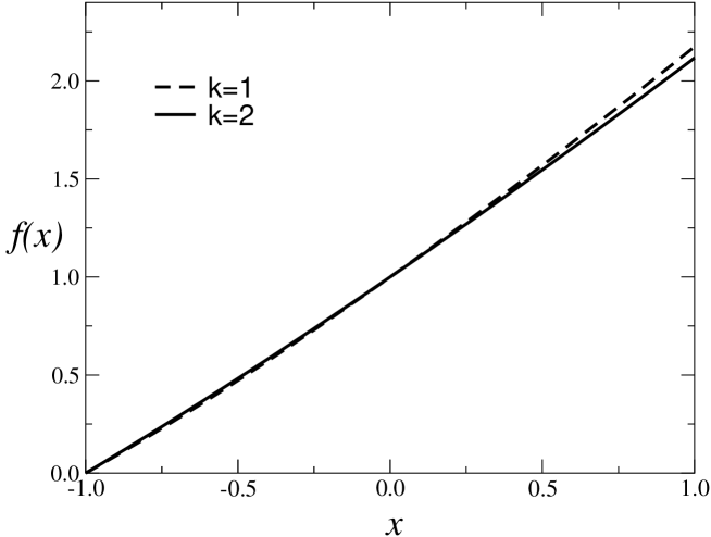
FIG. 1.: The scaling function $f(x)$.

V Universal amplitude ratios

Universal amplitude ratios characterize the critical behavior of thermodynamic quantities that do not depend on the normalizations of the external (magnetic) field, of the order parameter (magnetization), and of the temperature. From the scaling function $f(x)$ one may derive many universal amplitude ratios involving quantities defined at zero momentum (i.e. integrated in the volume), such as the specific heat, the magnetic susceptibility, etc…. For example, one can obtain estimates for the specific-heat amplitude ratio $A^{+}/A^{-}$, the sueceptibility amplitude ratio $C^{+}/C^{-}$, etc…. Then, using the results for $G_{4}$ and the relation

$$G_{4}\equiv-{C_{4}^{+}\over(C^{+})^{2}(f^{+})^{3}},$$ (53)

where $C_{4}^{+}$, $C^{+}$, and $f^{+}$ are respectively the amplitudes of the zero-momentum connected four-point correlation, the susceptibility, and the second-moment correlation length (see App. A for notations), we can also determine universal ratios involving the correlation-length amplitude $f^{+}$.

In Table II we report estimates of several amplitude ratios, as derived by using the approximate polynomial representations of the equation of state for $k=1,2$. Again, the errors reported there are only related to the uncertainty on the corresponding input parameters. Note that, in the most important case of $A^{+}/A^{-}$, the $k=2$ estimate includes the $k=1$ result within its error. As discussed in Sec. IV B, we consider the $k=2$ result as our best estimate for each quantity. As an indicative estimate of the total uncertainty, we take the maximum between the error induced by the input parameters and the difference with the $k=1$ result. This would lead to the final estimates $A^{+}/A^{-}=1.6(3)$, $C^{+}/C^{-}=5.5(1.0)$, $R_{c}^{+}=0.08(3)$, $R_{4}^{+}=12(2)$, $R_{\chi}=2.1(3)$ and $G_{4}^{1/3}R_{\xi}^{+}=0.99(1)$.

Universal amplitude ratios involving the correlation-length amplitude $f^{+}$, such as

$$R_{\xi}^{+}\equiv(\alpha A^{+})^{1/3}f^{+},\qquad Q_{c}\equiv B^{2}(f^{+})^{3}/C^{+},$$ (54)

can be obtained by using the Monte Carlo estimate of Ref. [17], $G_{4}=43.3(2)$:

$$R_{\xi}^{+}=\left({R_{4}^{+}R_{c}^{+}\over G_{4}}\right)^{1/3}=0.282(3),$$ (55)

$$Q_{c}={R_{4}^{+}\over G_{4}}=0.28(5).$$ (56)

TABLE II.: Universal amplitude ratios obtained from the $k=1,2$ approximations of the parametric function $h(\theta)$. Amplitude definitions are reported in App. A. For comparison, the last column reports the corresponding estimates for the Ising universality class, taken from Ref. [15].

	$k=1$	$k=2$	Ising
$A^{+}/A^{-}$	1.33(8)	1.58(26)	0.532(3)
$C^{+}/C^{-}$	4.5(2)	5.5(5)	4.76(2)
$R_{c}^{+}\equiv\alpha A^{+}C^{+}/B^{2}$	0.1008(5)	0.079(6)	0.0567(3)
$R_{4}^{+}\equiv-C_{4}^{+}B^{2}/(C^{+})^{3}$	9.9(2)	12.2(8)	7.81(2)
$R_{\chi}\equiv C^{+}B^{\delta-1}/(B_{c})^{\delta}$	1.82(1)	2.1(1)	1.660(4)
$G_{4}^{1/3}R_{\xi}^{+}\equiv(-\alpha A^{+}C_{4}^{+}/(C^{+})^{2})^{1/3}$	0.999(5)	0.989(5)	0.443(2)

The result for $R_{\xi}^{+}$ is in substantial agreement with the rather precise Monte Carlo estimate [17] $R_{\xi}^{+}=0.2885(15)$, providing support to our approximation of the equation of state. We have also obtained another independent estimate of the ratio $R_{\xi}^{+}$ by using the FT fixed-dimension approach in terms of zero-momentum renormalized coulings. As discussed in detail in App. C we have extended the five-loop calculation of Ref. [12] to six loops. The analysis of the perturbative expansions gives the estimate $R_{\xi}^{+}=0.290(10)$, which is in good agreement with the results from the equation of state and from Monte Carlo simulations.

The comparison with experiments on uniaxial antiferromagnets, see, e.g., Ref. [3] for a review, is essentially restricted to the specific-heat ratio $A^{+}/A^{-}$. Our best estimate $A^{+}/A^{-}=1.6(3)$ is in good agreement with the experimental result $A^{+}/A^{-}=1.6(3)$ reported in Ref. [7], and $A^{+}/A^{-}=1.55(15)$ reported in Ref. [3]. Earlier FT studies in the framework of $\epsilon$ and fixed-dimension expansions [9, 10, 11] provided rather imprecise results. Actually, they favored a negative value, in substantial disagreement with experiments.

Other experimental results concern the staggered magnetic susceptibility and the correlation length, see, e.g., Refs. [38, 3], which are determined from neutron-scattering experiments. As noticed in Ref. [39], the two-point correlation function measured in these experiments does not coincide with

$$G(x)=\overline{\langle\rho_{0}s_{0}\,\rho_{x}s_{x}\rangle_{c}}=\overline{\langle\rho_{0}s_{0}\,\rho_{x}s_{x}\rangle}-{1\over V}\overline{\langle\sum_{i}\rho_{i}s_{i}\rangle^{2}},$$ (57)

whose zero-momentum component is given by the susceptibility $\chi=\partial M/\partial H$, but rather with

$$\widehat{G}(x)=\overline{\langle\rho_{0}s_{0}\,\rho_{x}s_{x}\rangle}-{1\over V}\overline{\langle\sum_{i}\rho_{i}s_{i}\rangle}^{2}.$$ (58)

This difference affects essentially the low-temperature critical behavior. Indeed, setting $\hat{\chi}=\hat{C}^{\,\pm}|t|^{-\gamma}$ for the critical behavior of the corresponding susceptibility in the high- and low-temperature phase, $\hat{C}^{+}=C^{+}$, but $\hat{C}^{-}\neq C^{-}$, and therefore $C^{+}/C^{-}\neq\hat{C}^{+}/\hat{C}^{-}$. A leading-order calculation [39] within the $\sqrt{\epsilon}$ expansion gives

$${C^{+}\over C^{-}}={\hat{C}^{+}\over\hat{C}^{-}}\left[{7\over 4}+O(\sqrt{\epsilon})\right].$$ (59)

Trusting the leading-order result (59) and using $C^{+}/C^{-}=5.5(1.0)$, see Table II, we obtain approximately ${\hat{C}^{+}/\hat{C}^{-}}\approx 3$, which is consistent with the experimental result ${\hat{C}^{+}/\hat{C}^{-}}=2.8(2)$ of Ref. [38].

A Notations

In this appendix we define the thermodynamic quantities considered in this paper and their critical behavior. We consider: the specific heat

$$C_{H}\equiv{1\over V}\left(\overline{\langle E^{2}\rangle-\langle E\rangle^{2}}\right),$$ (A1)

($E\equiv-J\sum_{<ij>}\rho_{i}\,\rho_{j}\;s_{i}s_{j}$), whose critical behavior is

$$C_{H}=D+A^{\pm}|t|^{-\alpha},$$ (A2)

where $D$ is a background constant that is the leading contribution for $t\to 0$ since $\alpha<0$; the spontaneous magnetization near the coexistence curve

$$M\equiv{1\over V}\overline{\langle\sum_{i}\rho_{i}s_{i}\rangle}=B|t|^{-\beta};$$ (A3)

the magnetic susceptibility $\chi$ and the second-moment correlation length $\xi$,

$$\chi=C^{\pm}|t|^{-\gamma},\qquad\xi=f^{\pm}|t|^{-\nu},$$ (A4)

defined from the connected two-point function averaged over random dilution

$$G(x)=\overline{\langle\rho_{0}s_{0}\,\rho_{x}s_{x}\rangle_{c}}\;;$$ (A5)

the $n$-point susceptibilities $\chi_{n}$, defined as the zero-momentum connected $n$-point correlations averaged over random dilution, whose asymptotic critical behavior is written as

$$\chi_{n}=C_{n}^{\pm}|t|^{-\gamma-(n-2)\beta\delta}.$$ (A6)

We also consider amplitudes defined in terms of the critical behavior along the critical isotherm $t=0$, such as

$$M=B_{c}H^{1/\delta},\qquad\chi={B_{c}\over\delta}|H|^{-{\gamma/\beta\delta}}.$$ (A7)

B Correspondence between RIM and FT correlations

In this appendix we determine the relationships between the RIM correlation functions of the spins $s_{i}$ and those of the field $\varphi(x)$ that can be computed in the FT approach discussed in Sec. III B. In the RIM, beside the $n$-point susceptibilities $\chi_{n}$, defined as the zero-momentum $n$-point connected correlation functions averaged over random dilution, one may also consider dilution averages of products of sample averages.

Setting

$$\sigma_{k}\equiv\left\langle\;(\sum_{i}\rho_{i}s_{i}\;)^{k}\right\rangle_{c},$$ (B1)

we define the dilution-averaged correlations

$$\rho_{k_{1}k_{2}...k_{n}}\equiv\overline{\sigma_{k_{1}}\sigma_{k_{2}}...\sigma_{k_{n}}},$$ (B2)

and the generalized susceptibilities

$$\chi_{k}\equiv{1\over V}\rho_{k},$$ (B3)

$$\chi_{k_{1}k_{2}}\equiv{1\over V}\left(\rho_{k_{1}k_{2}}-\rho_{k_{1}}\rho_{k_{2}}\right),$$ (B5)

$$\chi_{k_{1}k_{2}k_{3}}\equiv{1\over V}\left(\rho_{k_{1}k_{2}k_{3}}-\rho_{k_{1}k_{2}}\rho_{k_{3}}-\rho_{k_{1}k_{3}}\rho_{k_{2}}-\rho_{k_{2}k_{3}}\rho_{k_{1}}+2\rho_{k_{1}}\rho_{k_{2}}\rho_{k_{3}}\right),$$

etc…. The $k$-point susceptibilities $\chi_{k}$ have already been introduced in App. A. Analogously, beside the universal quantities $G_{k}$ defined in Eqs. (22) we consider the quantities

$$G_{22}=\lim_{t\rightarrow 0^{+}}\;\lim_{V\rightarrow\infty}\;\left[-{\chi_{22}\over\xi^{d}\chi_{2}^{2}}\right],$$ (B6)

$$G_{42}=\lim_{t\rightarrow 0^{+}}\;\lim_{V\rightarrow\infty}\;\left[-{\chi_{42}\over\xi^{2d}\chi_{2}^{3}}+4{\chi_{4}\chi_{22}\over\xi^{2d}\chi_{2}^{4}}\right],$$ (B7)

$$G_{222}=\lim_{t\rightarrow 0^{+}}\;\lim_{V\rightarrow\infty}\;\left[-{\chi_{222}\over\xi^{2d}\chi_{2}^{3}}+6{\chi_{22}^{2}\over\xi^{2d}\chi_{2}^{4}}\right],$$ (B8)

where $V$ is the volume. In the FT approach one starts from the Hamiltonian

$${\cal H}[\psi]=\int d^{3}x\,\left[{1\over 2}(\partial_{\mu}\phi)^{2}+{1\over 2}(r+\psi(x))\phi^{2}+{v_{0}\over 4!}\phi^{4}+H\phi\right],$$ (B9)

where $\psi(x)$ is a spatially uncorrelated random field with Gaussian distribution. In the limit of small dilution this FT model should have the same critical behavior of the RIM [26]. Setting

$$\sigma^{\rm FT}_{k}=\left\langle\left[\int d^{3}x\,\phi(x)\right]^{k}\right\rangle_{c},$$ (B10)

we define $\rho^{\rm FT}_{k_{1},\ldots,k_{n}}$ and $\chi^{\rm FT}_{k_{1},\ldots,k_{n}}$ by using Eqs. (B2) and (B5), with $\sigma_{k}$ replaced by $\sigma^{\rm FT}_{k}$. Here the overline indicates the average over the random field $\psi(x)$. The universal constants $G_{k_{1},\ldots,k_{n}}$ are given by the same expressions used in the spin model, Eqs. (22) and (B8).

If $Z_{\psi}(H)$ is the partition function (the generator of the connected correlation functions in the FT language) for given $H$ and disorder configuration $\psi$, we define

$$A_{r}(H_{1},...,H_{r})=\overline{{\ln}Z_{\psi}(H_{1})\;...{\ln}Z_{\psi}(H_{r})},$$ (B11)

so that

$$\rho_{k_{1}...k_{r}}^{\rm FT}=\left.{\partial^{k_{1}}\over\partial H_{1}^{k_{1}}}...{\partial^{k_{r}}\over\partial H_{r}^{k_{r}}}A_{r}(H_{1},...H_{r})\right|_{H_{1}=0,...H_{r}=0}.$$ (B12)

To compute these quantities we use the standard replica trick, i.e. we rewrite

$${\rm ln}Z_{\psi}(H)=\lim_{N\rightarrow 0}{Z_{\psi}(H)^{N}-1\over N}.$$ (B13)

Introducing $rN$ replicas, we write

$$A_{r}(H_{1},...H_{r})\approx{1\over N^{r}}\int[d\psi][d\varphi_{1,i}]\ldots[d\varphi_{r,i}]\,\exp\left[-{\cal H}_{r\psi}+\sum_{k=1}^{r}H_{k}\sum_{i=1}^{N}\varphi_{k,i}\right],$$ (B14)

where

$${\cal H}_{r\psi}=\int d^{3}x\left\{{1\over 2}\sum_{ki}\left[(\partial_{\mu}\varphi_{ki})^{2}+r\varphi_{ki}^{2}+\psi\varphi_{ki}^{2}\right]+{1\over 4!}\sum_{ki}v_{0}\varphi_{ki}^{4}\right\},$$ (B15)

$k=1,...r$, and $i=1,..N$. In Eq. (B14) we retained only the term depending on all arguments since we only use this expression to compute $\rho^{FT}_{k_{1},\ldots,k_{r}}$ for $k_{i}>0$ for all $i$. Integrating out the disorder field $\psi$, we obtain the generator of the connected correlation functions

$$A_{r}(H_{1},...H_{r})\propto\int\prod[d\varphi_{k,i}]\exp\left[-{\cal H}_{r\varphi^{4}}+\sum_{k=1}^{r}H_{k}\sum_{i=1}^{N}\varphi_{ki}\right],$$ (B16)

where

$${\cal H}_{r\varphi^{4}}=\int d^{3}x\left\{{1\over 2}\sum_{ki}\left[(\partial_{\mu}\varphi_{ki})^{2}+r\varphi_{ki}^{2}\right]+{1\over 4!}u_{0}\left(\sum_{ki}\varphi_{ki}^{2}\right)^{2}+{1\over 4!}v_{0}\sum_{ki}\varphi_{ki}^{4}\right\}\;.$$ (B17)

The Hamiltonian (B17) is equivalent to the Hamiltonian (29) with $N$ replaced by $rN$. In the limit $N\to 0$, this is of course irrelevant. Thus, if we define the $n$-point connected correlation function for the theory with Hamiltonian (29),

$$X_{a_{1},\ldots,a_{n}}^{(n)}=\left\langle\varphi_{a_{1}}\ldots\varphi_{a_{n}}\right\rangle_{c},$$ (B18)

we obtain

$$\chi_{n}=\lim_{N\rightarrow 0}{1\over N}\sum_{a_{1},\ldots,a_{n}=1}^{N}X^{(n)}_{a_{1}\ldots a_{n}},$$ (B19)

$$\chi_{nm}=\lim_{N\rightarrow 0}{1\over N^{2}}\sum_{a_{1},\ldots,a_{n}=1}^{N}\sum_{b_{1},\ldots,b_{m}=N+1}^{2N}X^{(n+m)}_{a_{1}\ldots a_{n}b_{1}\ldots b_{m}},$$ (B20)

$$\chi_{nmp}=\lim_{N\rightarrow 0}{1\over N^{3}}\sum_{a_{1},\ldots,a_{n}=1}^{N}\sum_{b_{1},\ldots,b_{m}=N+1}^{2N}\sum_{c_{1},\ldots,c_{p}=2N+1}^{3N}X^{(n+m+p)}_{a_{1}\ldots a_{n}b_{1}\ldots b_{m}c_{1}\ldots c_{p}}.$$ (B21)

We wish finally to relate the constants $G_{k_{1}\ldots k_{n}}$ with the universal constants that parametrize the Helmoltz free energy of the FT model, cf. Eq. (30). Using

$$H_{a}={\partial A_{\phi_{4}}\over\partial M_{a}},$$ (B22)

$$X^{(n)}_{a_{1}\ldots a_{n}}={\partial^{n-1}M_{a_{1}}\over\partial H_{a_{2}}\ldots\partial H_{a_{n}}},$$ (B23)

we obtain

$$X^{(2)}_{ab}=\chi_{2}\delta_{ab},$$ (B24)

$$X^{(4)}_{abcd}=-\xi^{d}\chi_{2}^{2}\left[g_{41}{1\over 3}(\delta_{ab}\delta_{cd}+{\rm sym})+g_{42}\delta_{abcd}\right],$$ (B25)

$$X^{(6)}_{abcdef}=-\xi^{2d}\chi_{2}^{3}\Bigl{[}(g_{61}-10g_{41}^{2}){1\over 15}(\delta_{ab}\delta_{cd}\delta_{ef}+{\rm sym})+$$ (B26)

$$\qquad(g_{62}-20g_{41}g_{42}){1\over 15}(\delta_{abcd}\delta_{ef}+{\rm sym})+(g_{63}-10g_{42}^{2})\delta_{abcdef}\Bigr{]},$$ (B27)

where $\delta_{a_{1}...a_{n}}=1$ if all indices are equal and zero otherwise, and “sym” indicates the appropriate permutations.

Then, using Eqs. (22) and (B8), we find the following relations

$$G_{4}=g_{42}=v^{*},$$ (B28)

$$G_{22}={1\over 3}g_{41}={1\over 3}u^{*},$$ (B29)

$$G_{6}=g_{63},$$ (B30)

$$G_{42}={1\over 15}g_{62},$$ (B31)

$$G_{222}={1\over 15}g_{61},$$ (B32)

$$G_{8}=g_{85}.$$ (B33)

Let us summarize the available numerical estimates for the above-reported quantities. The Monte Carlo simulations reported in Ref. [17] provided the results: $G_{4}=43.3(2)$, $G_{22}=-6.1(1)$, $r_{6}=0.90(15)$, $C_{42}\equiv G_{42}/(G_{4}G_{22})=0.12(5)$, and $C_{222}\equiv G_{222}/G_{22}^{2}=0.45(15)$. For the six-point couplings, we obtain correspondigly $G_{6}=1.7(3)\times 10^{3}$, $G_{42}=-32(13)$, $G_{222}=17(6)$. The available FT estimates are more imprecise. For the four-point couplings, Ref. [19] applied different resummation methods to the six-loop $\beta$-functions, obtaining estimates that can be summarized by $G_{4}=38.0(1.5)$, $G_{22}=-4.5(6)$. These estimates differ significantly from the Monte Carlo ones, a discrepancy that is probably due to the non-Borel summability of the perturbative series [40]. Estimates of $G_{6}$ can be obtained from the results for $r_{6}$ reported in Sec. III B. By using the Monte Carlo estimate of $G_{4}$, we obtain $G_{6}=2100^{+200}_{-900}$. Results less dependent on the location of the fixed point can be obtained by multiplying the estimate of $r_{6}$ at the FT (resp. Monte Carlo) fixed point for the corresponding FT (resp. Monte Carlo) estimate of $G_{4}$. At the FT fixed point $G_{4}\approx 38$ and $r_{6}=1.1(1)$ so that $G_{6}=1.6(2)\times 10^{3}$, while at the Monte Carlo fixed point $G_{4}=43.3(2)$ and $r_{6}=0.6(3)$ that implies $G_{6}=1.1(5)\times 10^{3}$. Taking as final estimate that derived by using the FT estimate of $G_{4}$, we have $G_{6}=1600^{+200}_{-500}$, where the error is such to include also the estimate at the Monte Carlo fixed point. We also used field theory to determine the replica-replica six-point couplings. We applied the Padé-Borel method to the four-loop perturbative expansions [28, 29] of $C_{42}\equiv G_{42}/(G_{22}G_{4})$ and of $C_{222}\equiv G_{222}/G_{22}^{2}$. The results are only indicative since the estimates change significantly with the order and with the Padé approximant. We obtain $C_{42}=0.06(3)$, 0.01(5) and $C_{222}=0.05(2)$, $-0.015(25)$ by using the FT and the Monte Carlo estimate of the fixed point respectively. Comparing with the Monte Carlo results reported above we observe that field theory (at four loops) provides only the order of magnitude, but is unable to be quantitatively predictive. Finally, we consider $r_{8}$ and $G_{8}$. As discussed in Sec. III B (see also Ref. [35]), the perturbative three-loop expansion of $r_{8}$ gives only an upper bound. A much more precise estimate of $r_{8}$ has been derived in Sec. IV B, $r_{8}=1.5(5)$, which implies $G_{8}=1.2(4)\times 10^{5}$.

C Field-theoretical determination of $R_{\xi}^{+}$

In this appendix we estimate the universal amplitude ratio $R_{\xi}^{+}=f^{+}(\alpha A^{+})^{1/3}$ by performing a six-loop expansion in the framework of a fixed-dimension FT approach based on the Hamiltonian (29). In this scheme the theory is renormalized by introducing a set of zero-momentum conditions for the one-particle irreducible two-point and four-point correlation functions:

$$\Gamma^{(2)}_{ab}(p)=\delta_{ab}Z_{\varphi}^{-1}\left[m^{2}+p^{2}+O(p^{4})\right],$$ (C1)

$$\Gamma^{(4)}_{abcd}(0)=Z_{\varphi}^{-2}m\left(uS_{abcd}+vC_{abcd}\right),$$ (C2)

where $S_{abcd}=\frac{1}{3}\left(\delta_{ab}\delta_{cd}+\delta_{ac}\delta_{bd}+\delta_{ad}\delta_{bc}\right)$ and $C_{abcd}=\delta_{ab}\delta_{ac}\delta_{ad}$. Eqs. (C1) and (C2) relate the mass scale $m$ and the zero-momentum quartic couplings $u$ and $v$ to the corresponding Hamiltonian parameters $r$, $u_{0}$, and $v_{0}$,

$$u_{0}=muZ_{u}Z_{\varphi}^{-2},\qquad v_{0}=mvZ_{v}Z_{\varphi}^{-2}.$$ (C3)

In addition one defines the function $Z_{t}$ through the relation

$$\Gamma^{(1,2)}_{ab}(0)=\delta_{ab}Z_{t}^{-1},$$ (C4)

where $\Gamma^{(1,2)}$ is the one-particle irreducible two-point function with an insertion of $\frac{1}{2}\phi^{2}$. The pertubative expansions of $Z_{\varphi}(u,v)$, $Z_{u}(u,v)$, $Z_{v}(u,v)$, $Z_{t}(u,v)$ have been computed to six loops [27, 19]. The specific heat is given by the zero-momentum energy-energy correlation function averaged over the random dilution. In the FT approach it corresponds to

$$C_{H}=\lim_{N\rightarrow 0}{1\over N}\int d^{d}x\;\langle\varphi^{2}(0)\varphi^{2}(x)\rangle_{c},$$ (C5)

i.e. to the zero-momentum value of the two-point correlation function of the operator $\varphi^{2}=\sum_{a}\varphi_{a}^{2}$. We computed $C_{H}$ to six loops, extending the five-loop computation of Ref. [12]. The calculation requires the evaluation of a few hundred Feynman diagrams. We handled it with a symbolic manipulation program, which generates the diagrams and computes the symmetry and group factors of each of them. We used the numerical results compiled in Ref. [41] for the integrals associated with each diagram.

In order to compute the universal ratio $R_{\xi}^{+}$, we follow Ref. [11]. We consider different expansions that converge to $R_{\xi}^{+}$ as $t\to 0^{+}$:

$$R^{(1)}_{\xi}=\lim_{t\rightarrow 0^{+}}\left[\gamma\xi(-C_{H}^{\prime})^{1/d}\left({d{\rm ln}\chi\over dt}\right)^{-1}\right],$$ (C6)

$$R^{(2)}_{\xi}=\lim_{t\rightarrow 0^{+}}\left\{{d\over dt}\left[\xi^{-1}(-C_{H}^{\prime})^{-1/d}\right]\right\}^{-1},$$ (C7)

where $C_{H}^{\prime}\equiv dC_{H}/dt$ (at fixed $u_{0}$ and $v_{0}$) and $t$ is the reduced temperature. The derivatives with respect to the reduced temperature $t$ can be done by using Eq. (C4), which can be rewritten as

$$\left.{d\chi^{-1}\over dt}\right|_{u_{0},v_{0}}=Z_{t}^{-1}.$$ (C8)

This allows us to compute the derivative with respect to $t$ of generic functions written in terms of $u_{0},v_{0}$, and $\chi$. For example, setting

$$C_{H}=\chi^{1/2}\overline{C}_{H}(u_{1},v_{1}),\qquad u_{1}=\chi^{1/2}u_{0},\quad v_{1}=\chi^{1/2}v_{0},$$ (C9)

we obtain

$$C_{H}^{\prime}(t)=-{1\over 2}\chi^{3/2}Z_{t}^{-1}\left(1+u_{1}{\partial\over\partial u_{1}}+v_{1}{\partial\over\partial v_{1}}\right)\overline{C}_{H}(u_{1},v_{1}).$$ (C10)

Using the relations $\xi=1/m$, $\chi=Z_{\varphi}\xi^{2}$, and Eq. (C3), one obtains expressions that can be expanded in powers of the renormalized quartic couplings $u$ and $v$. For example,

$$R^{(1)}_{\xi}(u,v)={1\over 2}\gamma Z_{\varphi}^{-1/2}Z_{t}^{2/3}\left(1+u_{1}{\partial\over\partial u_{1}}+v_{1}{\partial\over\partial v_{1}}\right)\overline{C}_{H}(u_{1},v_{1}),$$ (C11)

where $u_{1}=Z_{u}Z_{\varphi}^{-1}u$, $v_{1}=Z_{v}Z_{\varphi}^{-1}v$. We write

$$R^{(n)}_{\xi}(u,v)=\sum_{i,j}c_{ij}^{(n)}\bar{u}^{i}\bar{v}^{j},$$ (C12)

where $\bar{u}$ and $\bar{v}$ are the rescaled couplings $\bar{u}\equiv u/(6\pi)$ and $\bar{v}\equiv 3v/(16\pi)$. The coefficients $c_{ij}^{(n)}$ are reported in Table III for $0\leq i+j\leq 5$. Estimates of $R_{\xi}^{+}$ are obtained by resumming these series, and evaluating them at $u^{*}$ and $v^{*}$. We employed several resummation methods, see, e.g., Refs. [19, 17]. Without entering into the details, we report the results: $R^{(1)}_{\xi}=0.287(2)$ and $R^{(2)}_{\xi}=0.286(3)$ obtained by using the FT estimates of the fixed point, $u^{*}=37$ and $v^{*}=-13$, and $R^{(1)}_{\xi}=0.296(2)$ and $R^{(2)}_{\xi}=0.295(2)$ obtained by using the Monte Carlo estimates [17] $u^{*}=-18.6(3)$ and $v^{*}=43.3(2)$. Our final estimate is $R_{\xi}^{+}=0.290(10)$ that includes all the above-reported results. Our FT estimate agrees with the Monte Carlo result of Ref. [17], $R_{\xi}^{+}=0.2885(15)$, and with the FT estimates of Refs. [11, 12], $R_{\xi}^{+}=0.286(4)$ (four loops) and $R_{\xi}^{+}\approx 0.2887$ (five loops).

TABLE III.: Coefficients $c^{(1)}_{ij}$ and $c^{(2)}_{ij}$ of the expansion of $R^{(1)}_{\xi}$ and $R^{(2)}_{\xi}$ respectively.

$i,j$	$c^{(1)}_{ij}$	$c^{(2)}_{ij}$
0,0	0.2150635	0.2150635
0,1	0.0358439	0.0358439
1,0	0.0268829	0.0268829
0,2	0.0000532	$-$0.0019913
1,1	$-$0.0043608	$-$0.0089610
2,0	$-$0.0016353	$-$0.0033604
0,3	0.0025329	0.0055607
1,2	0.0079130	0.0183873
2,1	0.0079586	0.0187523
3,0	0.0019897	0.0046881
0,4	$-$0.0021046	$-$0.0052579
1,3	$-$0.0097350	$-$0.0242605
2,2	$-$0.0167427	$-$0.0414335
3,1	$-$0.0110331	$-$0.0273141
4,0	$-$0.0020687	$-$0.0051214
0,5	0.0024689	0.0072264
1,4	0.0140199	0.0411159
2,3	0.0316913	0.0929392
3,2	0.0345501	0.1009750
4,1	0.0165332	0.0482474
5,0	0.0024800	0.0072371

REFERENCES

- [1] A. Aharony, in Phase Transitions and Critical Phenomena, edited by C. Domb and M.S. Green (Academic Press, New York, 1976), Vol. 6, p. 357.
- [2] R. B. Stinchcombe, in Phase Transitions and Critical Phenomena, edited by C. Domb and J. Lebowitz (Academic Press, New York, 1983), Vol. 7, p. 152.
- [3] D. P. Belanger, Brazilian J. Phys. 30, 682 (2000) [cond-mat/0009029].
- [4] A. Pelissetto and E. Vicari, Phys. Rep. 368, 549 (2002) [cond-mat/0012164].
- [5] R. Folk, Yu. Holovatch, and T. Yavors’kii, Uspekhi Fiz. Nauk 173, 175 (2003) [Physics Uspekhi 46, 175 (2003)] [cond-mat/0106468].
- [6] S. Fishman and A. Aharony, J. Phys. C 12, L729 (1979); J. L. Cardy, Phys. Rev. B 29, 505 (1984); P. Calabrese, A. Pelissetto, and E. Vicari, cond-mat/0305041.
- [7] R. J. Birgeneau, R. A. Cowley, G. Shirane, H. Yoshizawa, D. P. Belanger, A. R. King, and V. Jaccarino, Phys. Rev. B 27, 6747 (1983); (E) B 28, 4028 (1983).
- [8] G. Grinstein, S.-k. Ma, and G. F. Mazenko, Phys. Rev. B 15, 258 (1977).
- [9] S. A. Newlove, J. Phys. C 16, L423 (1983).
- [10] N.A. Shpot, Zh. Eksp. Teor. Fiz. 98 (1990) 1762 [Sov. Phys. JETP 71, 989 (1990)]; (E) Sov. Phys. JETP 73, 1151 (1991).
- [11] C. Bervillier and M. Shpot, Phys. Rev. B 46, 955 (1992).
- [12] I. O. Mayer, Physica A 252, 450 (1998).
- [13] R. Guida and J. Zinn-Justin, Nucl. Phys. B 489, 626 (1997).
- [14] M. Campostrini, A. Pelissetto, P. Rossi, and E. Vicari, Phys. Rev. E 60, 3526 (1999).
- [15] M. Campostrini, A. Pelissetto, P. Rossi, and E. Vicari, Phys. Rev. E 65, 066127 (2002).
- [16] M. Caselle, M. Hasenbusch, A. Pelissetto, and E. Vicari, J. Phys. A 34, 2923 (2001)
- [17] P. Calabrese, V. Martín-Mayor, A. Pelissetto, and E. Vicari, cond-mat/0306272, Phys. Rev. E in press.
- [18] H. G. Ballesteros, L. A. Fernández, V. Martín-Mayor, A. Muñoz Sudupe, G. Parisi, and J. J. Ruiz-Lorenzo, Phys. Rev. B 58, 2740 (1998).
- [19] A. Pelissetto and E. Vicari, Phys. Rev. B 62, 6393 (2000).
- [20] The RIM critical behavior has also been studied by using the expansion, the strictly related minimal-subtraction scheme without expansion, and nonperturbative methods based on approximate solutions of the continuous renormalization-group equations. See, e.g., B. N. Shalaev, S. A. Antonenko, and A. I. Sokolov, Phys. Lett. A 230, 105 (1997); R. Folk, Yu. Holovatch, and T. Yavors’kii, Pis’ma v ZhETF 69, 698 (1999) [JETP Letters 69, 747 (1999)]; R. Folk, Yu. Holovatch, and T. Yavors’kii, Phys. Rev. B 61, 15114 (2000); M. Tissier, D. Mouhanna, J. Vidal, and B. Delamotte Phys. Rev. B 65, 140402 (2002).
- [21] M. E. Fisher, Physics 3, 255 (1967); A. F. Andreev, Sov. Phys. JETP 18, 1415 (1964); M. E. Fisher and B. U. Felderhof, Ann. Phys. (NY) 58, 176, 217 (1970); S. N. Isakov, Comm. Math. Phys. 95, 427 (1984).
- [22] R. B. Griffiths, Phys. Rev. Lett. 23, 17 (1969).
- [23] A. B. Harris, Phys. Rev. B 12, 203 (1975).
- [24] M. Campostrini, A. Pelissetto, P. Rossi, and E. Vicari, Phys. Rev. B 62, 5843 (2000).
- [25] M. Campostrini, M. Hasenbusch, A. Pelissetto, P. Rossi, and E. Vicari, Phys. Rev. B 63, 214503 (2001); B 65, 144520 (2002).
- [26] V. J. Emery, Phys. Rev. B 11, 239 (1975); S. W. Edwards and P. W. Anderson, J. Phys. F 5, 965 (1975); G. Grinstein and A. Luther, Phys. Rev. B 13, 1329 (1976).
- [27] J. M. Carmona, A. Pelissetto, and E. Vicari, Phys. Rev. B 61, 15136 (2000).
- [28] D. V. Pakhnin and A. I. Sokolov, Phys. Rev. B 64, 094407 (2001).
- [29] D. V. Pakhnin, A. I. Sokolov, and B. N. Shalaev, Pis’ma Zh. Eksp. Teor. Fiz. 75, 459 (2002) [JETP Lett. 75, 387 (2002)].
- [30] D. V. Pakhnin and A. I. Sokolov, Phys. Rev. B 61, 15130 (2000).
- [31] Using the MC results for the location of the FP instead of the common zero of the -functions, the FT estimate of the correlation-length exponent changes from to , see Ref. [17].
- [32] P. Calabrese, P. Parruccini, A. Pelissetto, and E. Vicari, cond-mat/0307699.
- [33] A. Pelissetto and E. Vicari, Nucl. Phys. B 575, 579 (2000).
- [34] C. Bagnuls, C. Bervillier, D. I. Meiron, and B. G. Nickel, Phys. Rev. B 35, 3585 (1987); (E) 65, 149901 (2002) [hep-th/0006187].
- [35] The estimate has been obtained by means of a standard Padé-Borel analysis (more sophisticated analyses, such as those described in Ref. [19], cannot be used here because the perturbative series is too short): [2/1] approximants give and respectively at the FT and Monte Carlo estimates of the fixed point, while [1/1] ones give and respectively.
- [36] P. Schofield, Phys. Rev. Lett. 22 (1969) 606; B. D. Josephson, J. Phys. C: Solid State Phys. 2 (1969) 1113.
- [37] P. Schofield, J. D. Litster, and J. T. Ho, Phys. Rev. Lett. 23 (1969) 1098;
- [38] D. P. Belanger, A. R. King, and V. Jaccarino, Phys. Rev. B 34, 452 (1986).
- [39] R. A. Pelcovits, and A. Aharony, Phys. Rev. B 31, 350 (1985).
- [40] A. J. Bray, T. McCarthy, M. A. Moore, J. D. Reger, and A. P. Young, Phys. Rev. B 36, 2212 (1987); A. J. McKane, Phys. Rev. B 49, 12003 (1994); G. Álvarez, V. Martín-Mayor, and J. J. Ruiz-Lorenzo, J. Phys. A 33, 841 (2000).
- [41] B. G. Nickel, D. I. Meiron, and G. A. Baker, Jr., “Compilation of 2-pt and 4-pt graphs for continuum spin models,” Guelph University Report, 1977, unpublished.