Irreversibility in the short memory approximation

Abstract

A recently introduced systematic approach to derivations of the macroscopic dynamics from the underlying microscopic equations of motions in the short-memory approximation [Gorban et al, Phys. Rev. E 63, 066124 (2001)] is presented in detail. The essence of this method is a consistent implementation of Ehrenfest’s idea of coarse-graining, realized via a matched expansion of both the microscopic and the macroscopic motions. Applications of this method to a derivation of the nonlinear Vlasov-Fokker-Planck equation, diffusion equation and hydrodynamic equations of the fluid with a long-range mean field interaction are presented in full detail. The advantage of the method is illustrated by the computation of the post-Navier-Stokes approximation of the hydrodynamics which is shown to be stable unlike the Burnett hydrodynamics.

1 Introduction

The question of how irreversibility can be derived from reversible dynamics is one of the classical problems in physics. The first solution has been suggested by Boltzmann [1], and it provoked much discussion at that time. An alternative approach has been given by Ehrenfest [2] who coined the notion of coarse-graining.

The impact of Ehrenfest’s ideas on the long-standing discussions of the foundations of the nonequilibrium thermodynamics is enormous (see, e. g.  [3, 4]). In a recent paper [5] we have given a novel formalization of Ehrenfest’s approach. The main focus of Ref. [5] was the mathematical consistency of the formalization, whereas applications were only briefly indicated. The goal of the present paper is to give a detailed description of the method, focusing on how to apply it to various typical examples.

The starting point of our construction are microscopic equations of motion. A traditional example of the microscopic description is the Liouville equation for classical particles. However, we need to stress that the distinction between “micro” and “macro” is always context dependent. For example, Vlasov’s equation describes the dynamics of the one-particle distribution function. In one statement of the problem, this is a microscopic dynamics in comparison to the evolution of hydrodynamic moments of the distribution function. In a different setting, this equation itself is a result of reducing the description from the microscopic Liouville equation.

The problem of reducing the description includes a definition of the microscopic dynamics, and of the macroscopic variables of interest, for which equations of the reduced description must be found. The next step is the construction of the initial approximation. This is the well known quasi-equilibrium approximation, which is the solution to the variational problem, $S\to{\rm max}$, where $S$ in the entropy, under given constraints. This solution assumes that the microscopic distribution functions depend on time only through their dependence on the macroscopic variables. Direct substitution of the quasi-equilibrium distribution function into the microscopic equation of motion gives the initial approximation to the macroscopic dynamics. All further corrections can be obtained from a more precise approximation of the microscopic as well as of the macroscopic trajectories within a given time interval $\tau$ which is the parameter of our method.

The method described here has several clear advantages:

(i) It allows to derive complicated macroscopic equations, instead of writing them ad hoc. This fact is especially significant for the description of complex fluids. The method gives explicit expressions for relevant variables with one unknown parameter ($\tau$). This parameter can be obtained from the experimental data.

(ii) Another advantage of the method is its simplicity. For example, in the case where the microscopic dynamics is given by the Boltzmann equation, the approach avoids evaluation of Boltzmann collision integral.

(iii) The most significant advantage of this formalization is that it is applicable to nonlinear systems. Usually, in the classical approaches to reduced description, the microscopic equation of motion is linear. In that case, one can formally write the evolution operator in the exponential form. Obviously, this does not work for nonlinear systems, such as, for example, systems with mean field interactions. The method which we are presenting here is based on mapping the expanded microscopic trajectory into the consistently expanded macroscopic trajectory. This does not require linearity. Moreover, the order-by-order recurrent construction can be, in principle, enhanced by restoring to other types of approximations, like Padé approximation, for example, but we do not consider these options here.

In the present paper we discuss in detail applications of the method [5] to derivations of macroscopic equations in various cases, with and without mean field interaction potentials, for various choices of macroscopic variables, and demonstrate how computations are performed in the higher orders of the expansion. The structure of the paper is as follows: In section 2, for the sake of completeness, we describe briefly the formalization of Ehrenfest’s approach [5]. We stress the rôle of the quasi-equilibrium approximation as the starting point for the constructions to follow. We derive explicit expressions for the correction to the quasi-equilibrium dynamics, and conclude this section with the entropy production formula and its discussion. In section 3, we begin the discussion of applications. The first example is the derivation of the Fokker-Planck equation from the Liouville equation. In section 4 we use the present formalism in order to derive hydrodynamic equations. Zeroth approximation of the scheme is the Euler equations of the compressible nonviscous fluid. The first approximation leads to the system of Navier-Stokes equations. Moreover, the approach allows to obtain the next correction, so-called post-Navier-Stokes equations. The latter example is of particular interest. Indeed, it is well known that post-Navier-Stokes equations as derived from the Boltzmann kinetic equation by the Chapman-Enskog method (Burnett and super-Burnett hydrodynamics) suffer from unphysical instability already in the linear approximation [6]. We demonstrate it by the explicit computation that the linearized higher-order hydrodynamic equations derived within our method are free from this drawback. In section 5, we derive macroscopic equations in the case of the nonlinear microscopic dynamics (hydrodynamic equations from the Vlasov kinetic equation) . Significance of this example is that methods based on the projection operator approach [7, 8, 9], are inapplicable to nonlinear systems. We show in detail how this problem is solved on the basis of our method.

2 General construction

Let us consider a microscopic dynamics given by an equation,

$$\dot{f}=J(f),$$ (1)

where $f(x,t)$ is a distribution function over the phase space $x$ at time $t$, and where operator $J(f)$ may be linear or nonlinear. We consider linear macroscopic variables $M_{k}=\mu_{k}(f)$, where operator $\mu_{k}$ maps $f$ into $M_{k}$. The problem is to obtain closed macroscopic equations of motion, $\dot{M_{k}}=\phi_{k}(M)$. This is achieved in two steps: First, we construct an initial approximation to the macroscopic dynamics and, second, this approximation is further corrected on the basis of the coarse-gaining.

The initial approximation is the quasi-equilibrium approximation, and it is based on the entropy maximum principle under fixed constraints [10, 11]:

$$S(f)\to{\rm max},\ \mu(f)=M,$$ (2)

where $S$ is the entropy functional, which is assumed to be strictly concave, and $M$ is the set of the macroscopic variables $\{M\},$ and $\mu$ is the set of the corresponding operators. If the solution to the problem (2) exists, it is unique thanks to the concavity of the entropy functionals. Solution to equation (2) is called the quasi-equilibrium state, and it will be denoted as $f^{*}(M)$. The classical example is the local equilibrium of the ideal gas: $f$ is the one-body distribution function, $S$ is the Boltzmann entropy, $\mu$ are five linear operators, $\mu(f)=\int\{1,{{\bf v}},v^{2}\}fd{{\bf v}}$, with ${{\bf v}}$ the particle’s velocity; the corresponding $f^{*}(M)$ is called the local Maxwell distribution function.

If the microscopic dynamics is given by equation (1), then the quasi-equilibrium dynamics of the variables $M$ reads:

$$\dot{M}_{k}=\mu_{k}(J(f^{*}(M))=\phi^{*}_{k}.$$ (3)

The quasi-equilibrium approximation has important property, it conserves the type of the dynamics: If the entropy monotonically increases (or not decreases) due to equation (1), then the same is true for the quasi-equilibrium entropy, $S^{*}(M)=S(f^{*}(M))$, due to the quasi-equilibrium dynamics (3). That is, if

$$\dot{S}={\partial S(f)\over\partial f}\dot{f}={\partial S(f)\over\partial f}J(f)\geq 0,$$

then

$$\dot{S}^{*}=\sum_{k}\frac{\partial S^{*}}{\partial M_{k}}\dot{M}_{k}=\sum_{k}\frac{\partial S^{*}}{\partial M_{k}}\mu_{k}(J(f^{*}(M)))\geq 0.$$ (4)

Summation in $k$ always implies summation or integration over the set of labels of the macroscopic variables.

Conservation of the type of dynamics by the quasi-equilibrium approximation is a simple yet a general and useful fact. If the entropy $S$ is an integral of motion of equation (1) then $S^{*}(M)$ is the integral of motion for the quasi-equilibrium equation (3). Consequently, if we start with a system which conserves the entropy (for example, with the Liouville equation) then we end up with the quasi-equilibrium system which conserves the quasi-equilibrium entropy. For instance, if $M$ is the one-body distribution function, and (1) is the (reversible) Liouville equation, then (3) is the Vlasov equation which is reversible, too. On the other hand, if the entropy was monotonically increasing on solutions to equation (1), then the quasi-equilibrium entropy also increases monotonically on solutions to the quasi-equilibrium dynamic equations (3). For instance, if equation (1) is the Boltzmann equation for the one-body distribution function, and $M$ is a finite set of moments (chosen in such a way that the solution to the problem (2) exists), then (3) are closed moment equations for $M$ which increase the quasi-equilibrium entropy (this is the essence of a well known generalization of Grad’s moment method).

2.1 Enhancement of quasi-equilibrium approximations for entropy-conserving dynamics

The goal of the present section is to describe the simplest analytic implementation, the microscopic motion with periodic coarse-graining. The notion of coarse-graining was introduced by P. and T. Ehrenfest’s in their seminal work [2]: The phase space is partitioned into cells, the coarse-grained variables are the amounts of the phase density inside the cells. Dynamics is described by the two processes, by the Liouville equation for $f$, and by periodic coarse-graining, replacement of $f(x)$ in each cell by its average value in this cell. The coarse-graining operation means forgetting the microscopic details, or of the history.

From the perspective of general quasi-equilibrium approximations, periodic coarse-graining amounts to the return of the true microscopic trajectory on the quasi-equilibrium manifold with the preservation of the macroscopic variables. The motion starts at the quasi-equilibrium state $f^{*}_{i}$. Then the true solution $f_{i}(t)$ of the microscopic equation (1) with the initial condition $f_{i}(0)=f^{*}_{i}$ is coarse-grained at a fixed time $t=\tau$, solution $f_{i}(\tau)$ is replaced by the quasi-equilibrium function $f^{*}_{i+1}=f^{*}(\mu(f_{i}(\tau)))$. This process is sketched in Fig. (1).

From the features of the quasi-equilibrium approximation it follows that for the motion with periodic coarse-graining, the inequality is valid,

$$S(f_{i}^{*})\leq S(f^{*}_{i+1}),$$ (5)

the equality occurs if and only if the quasi-equilibrium is the invariant manifold of the dynamic system (1). Whenever the quasi-equilibrium is not the solution to equation (1), the strict inequality in (5) demonstrates the entropy increase.

In other words, let us assume that the trajectory begins at the quasi-equilibrium manifold, then it takes off from this manifold according to the microscopic evolution equations. Then, after some time $\tau$, the trajectory is coarse-grained, that is the, state is brought back on the quasi-equilibrium manifold keeping the values of the macroscopic variables. The irreversibility is born in the latter process, and this construction clearly rules out quasi-equilibrium manifolds which are invariant with respect to the microscopic dynamics, as candidates for a coarse-graining. The coarse-graining indicates the way to derive equations for macroscopic variables from the condition that the macroscopic trajectory, $M(t)$, which governs the motion of the quasi-equilibrium states, $f^{*}(M(t))$, should match precisely the same points on the quasi-equilibrium manifold, $f^{*}(M(t+\tau))$, and this matching should be independent of both the initial time, $t$, and the initial condition $M(t)$. The problem is then how to derive the continuous time macroscopic dynamics which would be consistent with this picture. The simplest realization suggested in the Ref. [5] is based on using an expansion of both the microscopic and the macroscopic trajectories. Here we present this construction to the third order accuracy, in a general form, whereas only the second-order accurate construction has been discussed in [5].

Let us write down the solution to the microscopic equation (1), and approximate this solution by the polynomial of third oder in $\tau$. Introducing notation, $J^{*}=J(f^{*}(M(t)))$, we write,

$$f(t+\tau)=f^{*}+\tau J^{*}+{\tau^{2}\over 2}{\partial J^{*}\over\partial f}J^{*}+{\tau^{3}\over 3!}\left({\partial J^{*}\over\partial f}{\partial J^{*}\over\partial f}J^{*}+{\partial^{2}J^{*}\over\partial f^{2}}J^{*}J^{*}\right)+o(\tau^{3}).$$ (6)

Evaluation of the macroscopic variables on the function (6) gives

$$M_{k}(t+\tau) = M_{k}+\tau\phi_{k}^{*}+{\tau^{2}\over 2}\mu_{k}\left({\partial J^{*}\over\partial f}J^{*}\right)$$ (7)

$$+ {\tau^{3}\over 3!}\left\{\mu_{k}\left({\partial J^{*}\over\partial f}{\partial J^{*}\over\partial f}J^{*}\right)+\mu_{k}\left({\partial^{2}J^{*}\over\partial f^{2}}J^{*}J^{*}\right)\right\}+o(\tau^{3}),$$

where $\phi^{*}_{k}=\mu_{k}(J^{*})$ is the quasi-equilibrium macroscopic vector field (the right hand side of equation (3)), and all the functions and derivatives are taken in the quasi-equilibrium state at time $t$.

We shall now establish the macroscopic dynamic by matching the macroscopic and the microscopic dynamics. Specifically, the macroscopic dynamic equations (3) with the right-hand side not yet defined, give the following third-order result:

$$M_{k}(t+\tau) = M_{k}+\tau\phi_{k}+{\tau^{2}\over 2}\sum_{j}{\partial\phi_{k}\over\partial M_{j}}\phi_{j}$$ (8)

$$+ {\tau^{3}\over 3!}\sum_{ij}\left({\partial^{2}\phi_{k}\over\partial M_{i}M_{j}}\phi_{i}\phi_{j}+{\partial\phi_{k}\over\partial M_{i}}{\partial\phi_{i}\over\partial M_{j}}\phi_{j}\right)+o(\tau^{3}).$$

Expanding functions $\phi_{k}$ into the series $\phi_{k}=R_{k}^{(0)}+\tau R_{k}^{(1)}+\tau^{2}R_{k}^{(2)}+...$, ($R_{k}^{(0)}=\phi^{*}$), and requiring that the microscopic and the macroscopic dynamics coincide to the order of $\tau^{3}$, we obtain the sequence of corrections for the right-hand side of the equation for the macroscopic variables. Zeroth order is the quasi-equilibrium approximation to the macroscopic dynamics. The first-order correction gives:

$$R_{k}^{(1)}={1\over 2}\left\{\mu_{k}\left({\partial J^{*}\over\partial f}J^{*}\right)-\sum_{j}{\partial\phi_{k}^{*}\over\partial M_{j}}\phi_{j}^{*}\right\}.$$ (9)

The next, second-order correction has the following explicit form:

$$R_{k}^{(2)} = {1\over 3!}\left\{\mu_{k}\left({\partial J^{*}\over\partial f}{\partial J^{*}\over\partial f}J^{*}\right)+\mu_{k}\left({\partial^{2}J^{*}\over\partial f^{2}}J^{*}J^{*}\right)\right\}-{1\over 3!}\sum_{ij}\left({\partial\phi_{k}^{*}\over\partial M_{i}}{\partial\phi_{i}^{*}\over\partial M_{j}}\phi_{j}^{*}\right)$$ (10)

$$- {1\over 3!}\sum_{ij}\left({\partial^{2}\phi_{k}^{*}\over\partial M_{i}\partial M_{j}}\phi_{i}^{*}\phi_{j}^{*}\right)-{1\over 2}\sum_{j}\left({\partial\phi_{k}^{*}\over\partial M_{j}}R_{j}^{(1)}+{\partial R_{j}^{(1)}\over\partial M_{j}}\phi_{j}^{*}\right),$$

Further corrections are found by the same token. Equations (9)–(10) give explicit closed expressions for corrections to the quasi-equilibrium dynamics to the order of accuracy specified above. They are used below in various specific examples.

2.2 Entropy production

The most important consequence of the above construction is that the resulting continuous time macroscopic equations retain the dissipation property of the discrete time coarse-graining (5) on each order of approximation $n\geq 1$. Let us first consider the entropy production formula for the first-order approximation. In order to shorten notations, it is convenient to introduce the quasi-equilibrium projection operator,

$$P^{*}g=\sum_{k}{\partial f^{*}\over\partial M_{k}}\mu_{k}(g).$$ (11)

It has been demonstrated in [5] that the entropy production,

$$\dot{S}^{*}_{(1)}=\sum_{k}\frac{\partial S^{*}}{\partial M_{k}}(R_{k}^{(0)}+\tau R_{k}^{(1)}),$$

equals

$$\dot{S}^{*}_{(1)}=-\frac{\tau}{2}(1-P^{*})J^{*}\left.{\partial^{2}S^{*}\over\partial f\partial f}\right|_{f^{*}}(1-P^{*})J^{*}.$$ (12)

Equation (12) is nonnegative definite due to concavity of the entropy. Entropy production (12) is equal to zero only if the quasi-equilibrium approximation is the true solution to the microscopic dynamics, that is, if $(1-P^{*})J^{*}\equiv 0$. While quasi-equilibrium approximations which solve the Liouville equation are uninteresting objects (except, of course, for the equilibrium itself), vanishing of the entropy production in this case is a simple test of consistency of the theory. Note that the entropy production (12) is proportional to $\tau$. Note also that projection operator does not appear in our consideration a priory, rather, it is the result of exploring the coarse-graining condition in the previous section.

Though equation (12) looks very natural, its existence is rather subtle. Indeed, equation (12) is a difference of the two terms, $\sum_{k}\mu_{k}(J^{*}\partial J^{*}/\partial f)$ (contribution of the second-order approximation to the microscopic trajectory), and $\sum_{ik}R_{i}^{(0)}\partial R_{k}^{(0)}/\partial M_{i}$ (contribution of the derivative of the quasi-equilibrium vector field). Each of these expressions separately gives a positive contribution to the entropy production, and equation (12) is the difference of the two positive definite expressions. In the higher order approximations, these subtractions are more involved, and explicit demonstration of the entropy production formulae becomes a formidable task. Yet, it is possible to demonstrate the increase-in-entropy without explicit computation, though at a price of smallness of $\tau$. Indeed, let us denote $\dot{S}^{*}_{(n)}$ the time derivative of the entropy on the $n$th order approximation. Then

$$\int_{t}^{t+\tau}\dot{S}^{*}_{(n)}(s)ds=S^{*}(t+\tau)-S^{*}(t)+O(\tau^{n+1}),$$

where $S^{*}(t+\tau)$ and $S^{*}(t)$ are true values of the entropy at the adjacent states of the $H$-curve. The difference $\delta S=S^{*}(t+\tau)-S^{*}(t)$ is strictly positive for any fixed $\tau$, and, by equation (12), $\delta S\sim\tau^{2}$ for small $\tau$. Therefore, if $\tau$ is small enough, the right hand side in the above expression is positive, and

$$\tau\dot{S}_{(n)}^{*}(\theta_{(n)})>0,$$

where $t\leq\theta_{(n)}\leq t+\tau$. Finally, since $\dot{S}_{(n)}^{*}(t)=\dot{S}_{(n)}^{*}(s)+O(\tau^{n})$ for any $s$ on the segment $[t,t+\tau]$, we can replace $\dot{S}^{*}_{(n)}(\theta_{(n)})$ in the latter inequality by $\dot{S}^{*}_{(n)}(t)$. The sense of this consideration is as follows: Since the entropy production formula (12) is valid in the leading order of the construction, the entropy production will not collapse in the higher orders at least if the coarse-graining time is small enough. More refined estimations can be obtained only from the explicit analysis of the higher-order corrections.

2.3 Relation to the work of Lewis

Among various realizations of the coarse-graining procedures, the work of Lewis [12] appears to be most close to our approach. It is therefore pertinent to discuss the differences. Both methods are based on the coarse-graining condition,

$$M_{k}(t+\tau)=\mu_{k}\left(T_{\tau}f^{*}(M(t))\right),$$ (13)

where $T_{\tau}$ is the formal solution operator of the microscopic dynamics. Above, we applied a consistent expansion of both, the left hand side and the right hand side of the coarse-graining condition (13), in terms of the coarse-graining time $\tau$. In the work of Lewis [12], it was suggested, as a general way to exploring the condition (13), to write the first-order equation for $M$ in the form of the differential pursuit,

$$M_{k}(t)+\tau\frac{dM_{k}(t)}{dt}\approx\mu_{k}\left(T_{\tau}f^{*}(M(t))\right).$$ (14)

In other words, in the work of Lewis [12], the expansion to the first order was considered on the left (macroscopic) side of equation (13), whereas the right hand side containing the microscopic trajectory $T_{\tau}f^{*}(M(t))$ was not treated on the same footing. Clearly, expansion of the right hand side to first order in $\tau$ is the only equation which is common in both approaches, and this is the quasi-equilibrium dynamics. However, the difference occurs already in the next, second-order term (see Ref. [5] for details). Namely, the expansion to the second order of the right hand side of Lewis’ equation (14) results in a dissipative equation (in the case of the Liouville equation, for example) which remains dissipative even if the quasi-equilibrium approximation is the exact solution to the microscopic dynamics, that is, when microscopic trajectories once started on the quasi-equilibrium manifold belong to it in all the later times, and thus no dissipation can be born by any coarse-graining.

On the other hand, our approach assumes a certain smoothness of trajectories so that application of the low-order expansion bears physical significance. For example, while using lower-order truncations it is not possible to derive the Boltzmann equation because in that case the relevant quasi-equilibrium manifold ($N$-body distribution function is proportional to the product of one-body distributions, or uncorrelated states, see next section) is almost invariant during the long time (of the order of the mean free flight of particles), while the trajectory steeply leaves this manifold during the short-time pair collision. It is clear that in such a case lower-order expansions of the microscopic trajectory do not lead to useful results. It has been clearly stated by Lewis [12], that the exploration of the condition (13) depends on the physical situation, and how one makes approximations. In fact, derivation of the Boltzmann equation given by Lewis on the basis of the condition (13) does not follow the differential pursuit approximation: As is well known, the expansion in terms of particle’s density of the solution to the BBGKY hierarchy is singular, and begins with the linear in time term. Assuming the quasi-equilibrium approximation for the $N$-body distribution function under fixed one-body distribution function, and that collisions are well localized in space and time, one gets on the right hand side of equation (13),

$$f(t+\tau)=f(t)+n\tau J_{B}(f(t))+o(n),$$

where $n$ is particle’s density, $f$ is the one-particle distribution function, and $J_{B}$ is the Boltzmann’s collision integral. Next, using the mean-value theorem on the left hand side of the equation (13), the Boltzmann equation is derived (see also a recent elegant renormalization-group argument for this derivation [13]).

We stress that our approach of matched expansion for exploring the coarse-graining condition (13) is, in fact, the exact (formal) statement that the unknown macroscopic dynamics which causes the shift of $M_{k}$ on the left hand side of equation (13) can be reconstructed order-by-order to any degree of accuracy, whereas the low-order truncations may be useful for certain physical situations. A thorough study of the cases beyond the lower-order truncations is of great importance which is left for future work.

3 Vlasov-Fokker-Planck kinetic equation

In this section we derive kinetic equations based on the approach formulated above. Here microscopic dynamics is given by the $N-$particle Liouville equation. Macroscopic variable is the one-particle distribution function. The solution to the variational problem (2) is the approximation of the absence of correlations. In this case the quasi-equilibrium $N$-particle distribution function is proportional to the product of the one-particle distribution functions. On the basis of this quasi-equilibrium we obtain the Vlasov equation, as the zeroth approximation, and the Fokker-Planck equation, as the next correction.

The dynamics of the ensemble of $N$ classical point particles interacting by a pair potential is given by the Liouville equation,

$${\partial{\it w}_{N}\over\partial t} = L{\it w}_{N}=\{H,{\it w}_{N}\}$$ (15)

$$= \sum_{ij}\left({\partial\Phi(|{\bf r}_{i}-{\bf r}_{j}|)\over\partial{\bf r}_{i}}{\partial{\it w}_{N}\over\partial{\bf p}_{i}}+{\partial U({\bf r}_{i})\over\partial{\bf r}_{i}}{\partial{\it w}_{N}\over\partial{\bf p}_{i}}-{{\bf p}_{i}\over m}{\partial{\it w}_{N}\over\partial{\bf r}_{i}}\right),$$

where $w_{N}$ is the $N-$particle distribution function,

$$w_{N}=w_{N}({\bf p}_{1},...{\bf p}_{N},{\bf r}_{1},...{\bf r}_{N},t).$$

It is normalized to one ($\int w_{N}d{\bf p}_{1}...d{\bf r}_{N}=1$). $L$ is the Liouville operator (Poisson bracket), $H$ is classical Hamilton function, $\Phi(|{\bf r}_{i}-{\bf r}_{j}|)$ describes interaction between particles with indices $i$ and $j$, $U({\bf r}_{i})$ is an external field. Here, and in every case later, summation is assumed over the total number of particles. The indices $i$ and $j$ take values from $1$ to $N$ independently.

The macroscopic variable is the one-particle distribution function $f({\bf p},{\bf r},t)$. The latter satisfies the normalization condition $\int f({\bf p},{\bf r},t)d{\bf r}d{\bf p}=N$. The mapping of the microscopic variables into the space of macroscopic variables is given by the following operator:

$$\mu=\sum_{i}\int\delta(x-y_{i})dy_{1}...dy_{N},$$ (16)

where $x$ denotes the point $({\bf p},{\bf r})$ in the phase space. The solution to the variational problem (2) has the form:

$${\it w^{*}}_{N}(x_{1},...,x_{N},t)=N^{-N}\prod_{i}f(x_{i},t),$$ (17)

Before proceeding further, a remark on the choice of the one-particle distribution function as the macroscopic variable is in order. The total energy of the system under consideration can be expressed as a linear functional of the two-particle distribution function rather than in terms of the one-particle distribution. For that reason, when only the one-particle distribution is chosen for the macroscopic variable, the coarse-graining procedure must be supplemented by a termostatting procedure in order to keep the energy balance in the system intact. While it is possible to take care of the energy conservation through introducing extra terms into the Liouville equation describing interactions with the thermostat, we will implement thermostatting after the coarse-graining. Now we proceed with executing the formalism developed in the previous sections.

The quasi-equilibrium (conservative) dynamics in the space of the macroscopic variables is given by the action of the operator (16) on the microscopic equation of motion (15).

$${\partial f(x,t)\over\partial t}=\sum_{i}\int\delta(x-y_{i})dy_{1}...dy_{N}$$

$$\times \sum_{k}\left({\partial U(\eta_{k})\over\partial\eta_{k}}{\partial{\it w}_{N}^{*}\over\partial\xi_{k}}-{{\bf p}_{k}\over m}{\partial{\it w}_{N}^{*}\over\partial\eta_{k}}+\sum_{l\neq k}{\partial\Phi(|\eta_{k}-\eta_{l}|)\over\partial\eta_{k}}{\partial{\it w}_{N}^{*}\over\partial\xi_{k}}\right).$$

In order to avoid a confusion, we used variables $\eta,$ $\xi,$ and $y$ under integrals instead of ${\bf r},$ ${\bf p},$ and $x$, respectively. Thus, we obtain:

$${\partial f(x,t)\over\partial t}+{{{\bf p}}\over m}{\partial f(x,t)\over\partial{\bf r}}-{\partial U({\bf r})\over\partial{\bf r}}{\partial f(x,t)\over\partial{\bf p}}+F({\bf r},t){\partial f(x,t)\over\partial{\bf p}}=0,$$ (18)

where

$$F({\bf r},t) = \int{\partial\Phi(|{\bf r}-\eta|)\over\partial{\bf r}}f(y,t)dy$$ (19)

is the mean field interaction force. Equation (18) has been first derived by Vlasov, and is usually applied to description of plasma without collisions [14, 15].

Now we are going to obtain dissipative correction to the Vlasov equation (18) based on the approach developed above. For the sake of simplicity we omit external field term. Let us begin with the second term in the expression (9).

$${\partial\phi^{*}\over\partial M}\phi^{*} = \left({{\bf p}\over m}\right)^{2}{\partial\over\partial{\bf r}}\left({\partial f\over\partial{\bf r}}\right)$$

$$+ {{\bf p}\over m}{\partial\over\partial{\bf r}}\left({\partial f\over\partial{\bf p}}F({\bf r})\right)+{\partial f\over\partial{\bf p}}\Psi({\bf r},t)$$

$$+ F({\bf r},t){\partial\over\partial{\bf p}}\left({{\bf p}\over m}{\partial f\over\partial{\bf r}}\right)+F({\bf r},t){\partial\over\partial{\bf p}}\left({\partial f\over\partial{\bf p}}F({\bf r},t)\right),$$

where

$$\Psi({\bf r},t) = {1\over m}\int{\partial\Phi(|{\bf r}-{\bf r}^{\prime}|)\over\partial{\bf r}}\left({\bf v}^{\prime}{\partial f(x^{\prime},t)\over\partial{\bf r}^{\prime}}\right)dx^{\prime}.$$ (21)

First term in equation (9) is proportional to:

$${\partial J^{*}\over\partial f}J^{*} = L^{2}w^{*}_{N}$$ (22)

$$= \left[\sum_{i}-{{\bf p}_{i}\over m}{\partial\over\partial{\bf r}_{i}}+\sum_{i,j\neq i}{\partial\Phi(|{\bf r}_{i}-{\bf r}_{j}|)\over\partial{\bf r}_{i}}{\partial\over\partial{\bf p}_{i}}\right]$$

$$\times \left[\sum_{k}-{{\bf p}_{k}\over m}{\partial\over\partial{\bf r}_{k}}+\sum_{k,l\neq i}{\partial\Phi(|{\bf r}_{k}-{\bf r}_{l}|)\over\partial{\bf r}_{k}}{\partial\over\partial{\bf p}_{k}}\right]$$

$$\times {\prod_{s}f(x_{s},t)}N^{-N},$$

where indices $i,$ $j,$ $k,$ and $l$ enumerate particles in the system.

Removing the brackets in (22), we obtain,

$$\left[\sum_{ik}{{\bf p}_{i}{\bf p}_{k}\over m^{2}}{\partial^{2}\over\partial{\bf r}_{i}\partial{\bf r}_{k}}-2\sum_{i,l,k}{{\bf p}_{i}\over m}{\partial\Phi(|{\bf r}_{k}-{\bf r}_{l}|)\over\partial{\bf r}_{k}}{\partial^{2}\over\partial{\bf r}_{i}\partial{\bf p}_{k}}-\sum_{ij}{1\over m}{\partial\Phi(|{\bf r}_{i}-{\bf r}_{j}|)\over\partial{\bf r}_{i}}{\partial\over\partial{\bf p}_{i}}+\right.$$

$$\left.\sum_{ijkl}{\partial\Phi(|{\bf r}_{i}-{\bf r}_{j}|)\over\partial{\bf r}_{k}}{\partial\Phi(|{\bf r}_{k}-{\bf r}_{l}|)\over\partial{\bf r}_{k}}{\partial^{2}\over\partial{\bf p}_{i}\partial{\bf p}_{k}}\right]{\prod_{s}f(x_{s},t)}N^{-N},$$ (23)

where $j\neq i$ and $k\neq l.$

Let us now consider the first term in (23) under the action of the operator (16). The result is not equal to zero only for $i=k$. In this case we have:

$$\left({{\bf p}\over m}\right)^{2}{\partial\over\partial{\bf r}}\left({\partial f\over\partial{\bf r}}\right).$$

Note that this term is cancelled by the same term in equation (3). The second and the third term in equation (23) do not contribute to the final result by the same reason.

Let us consider the last term in (23), whose contribution is nontrivial. It is:

$$\sum_{p}\int\delta(x-y_{p})\sum_{ijkl}{\partial\Phi(|{\bf r}_{i}-{\bf r}_{j}|)\over\partial{\bf r}_{i}}{\partial\Phi(|{\bf r}_{k}-{\bf r}_{l}|)\over\partial{\bf r}_{k}}$$ (24)

$$\times {\partial^{2}\over\partial{\bf p}_{i}\partial{\bf p}_{k}}{\prod_{s}f(y_{s},t)}N^{-N}dy_{1}..dy_{N},$$

where $k\neq l$ and $i\neq j$.

i) For $j=l$, expression (24) gives:

$${\partial^{2}f\over\partial p^{2}}\int\left({\partial\Phi(|{\bf r}-{\bf r}^{\prime}|)\over\partial{\bf r}}\right)^{2}f(x^{\prime})dx^{\prime}{N^{N-2}N(N-1)\over N^{N}}.$$ (25)

In the thermodynamic limit ($N\to\infty$) the expression (25) becomes equal to the following:

$${\partial^{2}f\over\partial p^{2}}\int\left({\partial\Phi(|{\bf r}-{\bf r}^{\prime}|)\over\partial{\bf r}}\right)^{2}f(x^{\prime})dx^{\prime}.$$ (26)

ii) For $j\neq l$, expression (24) gives:

$${\partial^{2}f\over\partial p^{2}}\left(\int{\partial\Phi(|{\bf r}-{\bf r}^{\prime}|)\over\partial{\bf r}}f(x^{\prime})dx^{\prime}\right)^{2}{N^{N-3}(N-1)^{2}\over N^{N-1}}.$$ (27)

Combining the expressions (26) and (27) with the last term in the equation (3), we obtain:

$$\left(-{1\over N}+{1\over N^{2}}\right){\partial^{2}f\over\partial p^{2}}\left(\int{\partial\Phi(|{\bf r}-{\bf r}^{\prime}|)\over\partial{\bf r}}f(x^{\prime})dx^{\prime}\right)^{2}.$$

In the thermodynamic limit the term $1/N^{2}$ can be neglected.

Thus, we obtain the following macroscopic equation of motion:

$${\partial f(x,t)\over\partial t}+{{\bf p}\over m}{\partial f(x,t)\over\partial{\bf r}}-{\partial f(x,t)\over\partial{\bf p}}\int{\partial\Phi(|{\bf r}-\eta|)\over\partial{\bf r}}f(y,t)dy=$$ (28)

$$= D{\partial^{2}f(x,t)\over\partial p^{2}},$$

where $D$ is the diffusion tensor,

$$D={\tau\over 2}\left\{\int\left({\partial\Phi(|{\bf r}-\eta|)\over\partial{\bf r}}\right)^{2}f(y,t)dy-{1\over N}\left(\int{\partial\Phi(|{\bf r}-\eta|)\over\partial{\bf r}}f(y,t)dy\right)^{2}\right\}.$$ (29)

Note the clear Green-Kubo-type structure of the latter expression. The absence of the time integration reveals the short-memory nature of the construction.

At this point of the derivation, one can notice that the obtained collision integral in equation (28) does not conserve the total energy. As we have argued above, this fact has the following explanation: Since the interaction between particles is pair-wise, the total energy is a functional of the two-particles distribution function. However, we have restricted ourselves to the equation for the one-particle distribution function function. At the beginning of our procedure, the trajectories belong to the quasi-equilibrium manifold, later the correlations start growing, and lead to the decrease of the potential energy, and to the increase of the kinetic energy. At every instance of the microscopic motion, the total energy is conserved. At some moment (defined by the step of coarse-graining) the system is returned back onto the quasi-equilibrium manifold with the conservation of value of all the variables which can be expressed as functionals of the one-particle distribution function (including the kinetic energy). As a result, the total energy is not conserved. There are two ways to solve this problem. The first is to choose the two-particle distribution function as the macroscopic variable. This route is very complicated, and in order to circumvent it and to stay on the level of the one-particle distribution function, we shall subtract the spurious contribution by a regularization of the macroscopic vector field.

Specifically, let us write the dissipative contribution to equation (28) in the gradient form:

$${\partial f\over\partial t}_{\textrm{diss}}=-{\partial{\bf j}\over\partial{\bf p}},$$ (30)

here

$${\bf j}=-D{\partial f\over\partial{\bf p}}.$$

This form automatically takes into account the conservation of particle’s density. In order to satisfy the conservation of the momentum and of the energy, we shall introduce a subspace $E$, and require that ${\bf j}$ belong to $E.$ Subspace $E$ is a set of functions $\{\varphi\}$ for which the momentum and the energy are conserved. This means that the moments,

$$M_{0}=\int\varphi d{\bf p},\hskip 28.45274ptM_{\alpha}=\int p_{\alpha}\varphi_{\alpha}d{\bf p},$$

are equal to zero $(M_{0}=0,M_{\alpha}=0)$. Index $\alpha$ runs over the space coordinates. There is no summation over $\alpha$.

Now we introduce an orthogonal complement to $E$. This is a set of functions $\phi_{i}$, ($i$ is $0,\ x,\ y,\ z$) which satisfy the conditions:

$$(\varphi,\phi_{i}) = \int{1\over f}\varphi\phi_{i}d{\bf p}=0,$$

$$(\phi_{i},\phi_{j}) = \int{1\over f}\phi_{i}\phi_{j}d{\bf p}=\delta_{ij},$$ (31)

where we have introduced the scalar product $(\cdot,\cdot)$ to be used below, and where $\delta_{ij}$ is the Kronecker delta, and $f$ is the distribution function. We define a projector $\Pi$ which maps ${\bf j}$ into $\{E\}$. The projector is:

$$\Pi({\bf j})={\bf j}-\sum_{i}^{4}(\phi_{i},{\bf j})\phi_{i}.$$ (32)

The final form of the macroscopic equation depends on the choice of the functions $\phi_{i}$, specifically, on the conditions of normalization and orthogonality. Let us demonstrate a few cases.

Let us first assume that the functions $\phi_{i}$ satisfy conditions, $(\phi_{i},\phi_{j})=\delta_{ij}$, and that the average momentum of the fluid, $\int f{\bf p}d{\bf p}$, is equal to zero. Then we can take these functions in the form:

$$\phi_{0} = C_{0}f,$$

$$\phi_{\alpha} = C_{\alpha}p_{\alpha}f.$$ (33)

where the constants $C_{i}$ should be found from the normalization conditions

$$C_{0}^{2}\int fd{{\bf p}} = C_{0}^{2}n=1,\hskip 42.67912ptC_{0}=1/\sqrt{n},$$

$$C_{\alpha}^{2}\int p_{\alpha}^{2}fd{\bf p} = C_{\alpha}^{2}mnk_{B}T=1,\hskip 19.91684ptC_{\alpha}={1\over\sqrt{mnk_{B}T}}.$$

Now we calculate the convolutions $(\phi_{i},{\bf j}):$

$$(\phi_{0},{\bf j}) = -D\int_{-\infty}^{+\infty}{\partial f(x,t)\over\partial{\bf p}}d{\bf p}=0,$$ (34)

$$(\phi_{\alpha},{\bf j}) = -D{1\over\sqrt{mnk_{B}T}}\int_{-\infty}^{+\infty}p_{\alpha}{\partial f(x,t)\over\partial p_{\beta}}d{\bf p}=\left\{\begin{array}[]{cl}-Dn/\sqrt{mnk_{B}T},&\mbox{if}\hskip 5.69046pt\alpha=\beta\\ 0,&\mbox{if}\hskip 5.69046pt\alpha\neq\beta.\end{array}\right.$$ (37)

Finally, substituting result (34) into equation (32) we obtain:

$${\bf j}=-D\left({\partial f(x,t)\over\partial{\bf p}}+{1\over mk_{B}T}{{\bf p}}f(x,t)\right).$$ (38)

Thus, equation (28) is represented as follows:

$${\partial f(x,t)\over\partial t}+{{\bf p}\over m}{\partial f(x,t)\over\partial{\bf r}}-{\partial f(x,t)\over\partial{\bf p}}\int{\partial\Phi(|{\bf r}-\eta|)\over\partial{\bf r}}f(y,t)dy=$$ (39)

$$= D{\partial\over\partial{{\bf p}}}\left({\partial f(x,t)\over\partial{\bf p}}+{1\over mk_{B}T}{{\bf p}}f(x,t)\right).$$

This is the Fokker-Planck equation describing a diffusion in the momentum space. The short-memory approximation behind the present approach is apparent in the present example.

The result (39) can be generalized to the case when the average momentum ${\bf u}$ does not vanish. In this case the basis functions (33) are chosen as follows:

$$\phi_{0} = f/\sqrt{n},$$

$$\phi_{\alpha} = {p_{\alpha}-mu_{\alpha}\over\sqrt{nmk_{B}T}}f.$$

It is easy to check that they satisfy the condition (31). Then equation (30) reads,

$${\partial f(x,t)\over\partial t}_{\textrm{diss}}=D{\partial\over\partial{\bf p}}\left({\partial f(x,t)\over\partial{\bf p}}+{{{\bf p}}-m{{\bf u}}\over mk_{B}T}f(x,t)\right).$$ (40)

Thus, in this section we derived the diffusion equation from the $N$-particle Liouville equation. In contrast to a commonly known Fokker-Planck equation, equation (39) is nonlinear because the diffusion coefficient depends on the distribution function. Near equilibrium, the diffusion coefficient becomes constant, and the result is the usual Fokker-Planck equation (with a mean-field extension due to Vlasov’s term). Then the usual stochastic interpretation in terms of the fluctuation-dissipation theorem applies. We remind the reader that the stochastic interpretation of nonlinear equations is, in general, a difficult problem [18], and that the result obtained here corresponds to the lower-order ($\tau^{2}$) of approximation of microscopic trajectories. Higher-order corrections will cease to have a stochastic interpretation in terms of the usual fluctuation-dissipation theorem.

4 Equations of hydrodynamics for simple fluid

The method discussed above enables one to establish in a simple way the form of equations of the macroscopic dynamics to various degrees of approximation. In this section, the microscopic dynamics is given by the Liouville equation, similar to the previous case. However, we take another set of macroscopic variables: density, average velocity, and average temperature of the fluid. Under this condition the solution to the problem (2) is the local Maxwell distribution. For the hydrodynamic equations, the zeroth (quasi-equilibrium) approximation is given by Euler’s equations of compressible nonviscous fluid. The next order approximation are the Navier-Stokes equations which have dissipative terms.

Higher-order approximations to the hydrodynamic equations, when they are derived from the Boltzmann kinetic equation (so-called Burnett approximation), are subject to various difficulties, in particular, they exhibit an instability of sound waves at sufficiently short wave length (see, e. g. [20] for a recent review). Here we demonstrate how model hydrodynamic equations, including post-Navier-Stokes approximations, can be derived on the basis of coarse-graining idea, and investigate the linear stability of the obtained equations. We will find that the resulting equations are stable.

Two points need a clarification before we proceed further [5]. First, below we consider the simplest Liouville equation for the one-particle distribution, describing a free moving particle without interactions. The procedure of coarse-graining we use is an implementation of collisions leading to dissipation. If we had used the full interacting $N$-particle Liouville equation, the result would be different, in the first place, in the expression for the local equilibrium pressure. Whereas in the present case we have the ideal gas pressure, in the $N$-particle case the non-ideal gas pressure would arise.

Second, and more essential is that, to the order of the Navier-Stokes equations, the result of our method is identical to the lowest-order Chapman-Enskog method as applied to the Boltzmann equation with a single relaxation time model collision integral (the Bhatnagar-Gross-Krook model [21]). However, this happens only at this particular order of approximation, because already the next, post-Navier-Stokes approximation, is different from the Burnett hydrodynamics as derived from the BGK model (the latter is linearly unstable).

4.1 Derivation of the Navier-Stokes equations

Let us assume that reversible microscopic dynamics is given by the one-particle Liouville equation,

$${\partial f\over\partial t}=-v_{i}{\partial f\over\partial r_{i}},$$ (41)

where $f=f({\bf r},{\bf v},t)$ is the one-particle distribution function, and index $i$ runs over spatial components $\{x,\ y,\ z\}$. Subject to appropriate boundary conditions which we assume, this equation conserves the Boltzmann entropy $S=-k_{\rm B}\int f\ln fd{\bf v}d{\bf r}$.

We introduce the following hydrodynamic moments as the macroscopic variables: $M_{0}=\int fd{\bf v},\,M_{i}=\int v_{i}fd{\bf v},\,M_{4}=\int v^{2}fd{\bf v}$. These variables are related to the more conventional density, average velocity and temperature, $n,\,{\bf u},\,T$ as follows:

$$M_{0}=n,\hskip 14.22636ptM_{i}=nu_{i},\hskip 19.91684ptM_{4}={3nk_{B}T\over m}+nu^{2},$$

$$n=M_{0},\hskip 14.22636ptu_{i}=M_{0}^{-1}M_{i},\hskip 14.22636ptT={m\over 3k_{B}M_{0}}(M_{4}-M_{0}^{-1}M_{i}M_{i}).$$ (42)

The quasi-equilibrium distribution function (local Maxwellian) reads:

$$f_{0}=n\left({m\over 2\pi k_{B}T}\right)^{3/2}\exp\left({-m(v-u)^{2}\over 2k_{B}T}\right).$$ (43)

Here and below, $n,\ {\bf u},$ and $T$ depend on ${\bf r}$ and $t.$

Based on the microscopic dynamics (41), the set of macroscopic variables (42), and the quasi-equilibrium (43), we can derive the equations of the macroscopic motion.

A specific feature of the present example is that the quasi-equilibrium equation for the density (the continuity equation),

$${\partial n\over\partial t} = -{\partial nu_{i}\over\partial r_{i}},$$ (44)

should be excluded out of the further corrections. This rule should be applied generally: If a part of the chosen macroscopic variables (momentum flux $n{\bf u}$ here) correspond to fluxes of other macroscopic variables, then the quasi-equilibrium equation for the latter is already exact, and has to be exempted of corrections.

The quasi-equilibrium approximation for the rest of the macroscopic variables is derived in the usual way. In order to derive the equation for the velocity, we substitute the local Maxwellian into the one-particle Liouville equation, and act with the operator $\mu_{k}=\int v_{k}\cdot d{\bf v}$ on both the sides of the equation (41). We have:

$${\partial nu_{k}\over\partial t}=-{\partial\over\partial r_{k}}{nk_{B}T\over m}-{\partial nu_{k}u_{j}\over\partial r_{j}}.$$

Similarly, we derive the equation for the energy density, and the complete system of equations of the quasi-equilibrium approximation reads (Euler equations):

$${\partial n\over\partial t} = -{\partial nu_{i}\over\partial r_{i}},$$ (45)

$${\partial nu_{k}\over\partial t} = -{\partial\over\partial r_{k}}{nk_{B}T\over m}-{\partial nu_{k}u_{j}\over\partial r_{j}},$$

$${\partial\varepsilon\over\partial t} = -{\partial\over\partial r_{i}}\left({5k_{B}T\over m}nu_{i}+u^{2}nu_{i}\right).$$

Now we are going to derive the next order approximation to the macroscopic dynamics (first order in the coarse-graining time $\tau$). For the velocity equation we have:

$$R_{nu_{k}}={1\over 2}\left(\int v_{k}v_{i}v_{j}{\partial^{2}f_{0}\over\partial r_{i}\partial r_{j}}d{\bf v}-\sum_{j}{\partial\phi_{nu_{k}}\over\partial M_{j}}\phi_{j}\right),$$

where $\phi_{j}$ are the corresponding right hand sides of the Euler equations (45). In order to take derivatives with respect to macroscopic moments $\{M_{0},M_{i},M_{4}\}$, we need to rewrite equations (45) in terms of these variables instead of $\{n,u_{i},T\}$. After some computation, we obtain:

$$R_{nu_{k}}={1\over 2}{\partial\over\partial r_{j}}\left({nk_{B}T\over m}\left[{\partial u_{k}\over\partial r_{j}}+{\partial u_{j}\over\partial r_{k}}-{2\over 3}{\partial u_{n}\over\partial r_{n}}\delta_{kj}\right]\right).$$ (46)

For the energy we obtain:

$$R_{\varepsilon}={1\over 2}\left(\int v^{2}v_{i}v_{j}{\partial^{2}f_{0}\over\partial r_{i}\partial r_{j}}d{\bf v}-\sum_{j}{\partial\phi_{\varepsilon}\over\partial M_{j}}\phi_{j}\right)={5\over 2}{\partial\over\partial r_{i}}\left({nk_{B}^{2}T\over m^{2}}{\partial T\over\partial r_{i}}\right).$$ (47)

Thus, we get the system of the Navier-Stokes equation in the following form:

$${\partial n\over\partial t} = -{\partial nu_{i}\over\partial r_{i}},$$

$${\partial nu_{k}\over\partial t} = -{\partial\over\partial r_{k}}{nk_{B}T\over m}-{\partial nu_{k}u_{j}\over\partial r_{j}}+$$ (48)

$${\tau\over 2}{\partial\over\partial r_{j}}{nk_{B}T\over m}\left({\partial u_{k}\over\partial r_{j}}+{\partial u_{j}\over\partial r_{k}}-{2\over 3}{\partial u_{n}\over\partial r_{n}}\delta_{kj}\right),$$

$${\partial\varepsilon\over\partial t} =- {\partial\over\partial r_{i}}\left({5k_{B}T\over m}nu_{i}+u^{2}nu_{i}\right)+\tau{5\over 2}{\partial\over\partial r_{i}}\left({nk_{B}^{2}T\over m^{2}}{\partial T\over\partial r_{i}}\right).$$

We see that kinetic coefficients (viscosity and heat conductivity) are proportional to the coarse-graining time $\tau$. Note that they are identical with kinetic coefficients as derived from the Bhatnagar-Gross-Krook model [21] in the first approximation of the Chapman-Enskog method [16] (also, in particular, no bulk viscosity) .

4.2 Post-Navier-Stokes equations

Now we are going to obtain the second-order approximation to the hydrodynamic equations in the framework of the present approach. We will compare qualitatively the result with the Burnett approximation. The comparison concerns stability of the hydrodynamic modes near global equilibrium, which is violated for the Burnett approximation. Though the derivation is straightforward also in the general, nonlinear case, we shall consider only the linearized equations which is appropriate to our purpose here.

Linearizing the local Maxwell distribution function, we obtain:

$$f = n_{0}\left({m\over 2\pi k_{B}T_{0}}\right)^{3/2}\left({n\over n_{0}}+{mv_{n}\over k_{B}T_{0}}u_{n}+\left({mv^{2}\over 2k_{B}T_{0}}-{3\over 2}\right){T\over T_{0}}\right)e^{-mv^{2}\over 2k_{B}T_{0}}=$$ (49)

$$= \left\{(M_{0}+2M_{i}c_{i}+\left({2\over 3}M_{4}-M_{0}\right)\left(c^{2}-{3\over 2}\right)\right\}e^{-c^{2}},$$

where we have introduced dimensionless variables: $c_{i}=v_{i}/v_{T}$, $v_{T}=\sqrt{2k_{B}T_{0}/m}$ is the thermal velocity, $M_{0}=\delta n/n_{0},$ $M_{i}=\delta u_{i}/v_{T}$, $M_{4}=(3/2)(\delta n/n_{0}+\delta T/T_{0})$. Note that $\delta n$, and $\delta T$ determine deviations of these variables from their equilibrium values, $n_{0},$ and $T_{0}$.

The linearized Navier-Stokes equations read:

$${\partial M_{0}\over\partial t} = -{\partial M_{i}\over\partial r_{i}},$$

$${\partial M_{k}\over\partial t} = -{1\over 3}{\partial M_{4}\over\partial r_{k}}+{\tau\over 4}{\partial\over\partial r_{j}}\left({\partial M_{k}\over\partial r_{j}}+{\partial M_{j}\over\partial r_{k}}-{2\over 3}{\partial M_{n}\over\partial r_{n}}\delta_{kj}\right),$$ (50)

$${\partial M_{4}\over\partial t} = -{5\over 2}{\partial M_{i}\over\partial r_{i}}+\tau{5\over 2}{\partial^{2}M_{4}\over\partial r_{i}\partial r_{i}}.$$

Let us first compute the post-Navier-Stokes correction to the velocity equation. In accordance with the equation (10), the first part of this term under linear approximation is:

$${1\over 3!}\mu_{k}\left({\partial J^{*}\over\partial f}{\partial J^{*}\over\partial f}J^{*}\right)-{1\over 3!}\sum_{ij}\left({\partial\phi_{k}^{*}\over\partial M_{i}}{\partial\phi_{i}^{*}\over\partial M_{j}}\phi_{j}^{*}\right)=$$ (51)

$$= -{1\over 6}\int c_{k}{\partial^{3}\over\partial r_{i}\partial r_{j}\partial r_{n}}c_{i}c_{j}c_{n}\left\{(M_{0}+2M_{i}c_{i}+\left({2\over 3}M_{4}-M_{0}\right)\left(c^{2}-{3\over 2}\right)\right\}e^{-c^{2}}d^{3}c$$

$$+ {5\over 108}{\partial\over\partial r_{i}}{\partial^{2}M_{4}\over\partial r_{s}\partial r_{s}}={1\over 6}{\partial\over\partial r_{k}}\left({3\over 4}{\partial^{2}M_{0}\over\partial r_{s}\partial r_{s}}-{\partial^{2}M_{4}\over\partial r_{s}\partial r_{s}}\right)+{5\over 108}{\partial\over\partial r_{k}}{\partial^{2}M_{4}\over\partial r_{s}\partial r_{s}}$$

$$= {1\over 8}{\partial\over\partial r_{k}}{\partial^{2}M_{0}\over\partial r_{s}\partial r_{s}}-{13\over 108}{\partial\over\partial r_{k}}{\partial^{2}M_{4}\over\partial r_{s}\partial r_{s}}.$$

The part of equation (10) proportional to the first-order correction is:

$$- {1\over 2}\sum_{j}\left({\partial\phi_{k}^{*}\over\partial M_{j}}R_{j}^{(1)}+{\partial R_{k}^{(1)}\over\partial M_{j}}\phi_{j}^{*}\right)={5\over 6}{\partial\over\partial r_{k}}{\partial^{2}M_{4}\over\partial r_{s}\partial r_{s}}+{1\over 9}{\partial\over\partial r_{k}}{\partial^{2}M_{4}\over\partial r_{s}\partial r_{s}}.$$ (52)

Combining together terms (51), and (52), we obtain:

$$R_{M_{k}}^{(2)}={1\over 8}{\partial\over\partial r_{k}}{\partial^{2}M_{0}\over\partial r_{s}\partial r_{s}}+{89\over 108}{\partial\over\partial r_{k}}{\partial^{2}M_{4}\over\partial r_{s}\partial r_{s}}.$$

Similar calculation for the energy equation leads to the following result:

$$-\int c^{2}{\partial^{3}\over\partial r_{i}\partial r_{j}\partial r_{k}}c_{i}c_{j}c_{k}\left\{(M_{0}+2M_{i}c_{i}+\left({2\over 3}M_{4}-M_{0}\right)\left(c^{2}-{3\over 2}\right)\right\}e^{-c^{2}}d^{3}c+$$

$$+ {25\over 72}{\partial\over\partial r_{i}}{\partial^{2}M_{i}\over\partial r_{s}\partial r_{s}}=-{1\over 6}\left({21\over 4}{\partial\over\partial r_{i}}{\partial^{2}M_{i}\over\partial r_{s}\partial r_{s}}+{25\over 12}{\partial\over\partial r_{i}}{\partial^{2}M_{i}\over\partial r_{s}\partial r_{s}}\right)=-{19\over 36}{\partial\over\partial r_{i}}{\partial^{2}M_{i}\over\partial r_{s}\partial r_{s}}.$$

The term proportional to the first-order corrections gives:

$${5\over 6}\left({\partial^{2}\over\partial r_{s}\partial r_{s}}{\partial M_{i}\over\partial r_{i}}\right)+{25\over 4}\left({\partial^{2}\over\partial r_{s}\partial r_{s}}{\partial M_{i}\over\partial r_{i}}\right).$$

Thus, we obtain:

$$R^{(2)}_{M_{4}}={59\over 9}\left({\partial^{2}\over\partial r_{s}\partial r_{s}}{\partial M_{i}\over\partial r_{i}}\right).$$ (53)

Finally, combining together all the terms, we obtain the following system of linearized hydrodynamic equations:

$${\partial M_{0}\over\partial t} = -{\partial M_{i}\over\partial r_{i}},$$

$${\partial M_{k}\over\partial t} = -{1\over 3}{\partial M_{4}\over\partial r_{k}}+{\tau\over 4}{\partial\over\partial r_{j}}\left({\partial M_{k}\over\partial r_{j}}+{\partial M_{j}\over\partial r_{k}}-{2\over 3}{\partial M_{n}\over\partial r_{n}}\delta_{kj}\right)+$$ (54)

$$\tau^{2}\left\{{1\over 8}{\partial\over\partial r_{k}}{\partial^{2}M_{0}\over\partial r_{s}\partial r_{s}}+{89\over 108}{\partial\over\partial r_{k}}{\partial^{2}M_{4}\over\partial r_{s}\partial r_{s}}\right\},$$

$${\partial M_{4}\over\partial t} = -{5\over 2}{\partial M_{i}\over\partial r_{i}}+\tau{5\over 2}{\partial^{2}M_{4}\over\partial r_{i}\partial r_{i}}+{\tau^{2}}{59\over 9}\left({\partial^{2}\over\partial r_{s}\partial r_{s}}{\partial M_{i}\over\partial r_{i}}\right).$$

Now we are in a position to investigate the dispersion relation of this system. Substituting $M_{i}=\tilde{M}_{i}\exp(\omega t+i({\bf k},{\bf r}))$ $(i=0,\,k,\,4)$ into equation (54), we reduce the problem to finding the spectrum of the matrix:

$$\left(\begin{array}[]{ccccc}0&-ik_{x}&-ik_{y}&-ik_{z}&0\\ -ik_{x}{k^{2}\over 8}&-{1\over 4}k^{2}-{1\over 12}k_{x}^{2}&-{k_{x}k_{y}\over 12}&-{k_{x}k_{z}\over 12}&-ik_{x}\left({1\over 3}+{89k^{2}\over 108}\right)\\ -ik_{y}{k^{2}\over 8}&-{k_{x}k_{y}\over 12}&-{1\over 4}k^{2}-{1\over 12}k_{y}^{2}&-{k_{y}k_{z}\over 12}&-ik_{y}\left({1\over 3}+{89k^{2}\over 108}\right)\\ -ik_{z}{k^{2}\over 8}&-{k_{x}k_{z}\over 12}&-{k_{y}k_{z}\over 12}&-{1\over 4}k^{2}-{1\over 12}k_{z}^{2}&-ik_{z}\left({1\over 3}+{89k^{2}\over 108}\right)\\ 0&-ik_{x}\left({5\over 2}+{59k^{2}\over 9}\right)&-ik_{y}\left({5\over 2}+{59k^{2}\over 9}\right)&-ik_{z}\left({5\over 2}+{59k^{2}\over 9}\right)&-{5\over 2}k^{2}\end{array}\right)$$ (60)

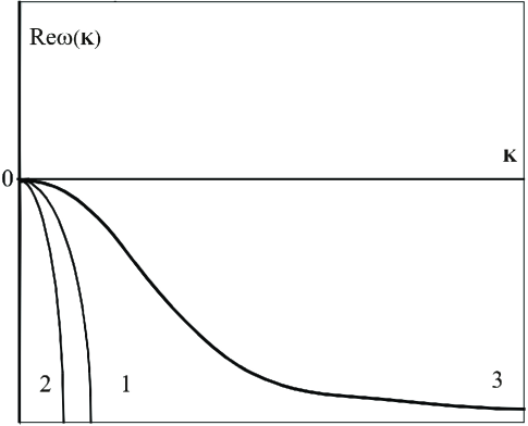
Figure 2: Attenuation rates of various modes of the post-Navier-Stokes equations as functions of the wave vector. Attenuation rate of the twice degenerated shear mode is curve 1. Attenuation rate of the two sound modes is curve 2. Attenuation rate of the diffusion mode is curve 3.

This matrix has five eigenvalues. These real parts of these eigenvalues responsible for the decay rate of the corresponding modes are shown in Fig. 2 as functions of the wave vector $k$. We see that all real parts of all the eigenvalues are non-positive for any wave vector. In other words, this means that the present system is linearly stable. For the Burnett hydrodynamics as derived from the Boltzmann or from the single relaxation time Bhatnagar-Gross-Krook model, it is well known that the decay rate of the acoustic becomes positive after some value of the wave vector [6, 20] which leads to the instability. While the method suggested here is clearly semi-phenomenological (coarse-graining time $\tau$ remains unspecified), the consistency of the expansion with the entropy requirements, and especially the latter result of the linearly stable post-Navier-Stokes correction strongly indicates that it might be more suited to establishing models of highly nonequilibrium hydrodynamics.

4.3 Diffusion in the two-component fluid

In this example we consider a mixture of the particles of two kinds. We determine microscopic equations as two independent one-particle Liouville equations. Using our general procedure, we obtain a diffusion behavior of the mixture on the macroscopic level.

Microscopic equations of motion for the particles of the first and of the second kind are:

$${\partial f_{\rm 1}\over\partial t} = -{\bf v}_{1}{\partial f_{1}\over\partial{\bf r}},$$ (61)

$${\partial f_{2}\over\partial t} = -{\bf v}_{2}{\partial f_{2}\over\partial{\bf r}}.$$ (62)

We denote all variables related to particles of the first kind with index $1$, and with the index $2$ for the second kind, $f_{1}=f_{1}({\bf r},{\bf v}_{1},t)$ and $f_{2}=f_{2}({\bf r},{\bf v}_{2},t)$ are one-particle distribution functions.

In order to describe hydrodynamics of the system, we introduce the following macroscopic variables:

$$M_{1} = \rho_{1}=m_{1}\int f_{1}d{\bf v},$$

$$M_{2} = \rho_{2}=m_{2}\int f_{2}d{\bf v},$$

$$M_{i} = (\rho_{1}+\rho_{2})u_{i}=m_{1}\int v_{1i}f_{1}d{\bf v}+m_{2}\int v_{2i}f_{1}d{\bf v},$$ (63)

$$M_{T} = {3\over 2}(n_{1}+n_{2})k_{B}T=m_{1}\int{(v_{1}-u)^{2}\over 2}f_{1}d{\bf v}+m_{2}\int{(v_{2}-u)^{2}\over 2}f_{2}d{\bf v},$$

where $\rho_{1},\,\rho_{2}$ are densities; $u_{i}$ is the i-th spatial component of the average velocity of the mixture; and $T$ is the temperature.

The quasi-equilibrium distribution functions are:

$$f_{1}=n_{1}({\bf r})\left(m_{1}\over 2\pi k_{B}T({\bf r})\right)^{3/2}\exp\left\{-{m_{1}(v_{1}-u({\bf r}))^{2}\over 2k_{B}T({\bf r})}\right\},$$ (64)

$$f_{2}=n_{2}({\bf r})\left(m_{2}\over 2\pi k_{B}T({\bf r})\right)^{3/2}\exp\left\{-{m_{2}(v_{2}-u({\bf r}))^{2}\over 2k_{B}T({\bf r})}\right\}.$$ (65)

After the convolution of the system (61)–(62) with the operators $\mu_{1}=\int m_{1}\cdot d{\bf v},$ $\mu_{2}=\int m_{2}\cdot d{\bf v},$ $\mu_{u1}=\int m_{1}v_{1}\cdot d{\bf v},$ $\mu_{u2}=\int m_{2}v_{2}\cdot d{\bf v},$ $\mu_{T1}=\int m_{1}(v_{1}-u)^{2}/2\cdot d{\bf v},$ $\mu_{T2}=\int m_{2}(v_{2}-u)^{2}/2\cdot d{\bf v}$, and after summations, we obtain the system of Euler equations for the binary mixture:

$${\partial\rho_{1}\over\partial t} = -{\partial\rho_{1}u_{i}\over\partial r_{i}},$$ (66)

$${\partial\rho_{2}\over\partial t} = -{\partial\rho_{2}u_{i}\over\partial r_{i}},$$ (67)

$${\partial\rho u_{k}\over\partial t} = -{\partial nk_{B}T\over\partial r_{k}}-{\partial\rho u_{k}u_{i}\over\partial r_{i}},$$ (68)

$${3\over 2}{\partial nk_{B}T\over\partial t} = -{3\over 2}{\partial u_{i}nk_{B}T\over\partial r_{i}}-nk_{B}T{\partial u_{i}\over\partial r_{i}}.$$ (69)

Let us now calculate the dissipative correction for the density equations. For the equation (66) we obtain:

$$R_{1} = {1\over 2}\left({\partial^{2}n_{1}k_{B}T\over\partial r^{2}}+{\partial^{2}\rho_{1}u_{i}u_{j}\over\partial r_{i}\partial r_{j}}\right)$$ (70)

$$- {1\over 2}{\partial\over\partial r_{k}}\left({M_{k}\over\rho}{\partial\over\partial r_{j}}\left({M_{j}\rho_{1}\over\rho}\right)-{M_{k}\rho_{1}\over\rho^{2}}{\partial\over\partial r_{j}}\left({M_{j}\rho_{1}\over\rho}\right)\right)$$

$$- {1\over 2}{\partial\over\partial r_{k}}\left({M_{k}\rho_{2}\over\rho^{2}}{\partial\over\partial r_{j}}\left({M_{j}\rho_{2}\over\rho}\right)\right)-{1\over 2}{\partial\over\partial r_{k}}\left\{{\rho_{1}\over\rho}{\partial nk_{B}T\over\partial r_{k}}+{\rho_{1}\over\rho}{\partial nu_{j}u_{k}\over\partial r_{j}}\right\}.$$

Substituting (63) into (70), and performing similar to the above calculations for the equation (66), we arrive at the diffusion equations for the binary mixture under a simplifying assumption $T=\textrm{const}$, ${\bf u}=0$:

$${\partial\rho_{1}\over\partial t} = {\tau k_{B}T\over 2}\left\{{\partial^{2}n_{1}\over\partial r_{k}\partial r_{k}}-{\partial\over\partial r_{k}}\left({\rho_{1}\over\rho}{\partial n\over\partial r_{k}}\right)\right\},$$ (71)

$${\partial\rho_{2}\over\partial t} = {\tau k_{B}T\over 2}\left\{{\partial^{2}n_{2}\over\partial r_{k}\partial r_{k}}-{\partial\over\partial r_{k}}\left({\rho_{2}\over\rho}{\partial n\over\partial r_{k}}\right)\right\}.$$ (72)

Diffusion coefficient $\tau k_{B}T/2m$ coincides with Einstein diffusion coefficient, where $\tau$ has meaning of the average relaxation time.

5 Hydrodynamic equation for the fluid with long-range interaction

In this section we derive equations of hydrodynamics from the nonlinear Vlasov equation. This example is also interesting from the methodological point of view. Usual methods of reduction of the description are applicable mostly to a linear microscopic dynamics [8, 7, 9]. These methods are based on a formal solution to the microscopic equation of motion presented in the exponential form. This is not directly possible for nonlinear microscopic models. Since we avoid integrating microscopic equations of motion, our approach is immediately applicable to nonlinear systems without any modifications.

Let the microscopic dynamics be given by the Vlasov equation (18). Choosing again the usual hydrodynamic fields for the macroscopic variables (42), we obtain the system of Euler equations enriched by the mean-field terms:

$${\partial n\over\partial t} = -{\partial nu_{i}\over\partial r_{i}},$$

$${\partial nu_{k}\over\partial t} = -{\partial\over\partial r_{k}}{nk_{B}T\over m}-{\partial nu_{k}u_{j}\over\partial r_{j}}+nF_{k},$$ (73)

$${\partial\varepsilon\over\partial t} = -{\partial\over\partial r_{i}}\left({5k_{B}T\over m}nu_{i}+u^{2}nu_{i}\right)+2nu_{i}F_{i},$$

where $F_{i}$ is the $i-$th spatial component of the mean-field force given by equation (19).

Following the same route as in section (4.1), we compute term by term the correction for (73). The first term in the brackets in equation (9) is proportional to:

$${\partial J^{*}\over\partial f}J^{*} = v_{i}v_{j}{\partial^{2}f_{0}\over\partial r_{i}\partial r_{j}}+v_{i}{\partial\over\partial r_{i}}\left({\partial f_{0}\over\partial v_{j}}F_{j}\right)+{\partial f_{0}\over\partial v_{i}}\Psi_{i}$$ (74)

$$+ F_{i}{\partial\over\partial v_{i}}\left(v_{j}{\partial f_{0}\over\partial r_{j}}\right)+F_{i}{\partial\over\partial v_{i}}\left({\partial f_{0}\over\partial v_{j}}F_{j}\right),$$

where $\Psi$ is given by equation(21).

In order to calculate the mean-field terms in the velocity equation, we act by the operator $\int v_{k}\cdot d{\bf v}$ on equation (74). We obtain:

$$-2\left({\partial nu_{i}\over\partial r_{i}}F_{k}+{\partial nu_{k}\over\partial r_{i}}F_{i}\right)-(nu_{i}\delta_{jk}+nu_{k}\delta_{ij}){\partial F_{j}\over\partial r_{i}}$$

$$-n\Psi_{k}+{\partial nu_{k}\over\partial r_{i}}F_{i}.$$ (75)

The second part of equation (9) is:

$$\sum_{j}{\partial\phi_{u_{i}}\over\partial M_{j}}\phi_{j}=-F_{j}M_{0}{\partial M_{i}\over\partial r_{j}}-M_{j}{\partial F_{i}\over\partial r_{j}}-F_{i}{\partial M_{j}\over\partial r_{j}}-{M_{i}\over M_{0}}{\partial F_{j}M_{0}\over\partial r_{j}}-F_{i}{\partial M_{j}\over\partial r_{j}},$$

where $M_{i}$ correspond to (42). Rewriting this expression in terms of the variables $n,{\bf u}$ and $T$, and combining the result with equation (75), we obtain:

$$R^{(1)}_{nu_{k}}=n\Psi_{k}.$$

Now let us calculate the correction to the energy equation (48) in the presence of the mean-field interaction. Action of the operator $\int v^{2}\cdot d{\bf v}$ on equation (74) gives:

$$\left(-5{\partial\over\partial r_{j}}\left({k_{B}Tn\over m}\right)-2u_{i}u_{j}{\partial n\over\partial r_{i}}-u^{2}{\partial n\over\partial r_{j}}\right)F_{j}-$$

$$\left(2nu_{i}{\partial u_{j}\over\partial r_{i}}-2nu_{i}{\partial u_{i}\over\partial r_{j}}-2nu_{j}{\partial u_{i}\over\partial r_{i}}\right)F_{j}+$$

$$\left(-5{nk_{B}T\over m}\delta_{ij}-2nu_{i}u_{j}-u^{2}n\delta_{ij}\right){\partial F_{j}\over\partial r_{i}}$$

$$-2nu_{i}\Psi_{i}+\left(3{\partial\over\partial r_{i}}\left({k_{B}Tn\over m}\right)+{\partial nu^{2}\over\partial r_{i}}\right)F_{i}+2nF_{i}F_{i}.$$

The differential term for the energy density equation gives:

$$\sum_{i}{\partial\phi_{\varepsilon}\over\partial M_{i}}\phi_{i} = -{M_{4}\over M_{0}}F_{i}{\partial M_{0}\over\partial r_{i}}-M_{4}{\partial F_{i}\over\partial r_{i}}-{2\over 3}{\partial\over\partial r_{i}}\left(F_{i}\left(M_{4}-{M_{n}M_{n}\over M_{0}}\right)\right)$$

$$- 2F_{i}M_{j}{\partial\over\partial r_{j}}\left({M_{i}\over M_{0}}\right)-2F_{j}M_{i}{\partial\over\partial r_{j}}\left({M_{i}\over M_{0}}\right)-2{M_{i}M_{j}\over M_{0}}{\partial F_{i}\over\partial r_{j}}$$

$$- F_{i}{\partial\over\partial r_{i}}\left(M_{4}-{M_{n}M_{n}\over M_{0}}\right)+{F_{i}\over M_{0}}\left(M_{4}-{M_{n}M_{n}\over M_{0}}\right){\partial M_{0}\over\partial r_{i}}$$

$$- {2M_{j}F_{j}\over M_{0}}{\partial M_{i}\over\partial r_{i}}-F_{i}{2\over 3}{\partial\over\partial r_{i}}\left(M_{4}-{M_{n}M_{n}\over M_{0}}\right)$$

$$- 2F_{i}M_{j}{\partial\over\partial r_{j}}\left(M_{i}\over M_{0}\right)-{2F_{i}M_{i}\over M_{0}}{\partial M_{j}\over\partial r_{j}}.$$

Thus, we obtain the first-order correction to the energy equation,

$$R^{(1)}_{\varepsilon}={6k_{B}T\over m}F_{i}{\partial n\over\partial r_{i}}+2F_{i}u_{i}u_{j}{\partial n\over\partial r_{j}}-2nu_{i}\Psi_{i}+2nF_{i}F_{i},$$

Finally, we arrive at the following system of hydrodynamic equations with the the mean-field interaction:

$${\partial n\over\partial t} = -{\partial nu_{i}\over\partial r_{i}},$$

$${\partial nu_{k}\over\partial t} = -{\partial\over\partial r_{k}}{nk_{B}T\over m}-{\partial nu_{k}u_{j}\over\partial r_{j}}+nF_{k}+$$ (76)

$${\tau\over 2}{\partial\over\partial r_{j}}{nk_{B}T\over m}\left({\partial u_{k}\over\partial r_{j}}+{\partial u_{j}\over\partial r_{k}}-{2\over 3}{\partial u_{n}\over\partial r_{n}}\delta_{kj}\right)-{\tau n\over 2}\Psi_{k},$$

$${\partial\varepsilon\over\partial t} =- {\partial\over\partial r_{i}}\left({5k_{B}T\over m}nu_{i}+u^{2}nu_{i}\right)+2nu_{i}F_{i}+$$

$$\tau{5\over 2}{\partial\over\partial r_{i}}\left({nk_{B}^{2}T\over m^{2}}{\partial T\over\partial r_{i}}\right)+\tau{3k_{B}T\over m}F_{i}{\partial n\over\partial r_{i}}+\tau F_{i}u_{i}u_{j}{\partial n\over\partial r_{j}}-$$

$$\tau nu_{i}\Psi_{i}+\tau nF_{i}F_{i},$$

Equations (76) are the general form of the hydrodynamic equations of a simple fluid with the mean-field interaction. Examples of the system for which this result may be relevant can be found in studies of electron transport in the various media [19], as well as in description of non-Newtonian fluids [22]. For each particular case the interaction potential $\Phi(|{\bf r}-{\bf r}^{\prime}|)$ has its specific form, and leads to the corresponding hydrodynamics of the system.

6 Conclusion

In this paper the formalization of Ehrenfest’s approach to irreversible dynamics is given in details. This method allows one to derive macroscopic equations of motion on the basis of the microscopic dynamics and the very transparent coarse-graining procedure. The method is applicable to both reversible as well as to the irreversible microscopic dynamics, independently of whether it is linear or not. We have presented a set of examples demonstrating how this method is applied to various situations.

The most interesting continuation of this approach is, of course, how to specify in a sensible and practical way the coarse-graining time $\tau$ in order to make the modelling parameter-free. This requires is a subject of our current studies (see [23, 24, 25]).

Finally, whereas we have focused on the application of our formalism to the entropy-conserving microscopic dynamics, it should be mentioned that it is applicable also to constructing slow invariant manifolds of dissipative systems. In particular, when applied to the Boltzmann equation, the result is equivalent at $\tau\to\infty$ to the exact Chapman-Enskog solution [23].

Figure 1: Coarse-graining scheme. $f$ is the space of microscopic variables, $M$ is the space of the macroscopic variables, $f^{*}$ is the quasi-equilibrium manifold, $\mu$ is the mapping from the microscopic to the macroscopic space.

References

• [1] L. Boltzmann, Lectures on the Theory of Gases, University of California Press, (1964)
• [2] P. Ehrenfest and T.  Ehrenfest, Encyklopädie der Mathematischen Wissenschaften, Bd. IV 2, II, H. 6 (1911) [Reprinted in: P. Ehrenfest, Collected Scientific Papers, North-Holland, Amsterdam, (1959)
• [3] Studies in Statistical Mechanics, edited by E. W. Montroll and J. L. Lebowitz, North-Holland, (1981), Vol. 9.
• [4] J. L. del Ro-Correa and L. S. Garsa-Coln, Phys. Rev. E 48, 819 (1993).
• [5] A. N. Gorban, I. V. Karlin, H. C. Öttinger, and L. L. Tatarinova, Phys. Rev. E 63, 066124 (2001).
• [6] A. V. Bobylev, Dokl. Akad. Nauk (SSSR) 262, 71 (1982), [Sov. Phys. Dokl. 27, 29 (1982)].
• [7] D. Zubarev, V. Morosov, and G. Röpke, Statistical Mechanics of Nonequilibrium Processes, Akademie Verlag, Berlin, (1996), Vol. 1.
• [8] B. Robertson, Phys. Rev. 44, 151 (1966).
• [9] H. Grabert, Projection Operator Techniques in Nonequilibrium Statistical mechanics, Springer, Berlin, (1982).
• [10] E. T. Jaynes, Phys. Rev. 106, 620 (1957); 108, 171 (1957).
• [11] A. N. Gorban, Equilibrium Encircling, Nauka, Novosibirsk, (1984).
• [12] R. M. Lewis, J. Math. Phys. 8, 1448 (1967).
• [13] O. Pashko and Y. Oono, Int. J. Mod. Phys. B 14, 555 (2000).
• [14] E. M. Lifschitz and L. P. Pitaevsky Physical Kinetic, Pergamon Press, Oxford, (1980).
• [15] P.Résibois and M. De Leener, Classical Kinetic Theory of Fluids, Wiley, NY, (1977).
• [16] S. Chapman and T.  G.  Cowling. The Mathematical Theory of Non-uniform Gases, Cambridge University Press, Cambridge, (1970).
• [17] A. N. Gorban, I. V. Karlin, P. Ilg, and H. C. Öttinger, J. Non-Newtonian Fluid Mech. 96, 203 (2001).
• [18] H. C. Öttinger, Stochastic Processes in Polymeric Fluids. Tools and Examples for Developing Simulation Algorithms (Springer, Berlin etc, 1996).
• [19] R. Balescu. Transport Processes in Plasmas, Classical Transport Theory, North-Holland, Amsterdam, (1988), Vol. 1.
• [20] I. V. Karlin and A. N. Gorban, Ann. Phys. (Leipzig) 11, 783 (2002).
• [21] P. L. Bhatnagar, E. P. Gross, and M. Krook, Phys. Rev. 94, 511 (1954).
• [22] A. N. Gorban, I. V. Karlin, and L. L. Tatarinova (unpublished).
• [23] A. N. Gorban and I. V. Karlin, Phys. Rev. E 65, 026116 (2002).
• [24] A. N. Gorban and I. V. Karlin, Rev. Mex. Fís. 48 S1, 238 (2002).
• [25] A. N. Gorban and I. V. Karlin, in: Developments in Mathematical and Experimental Physics, Volume C: Hydrodynamics and Dynamical Systems, Eds. A. Macias, F. Uribe and E. Diaz (Kluwer, New York, 2003).
Refer to caption