The GPE and higher order theories in one-dimensional Bose gases

Abstract

We investigate the properties of the one-dimensional Bose gas at zero temperature, for which exact results exist for some model systems. We treat the interactions between particles in the gas with an approximate form of the many-body T-matrix, and find a form of Gross-Pitaevskii equation valid in 1D. The results presented agree with the exact models in both the weakly and strongly interacting limits, and interpolate smoothly between them. We also investigate the use of mean-field treatments of trapped BECs to describe the 1D system in the strongly interacting limit. We find that the use of the many-body T-matrix to describe interactions leads to qualitative agreement with the exact models for some physical quantities. We indicate how the standard mean-field treatments need to be modified to extend and improve the agreement.

I Introduction

Recent advances in experimental techniques Görlitz et al. (2001); Schreck et al. (2001) have stimulated interest in the topic of ultra-cold dilute Bose gases in one dimension. The one-dimensional (1D) case leads to some interesting physics which does not occur in higher dimensions, and is also of theoretical importance due to the existence of exactly soluble models Girardeau (1960); Lieb and Liniger (1963); Lieb (1963). In this paper we investigate the 1D Bose gas in the limit of zero temperature. We extend our earlier work Lee et al. (2002) on the interactions in two dimensions to the 1D case, and obtain a 1D form of Gross-Pitaevskii equation (GPE). We also apply standard methods of mean-field theory developed to describe three-dimensional Bose-Einstein condensates (BECs) to the 1D trapped case. In both cases we compare the results obtained from these methods to the exact solutions.

It is well known that a true BEC cannot occur at any finite temperature in an interacting homogeneous Bose gas in 1D Hohenberg (1967), due to long wavelength fluctuations; nor can it occur in the limit of zero temperature Pitaevskii and Stringari (1991), due to quantum fluctuations. However, the presence of a trapping potential changes the density of states at low energies, and in the weakly-interacting limit a BEC may be formed Ketterle and van Druten (1996). In a recent paper, Petrov et al. discussed three different regimes of quantum degeneracy which can occur in a confined 1D interacting system Petrov et al. (2000): BEC, quasi-condensate, and Tonks-Girardeau gas. In the weakly interacting limit a BEC exists, but as the interactions become stronger the mean-field energy becomes important. When this energy becomes of the order of the energy level spacing of the trap, fluctuations again become significant. In this regime, the system forms a quasi-condensate, with local phase coherence, rather than the global coherence associated with a true BEC. In this regime the gas is similar to the homogeneous case, in which it was shown that at $T=0$ the phase coherence has only a power-law decay, rather than the exponential decay occurring at higher temperatures Schwartz (1977). Finally, in the limit of very strong interactions, the particles become impenetrable and the system is known as a Tonks-Girardeau gas Tonks (1936); Girardeau (1960). This limit is exactly soluble, due to a mapping relationship between the wave function for the bosons and that of a non-interacting fermion gas Girardeau (1960).

In the following section we briefly outline the relevant exact results for a 1D gas. Section III then presents a form of the GPE in which we use an approximate many-body T-matrix to describe the interactions in a 1D gas. The GPE gives the correct results in both the weakly-interacting and Tonks-Girardeau limits, and interpolates smoothly between these regimes. We confirm that the non-linear dependence in the GPE changes from cubic in the weakly-interacting regime to quintic in the strongly-interacting regime, and that this arises due to the many-body effects on the scattering of particles. In Sec. IV, we then discuss several standard mean-field theories and present the results of these for the trapped 1D gas. In the weakly interacting limit these theories should be valid since a true BEC exists in this regime. Our aim is to push several different theories into the strongly-interacting limit with the dual objectives of describing the 1D system and investigating the strengths and weaknesses of these theories.

II Exact results in 1D

The 1D homogeneous system of $N$ bosons which interact via a delta-function potential of the form

$$V(x_{1}-x_{2})=V_{0}\delta(x_{1}-x_{2}),$$ (1)

is exactly integrable. In the limit $V_{0}\rightarrow\infty$ the particles are impenetrable (the Tonks-Girardeau gas), and exact results can be obtained even in spatially inhomogeneous systems. The exact solutions are found by applying the appropriate boundary conditions to the wave function describing the system.

In the impenetrable limit the wave function must necessarily vanish wherever two particles meet (i.e. wherever $x_{i}=x_{j}$). Girardeau showed in Girardeau (1960) that the exact $N$-boson ground state wave function subject to such a boundary condition is equal to $|\psi_{F}(x_{1},...,x_{N})|$, where $\psi_{F}(x_{1},...,x_{N})$ is the wave function of $N$ non-interacting spinless fermions governed by the single-particle Hamiltonian $\hat{H}_{\rm sp}$ (including terms from any external potential). Since the wave functions of such fermions must be antisymmetric with respect to co-ordinate exchanges, their wave functions automatically vanish whenever $x_{i}=x_{j}$, and so the Tonks-Girardeau gas boundary condition is implicitly obeyed by such a gas.

A number of bulk properties of a 1D Tonks-Girardeau gas may be calculated quite trivially as a result of this Fermi-Bose mapping theorem Girardeau (1960); Girardeau et al. (2001). For example, the ground state energy of a Tonks-Girardeau gas is simply found from a summation of the energies of the first $N$ non-interacting single-particle states (i.e. those that would be occupied by $N$ ideal fermions in the ground state configuration). Thus, for a homogeneous gas Girardeau (1960)

$${E_{0}\over N}={\hbar^{2}\over m}{\pi^{2}\over 6}n^{2},$$ (2)

where $n$ is the density. The chemical potential is then easily calculated as

$$\mu={\partial E_{0}\over\partial N}={\hbar^{2}\over m}{\pi^{2}\over 2}n^{2}.$$ (3)

Similarly, the chemical potential for a Tonks-Girardeau gas in a harmonic potential of frequency $\omega$ is

$$\mu=\hbar\omega(N+1/2).$$ (4)

The system of $N$ bosons interacting with an arbitrary value of $V_{0}$ was solved in 1963 by Lieb and Liniger Lieb and Liniger (1963); Lieb (1963) for a homogeneous gas. The Tonks-Girardeau gas results are recovered in the limit $V_{0}\rightarrow\infty$. The ground-state energy of the Lieb-Liniger gas is given (at $T=0$) by

$${E_{0}\over N}={\hbar^{2}\over 2m}n^{2}e(\gamma),$$ (5)

where $e(\gamma)$ is a solution to the Lieb-Liniger system of equations, and is a function of the dimensionless quantity $\gamma=V_{0}m/\hbar^{2}n$ which was found to be the important parameter in the system. The function $e(\gamma)$ has the following asymptotic behaviour

$$e(\gamma)\approx\left\{\begin{array}[]{ll}\gamma&\mbox{ for }\gamma\rightarrow 0,\\ {\pi^{2}\over 3}\left({\gamma\over\gamma+2}\right)&\mbox{ for }\gamma\rightarrow\infty,\end{array}\right.$$ (6)

and the energy per particle agrees with Eq. (2) in the impenetrable limit. The chemical potential is given by the equation

$$\mu={\hbar^{2}\over 2m}n^{2}\left[3e(\gamma)-\gamma{de(\gamma)\over d\gamma}\right].$$ (7)

In the $\gamma\rightarrow 0$ weakly-interacting limit, the exact results were found to be in agreement with the predictions of standard Bogoliubov theory. The Bogoliubov predictions begin to fail as $\gamma$ is increased and for $\gamma\gtrsim 2$ the results do not agree well with the exact theory Lieb and Liniger (1963). Interestingly, for fixed $V_{0}$ the $\gamma\rightarrow 0$ limit corresponds to the high-density limit, whilst a high value of $\gamma$ implies a small density. This is then the reverse of the 3D case where Bogoliubov theory is valid in the low density limit. In a subsequent section we will show to what extent higher-order modifications to Bogoliubov theory can improve the agreement for higher $\gamma$.

For a system where we keep the density constant, and increase the interaction strength $V_{0}$ from the non-interacting limit to the impenetrable limit (i.e. increasing $\gamma$), we expect the chemical potential to vary in the following manner. In the low-$V_{0}$ limit the chemical potential increases linearly with $V_{0}$, but as $V_{0}$ is increased further $\mu$ starts to saturate, and in the high-$V_{0}$ limit it becomes independent of $V_{0}$, in agreement with Eq. (3). In the following section we introduce a modified GPE which follows this behaviour.

III The GPE in 1D

We consider the model system of a gas of one-dimensional point particles interacting with an arbitrary strength $V_{0}$, corresponding to the Lieb-Liniger gas. We emphasize here that we are interested in the limit in which the interparticle interactions in the system are genuinely one-dimensional, because it is only in this limit that we can compare to the exact results mentioned earlier.

We can write a one-dimensional Gross-Pitaevskii equation for a system of $N$ particles by a straightforward generalisation of the usual 3D equation, giving

$$\mu\psi(x)=\left[-{\hbar^{2}\over 2m}{d^{2}\over dx^{2}}+V_{\rm trap}(x)+g_{\rm 1D}N|\psi(x)|^{2}\right]\psi(x),$$ (8)

where $\psi(x)$ is the condensate wave function, and $V_{\rm trap}(x)$ represents the trapping potential. The coupling parameter $g_{\rm 1D}$ describes the interactions between particles, and we discuss the nature of this quantity in the following section before presenting the results predicted by the GPE.

III.1 Interactions and the GPE

The GPE can easily be derived by functional differentiation of the Hamiltonian for a gas with a general interparticle interaction $V(x)$. The coupling parameter is then given by the matrix element $\langle 0|V(x)|0\rangle$, where the particles in both the incoming and outgoing states have zero relative momentum (see, for example, Morgan (2000)). However, a representation in terms of matrix elements of the bare interparticle potential is undesirable, since for a realistic potential they are often very large and frequently the exact potential itself is unknown. In order to avoid this it is common for 3D problems to use the two-body T-matrix $T_{\rm 2B}$ in place of the interparticle potential. This T-matrix describes the scattering of two particles in a vacuum, and it is possible to rewrite the interaction term in the Hamiltonian in terms of $T_{\rm 2B}$ Morgan (2000). Carrying out the functional differentiation again leads to a GPE of the above form, where the coupling parameter is now $g=\langle 0|T_{\rm 2B}(E=0)|0\rangle$. Here $E$ is the energy of the interacting particles, and for two condensate particles this is zero. In three dimensions this leads to the familiar result $g_{\rm 3D}=4\pi\hbar^{2}a/m$, where $a$ is the s-wave scattering length. However, in 1D (and 2D) the two-body T-matrix vanishes in the zero energy and momentum limit, and has significant imaginary terms at a finite real energy (see, for example, Morgan et al. (2002)).

In earlier papers Lee et al. (2002); Lee and Morgan (2002), we have argued that the many-body effects of the surrounding atoms on particle interactions, while being a small perturbation in 3D, are crucial in lower dimensions. The many-body effects can be incorporated into a many-body T-matrix $T_{\rm MB}$ Stoof et al. (1996); Bijlsma and Stoof (1997); Proukakis et al. (1998); Morgan (2000), and the coupling parameter in the GPE becomes

$$g_{\rm 1D}=\langle 0|T_{\rm MB}(E=0)|0\rangle.$$ (9)

Unfortunately, the many-body T-matrix is very difficult to solve exactly. However, in Lee et al. (2002) we presented an approximate solution, valid in the zero temperature limit, in which the many-body T-matrix was approximated by the two-body T-matrix evaluated at a shifted effective interaction energy (off the energy shell). The GPE in 1D is therefore given by Eq. (8) with the coupling parameter

$$g_{\rm 1D}=\langle 0|T_{\rm MB}(E=0)|0\rangle\approx\langle 0|T_{\rm 2B}(E^{*})|0\rangle,$$ (10)

where $E^{*}$ is the shifted interaction energy, and was found in Lee et al. (2002) to be negative. As an illustration of the utility and accuracy of this approximation, we discuss its application to the 3D case in the appendix.

III.2 The hard-core limit

We will look first at the GPE in the impenetrable, $V_{0}\rightarrow\infty$, limit in which the system is a Tonks-Girardeau gas. The off-shell two-body T-matrix for such a 1D gas, calculated in Morgan et al. (2002), is

$$\langle 0|T_{\rm 2B}^{\rm Tonks}(E)|0\rangle=$$ (13)

$$\left\{\begin{array}[]{ll}-\frac{2\hbar^{2}}{ma}\left(i\sqrt{mE\over\hbar^{2}}a+{mE\over\hbar^{2}}a^{2}\right)&\mbox{for }E>0,\\ -\frac{2\hbar^{2}}{ma}\left(\sqrt{m|E|\over\hbar^{2}}a-{mE\over\hbar^{2}}a^{2}\right)&\mbox{for }E<0,\end{array}\right.,$$

where $a$ is the size of the impenetrable particle, and for the delta-function gas we take the limit that $a\rightarrow 0$. Combined with Eq. (10) this gives a coupling parameter of the form Lee et al. (2002)

$$g_{\rm Tonks}(\mu)=\sqrt{4C\hbar^{2}\mu/m}$$ (14)

to leading order for a homogeneous system. Here we have taken $E^{*}=-C\mu$ and assumed that $C>0$ Lee et al. (2002), (note that if this is not the case then the coupling parameter is imaginary to leading order). Using the homogeneous solution to the GPE $\mu=g_{\rm Tonks}n$ we can rewrite the coupling parameter in terms of the density $n$ as

$$g_{\rm Tonks}(n)={4C\hbar^{2}\over m}n.$$ (15)

Combining this with $\mu=g_{\rm Tonks}n$ gives $\mu\propto n^{2}$, and a comparison with the exact result found by Girardeau and given in Eq. (3), shows that we have obtained the correct functional dependence of $\mu$ on $n$. This stems from the dependence of the coupling parameter on $\sqrt{\mu}$ in Eq. (14). This is further verification of our approximation for the many-body T-matrix in terms of the off-shell two-body T-matrix. A comparison with the Girardeau result also shows that $C=\pi^{2}/8$.

To apply this result to a trapped system, we use a local density approximation, assuming that the scattering between two particles occurs on a length scale much shorter than the variation in the potential. First we solve the homogeneous expression $\mu=g_{\rm Tonks}(\mu)n$ to obtain an expression for the chemical potential in terms of the density $n$. Applying the local density approximation then requires $\mu(n(x))=g_{\rm Tonks}(x)n(x)$ to hold for all $x$, and we obtain a spatially-dependent coupling parameter

$$g_{\rm Tonks}(x)={\pi^{2}\hbar^{2}N\over 2m}|\psi(x)|^{2},$$ (16)

where we have used $n(x)=N|\psi(x)|^{2}$.

We can now write the GPE for a 1D trapped condensate as

$$\mu\psi(x)=\left[-{\hbar^{2}\over 2m}{d^{2}\over dx^{2}}+V_{\rm trap}(x)+{\pi^{2}\hbar^{2}N^{2}\over 2m}|\psi(x)|^{4}\right]\psi(x).$$ (17)

This GPE differs significantly from the 3D version by virtue of the fact that the nonlinear term is now proportional to $|\psi|^{4}\psi$ instead of $|\psi|^{2}\psi$. In the Thomas-Fermi limit we can neglect the kinetic energy term and the solution for the wave function can easily be shown to be

$$|\psi(x)|={\left(\mu-V_{\rm trap}(x)\right)^{1/4}\over(\hbar^{2}\pi^{2}N^{2}/2m)^{1/4}}\theta\left(\mu-V_{\rm trap}(x)\right)$$ (18)

This differs substantially from the 3D and 2D cases, where the Thomas-Fermi wave function is instead proportional to $(\mu-V_{\rm trap}(x))^{1/2}$, due to the different form of the non-linearity.

The Tonks-Girardeau GPE and the results presented in this section are in exact agreement with the earlier work of Kolomeisky et al. Kolomeisky et al. (2000), who obtained the same form of coupling parameter from a renormalisation group approach Kolomeisky and Straley (1992).

In Fig. 1a we present a comparison of the density $N|\psi|^{2}$ obtained from the solution of the GPE of Eq. (17) with the exact result from the Bose-Fermi mapping theorem calculated by a summation of the first $N$ single-particle states of the trap. It can be seen that the GPE solution is in very good agreement with the exact result, and differs only in the absence of the oscillations seen in the exact result. These oscillations rapidly average out as the number of atoms is increased, and for a moderately large number the difference between the GPE results and the exact results will be negligible.

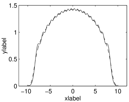
Figure 1: (a) Comparison of ground state density for Tonks gas (solid) and density calculated from Eq. (17) with $|\psi|^{4}\psi$ non-linearity (dashed), both with $\mu=20\hbar\omega$ and $N=20$.

III.3 The delta-function potential

We now turn to a discussion of the Lieb-Liniger gas. We are interested here in describing the gas from the non-interacting limit right through to the Tonks-Girardeau limit by means of an appropriate GPE.

The same argument which we used in deriving the Tonks-Girardeau GPE can again be used, namely that the coupling parameter should be the many-body T-matrix. Again we approximate this by a two-body T-matrix evaluated off the energy shell at an energy of $-C\mu$, where we use the value of $C=\pi^{2}/8$ obtained above.

The two-body T-matrix for a delta-function potential is given by Morgan et al. (2002)

$$\langle 0|T_{\rm 2B}^{\rm LL}(E)|0\rangle=\frac{V_{0}}{1+iV_{0}\displaystyle{\left(\frac{m}{2\hbar^{2}}\right)\sqrt{\frac{\hbar^{2}}{mE}}}}.$$ (19)

Note that for $V_{0}\rightarrow\infty$, this reduces to the Tonks limit of Eq. (13). It follows that our approximation for the many-body T-matrix in a homogeneous 1D system is

$$g_{\rm LL}(\mu)=\frac{V_{0}}{1+V_{0}\displaystyle{\sqrt{\frac{2m}{\hbar^{2}}\frac{1}{\pi^{2}\mu}}}}.$$ (20)

This energy-dependent form of the coupling parameter can be transformed to a density-dependent expression by means of the local density approximation, as outlined above. This leads to the expression

$$g_{\rm LL}(x)=$$

$${1\over n(x)}\left(\sqrt{{m\over 2\pi^{2}\hbar^{2}}V_{0}^{2}+V_{0}n(x)}-\sqrt{{m\over 2\pi^{2}\hbar^{2}}}V_{0}\right)^{2},$$

which describes an inhomogeneous system. Note that this expression gives the correct results for the homogeneous gas in the extreme limits $V_{0}\rightarrow 0$ and $V_{0}\rightarrow\infty$, giving $\mu=nV_{0}$ and Eq. (3) respectively.

Thus we can now use the above density-dependent expression for the coupling parameter in Eq. (8) to obtain a GPE for a trapped 1D gas for any arbitrary $V_{0}$.

We use the GPE here to describe the system over the full range of $V_{0}$, despite the fact that, as mentioned earlier, a true BEC only exists in a trap in the weakly-interacting limit Petrov et al. (2000). Once the interactions cause sufficient perturbation to the density of states that their discrete nature is smeared out then no condensate will form in 1D, and in the very high-$V_{0}$ (Tonks) limit it is known that there is no condensate. We can still use the GPE in the high-$V_{0}$ regime however, as our previous results have shown, provided that we now reinterpret the “wave function” as simply the square root of the density $\psi(x)=\sqrt{n(x)}$, rather than the coherent part of the field operator.

III.3.1 The Homogeneous Case

In the homogeneous case we can compare the results of the GPE with the interaction strength given by Eq. (III.3) to the exact results for a Lieb-Liniger gas. In Fig. 2 we compare the chemical potentials resulting from the GPE with the exact result of Eq. (3). The results from the GPE show the correct behaviour in the two extreme limits of $\gamma$, and the overall agreement is quite good. However, the chemical potential of the exact results can be seen to rise more steeply in the intermediate region. We note that the results have been obtained using a value of $C$ which strictly applies only in the large $\gamma$ limit. A larger value of $C$ gives a curve which agrees very well with the exact results in the weakly-interacting regime, but predicts the wrong value in the large $\gamma$ limit. It seems possible therefore that the value of $C$ should actually be dependent on $\gamma$, but a detailed investigation of this is outside the scope of this paper.

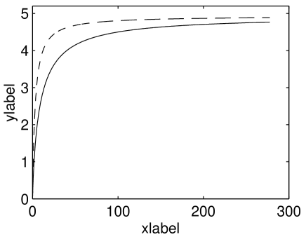
Figure 2: The chemical potential as a function of the parameter $\gamma$ for the homogeneous Lieb-Liniger gas. The dashed line shows the exact solution from the Lieb-Liniger equations Lieb and Liniger (1963), while the solid line shows the prediction of the GPE with the coupling parameter given in Eq. (20). Note that in the extremely high $\gamma$ limit (not shown) both lines have the same asymptotic value.

III.3.2 The Trapped Case

We now turn to the case of a trapped gas, where we will parameterise our results both by the interaction strength $V_{0}$ and by the dimensionless parameter $\gamma_{\rm trap}=V_{0}m/\hbar^{2}\tilde{n}_{0}$ where $\tilde{n}_{0}$ is the peak density of the system (analogous to the parameter used by Lieb and Liniger).

We expect that in the low-$V_{0}$ (small $\gamma_{\rm trap}$) limit the chemical potential will vary as

$$\mu\propto V_{0}^{2/3},$$ (22)

which is the Thomas-Fermi result obtained from the GPE with a cubic non-linearity (this is not quite the correct prediction in the extremely low-$V_{0}$ limit where the Thomas-Fermi approximation is invalid, but it should describe the majority of the low-$V_{0}$ regime adequately) . In the opposite high-$V_{0}$ limit, the Bose-Fermi mapping theorem for the trapped Tonks-Girardeau gas led to Eq. (4) which is completely independent of $V_{0}$. Note that our derivation of the GPE in Eq. (8) neglected terms of order $1/N_{0}$ since it was derived in the high-$N_{0}$ limit. For this reason we should expect only to reach an asymptotic chemical potential of $\mu=N_{0}\hbar\omega$, which is approximately equal to Eq. (4) in this limit.

Figure 3 shows sample solutions to the GPE for a range of $V_{0}$ for $N_{0}=15$. In the weakly-interacting limit the wave function can clearly be seen to be a gaussian, as expected. However as the interactions are increased the wave function broadens until in the high-$V_{0}$ limit we have the shape discussed earlier in the hard-core case. Figure 4 shows the increase in the chemical potential over the same range. As expected from the exact results for the hard-core gas, in the high-$V_{0}$ limit the chemical potential becomes almost independent of the interaction strength. For the data shown the chemical potential does not appear to quite reach the limit $\mu=N_{0}\hbar\omega$ expected from the exact results. However, in a calculation with the extreme value of $V_{0}=10^{4}\hbar\omega\ell_{\rm trap}$ we obtained the result $\mu=15.00\hbar\omega$ as expected. This agrees with the behaviour found by Lieb and Liniger in the homogeneous case, who found that the results reached the asymptotic limit very slowly (e.g. for $\gamma\approx 4$ the chemical potential had only reached $\sim 0.9$ of its asymptotic value Lieb and Liniger (1963)).

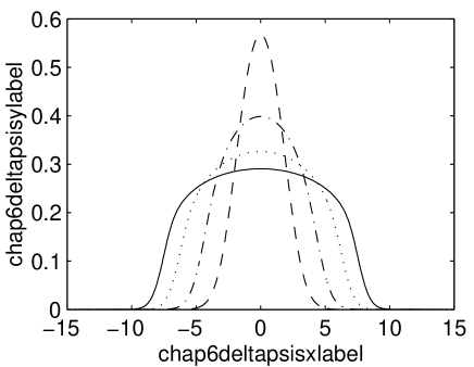
Figure 3: Solutions to the GPE for a 1D gas of $15$ atoms interacting via a delta-function potential. The dashed curve corresponds to the weakly-interacting limit with $V_{0}=0.2\hbar\omega\ell_{\rm trap}$. The dot-dash and dotted curves correspond to $V_{0}=3\hbar\omega\ell_{\rm trap}$ and $V_{0}=17\hbar\omega\ell_{\rm trap}$ respectively, while the solid line is close to the impenetrable gas limit with $V_{0}=250\hbar\omega\ell_{\rm trap}$. These values correspond to $\gamma_{\rm trap}=0.02$, $0.63$, $5.3$ and $99$ respectively.

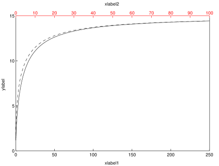
Figure 4: The chemical potential for a gas of $15$ atoms interacting via a delta-function potential as a function of the potential strength (solid line) and the parameter $\gamma_{\rm trap}$ (dashed line and upper axis).

We have therefore presented a form of the GPE in which the coupling parameter is an approximate many-body T-matrix given by the off-shell two-body T-matrix. We have shown that it agrees with the exact results for the Lieb-Liniger gas in the weakly-interacting and strongly-interacting limits, and it provides an interpolation between these limits in the intermediate regime. A drawback of using this GPE is that we lose any information about the coherences involved in the system, since we reinterpret the equation simply in terms of the density in the high-$V_{0}$ limit. The concept of using the many-body T-matrix in the GPE stemmed initially from higher order theories in which it appears naturally via the anomalous average (defined below). We therefore turn, in section IV, to an exploration of these theories in 1D and see how the changes in the interaction strength arise naturally.

III.3.3 Quasi-1D gases

Although we have been dealing with the case of a model delta-function potential gas, the results can to some extent be mapped onto those for a quasi-1D system. In practice, a 1D system could be created by squeezing a 3D trapped gas condensate in two dimensions. As the confinement is increased, the system progresses from being 3D to being 1D, via an intermediate regime we call quasi-1D for the purposes of this paper. In this intermediate regime, the dynamics of the system as a whole are frozen out in two dimensions, but the scattering between particles is not yet genuinely one-dimensional.

In the 3D regime the system is described by a GPE with a $|\psi|^{2}\psi$ nonlinearity, as for the low $V_{0}$ Lieb-Liniger gas. However, in the strict 1D limit the atoms will be unable to scatter past one another, and will form a Tonks-Girardeau gas. In this limit the appropriate GPE will be that of Eq. (17). The progression from a 3D gas to a 1D gas therefore mirrors in many respects the progression which occurs if the potential strength $V_{0}$ is increased for the Lieb-Liniger gas. The 3D to 1D progression has been investigated in more detail in references Olshanii (1998); Dunjko et al. (2001); Bergeman et al. (2002).

IV Higher order theories in 1D

In the previous section we used the GPE in conjunction with an approximate many-body T-matrix in order to describe the Lieb-Liniger gas. In this section we examine the suitability of higher-order theories to describe this gas. Ideally we would like a theory which makes the transition between the weakly interacting and strongly-interacting regimes smoothly, and which accurately describes the coherence of the system as well as the densities. There are several higher order theories which are used to good effect to describe 3D condensates, and in this section we will apply some of these to the 1D trapped gas case.

Since we can always choose a value of $V_{0}$ to be sufficiently weak that a condensate does exist in a trapped zero-temperature 1D gas, there will always be a regime in which the 3D theories can be applied. As we increase $V_{0}$ the condensate is replaced by a quasicondensate with only short range phase coherence, and this will lead to problems in the higher order theories. However, we have described in the previous section the behaviour that we expect in the high-$V_{0}$ limit. It is therefore of interest to apply the higher order theories to see how and why they fail in this limit, and to gain insight into any improvements needed to describe the 1D gas adequately.

As we have seen, the many-body effects on interactions are fundamental in understanding the behaviour of low dimensional BECs. We must therefore use a theory in which these effects are accounted for accurately. Such a theory is provided by the gapless-Hartree-Fock-Bogoliubov (GHFB) theory Proukakis et al. (1998); Hutchinson et al. (2000). In this theory, the condensate wave function $\psi_{0}(x)$ is described by the generalised GPE in 1D

$$\mu\psi_{0}(x) = -{\hbar^{2}\over 2m}{d^{2}\over dx^{2}}\psi_{0}({\bf r})+V_{\rm trap}(x)\psi_{0}(x)$$ (23)

$$\mbox{}+N_{0}U_{\rm con}(x)|\psi_{0}(x)|^{2}\psi_{0}(x)$$

$$\mbox{}+2U_{\rm ex}(x)\rho(x)\psi_{0}(x).$$

Here $\rho(x)$ is the non-condensate density and it is defined, along with the associated anomalous average $\kappa$ [needed in Eq. (29)], by

$$\rho(x) = \sum_{i\neq 0}\left(|u_{i}(x)|^{2}+|v_{i}(x)|^{2}\right)n_{i}+|v_{i}(x)|^{2},$$ (24)

$$\kappa(x) = \sum_{i\neq 0}u_{i}(x)v_{i}^{*}(x)\left(2n_{i}+1\right).$$ (25)

The Bogoliubov functions $u_{i}(x)$ and $v_{i}(x)$ are the solutions of

$$\begin{array}[]{lcr}{\cal L}(x)u_{i}(x)+{\cal M}(x)v_{i}(x)&=&\varepsilon_{i}u_{i}(x),\\[5.69054pt] {\cal L}(x)v_{i}(x)+{\cal M}^{*}(x)u_{i}(x)&=&-\varepsilon_{i}v_{i}(x),\end{array}$$ (26)

solved in a basis orthogonal to $\psi_{0}(x)$, and with

$${\cal L}(x) = \hat{H}_{\rm sp}-\mu+2N_{0}U_{\rm con}(x)|\psi_{0}(x)|^{2}$$ (27)

$$\mbox{}+2U_{\rm ex}(x)\rho(x),$$

$${\cal M}(x) = N_{0}U_{\rm con}(x)\psi_{0}^{2}(x).$$ (28)

The quasiparticle population factors $n_{i}$ are given by the Bose-Einstein distribution function, and for the zero temperature case we are concerned with here these factors vanish.

This theory distinguishes between the interactions which occur between two condensate atoms (governed by $U_{\rm con}(x)$), and those which occur between a condensate atom and a non-condensate atom (governed by $U_{\rm ex}$). The various higher order theories which we will explore in this section can now be summarised thus:

BdG

By setting $U_{\rm ex}=0$ (i.e. neglecting interactions between the condensate and the non-condensate), and using $U_{\rm con}(x)=V_{0}$, we obtain the familiar GPE and Bogoliubov-de Gennes equations.

HFB-Popov

The HFB-Popov theory corresponds to the choice $U_{\rm con}({\bf r})=V_{0}$ and $U_{\rm ex}({\bf r})=V_{0}$. Thus both condensate-condensate interactions and condensate-non-condensate interactions are included, although many-body effects on the interaction strength are not.

GHFB1

The first version of the GHFB theory is given by setting $U_{\rm con}({\bf r})=T_{\rm MB}({\bf r})$ [defined in Eq. (29)] and $U_{\rm ex}({\bf r})=V_{0}$. This version of GHFB therefore improves upon the description of the BdG or HFB-Popov descriptions by including many-body effects on the scattering of two condensate atoms.

GHFB2

From the above arguments it is clear that another GHFB theory may be proposed. This consists of setting $U_{\rm con}({\bf r})=T_{\rm MB}({\bf r})$ and $U_{\rm ex}({\bf r})=T_{\rm MB}({\bf r})$, which upgrades the description of both condensate-condensate interactions and condensate-non-condensate interactions to the many-body T-matrix.

In the GHFB theories, the many-body T-matrix is given by Proukakis et al. (1998); Morgan (2000)

$$T_{\rm MB}(x)=V_{0}\left(1+{\kappa(x)\over N_{0}\psi_{0}^{2}(x)}\right),$$ (29)

and so we can see that the inclusion of the anomalous average leads to the inclusion of the many-body T-matrix in the theories.

Note that we may use the bare potential $V_{0}$ throughout these equations, since we consider the model Lieb-Liniger system in which the interaction potential truly is a delta function. Furthermore, in 1D there is an absence of the ultra-violet divergences which occur in other dimensions when a contact potential is used. Since the above equations are always solved self-consistently, we still generate the many-body T-matrix (where used) to all orders from the bare potential Proukakis et al. (1998).

IV.1 Condensate and quasi-condensate properties

We start our simulations in the weakly-interacting limit with a small value of $V_{0}$. In this limit Lieb and Liniger Lieb and Liniger (1963) found that the Bogoliubov theory gave a good description of the homogeneous system, and so we expect our model should also be valid. We solve the above equations self-consistently to obtain the wave function, chemical potential, many-body T-matrix, $\rho(x)$, and $\kappa(x)$. We then ramp up the value of $V_{0}$, using the results from the previous iteration as our starting point. By this method we have managed to solve the equations from the weakly-interacting limit into the strongly-interacting limit where the system should become a Tonks-Girardeau gas. Again, we expect the chemical potential to change initially as $\mu\propto V_{0}^{2/3}$ at low $V_{0}$, before reaching a plateau at $\mu=N_{\rm tot}\hbar\omega$ in the strongly-interacting limit.

We present the results from the different forms of the theory below. In all cases we have used $N_{0}=15$, and we start our simulations with $\tilde{V_{0}}=V_{0}/\hbar\omega\ell_{\rm trap}=0.2$ which is sufficiently weak an interaction that a solution is obtained if $\rho$ and $\kappa$ are initially zero.

In Fig. 5a the chemical potential has been plotted as a function of the potential strength $V_{0}$, for the various different models, including the GPE results from the previous section. Figure 5b also shows $\mu/N_{\rm tot}$ the chemical potential per atom, in order to compare more easily to the expected high-$V_{0}$ limit $\mu=N_{\rm tot}\hbar\omega$. Note that $N_{\rm tot}$ is the total population of the system, consisting of both the condensate and non-condensate populations. In the low-$V_{0}$ limit it can be seen that all of the models provide very similar results, as should be expected since the gas is weakly-interacting in this limit. As $V_{0}$ is increased, however, the different models show quite different behaviour.

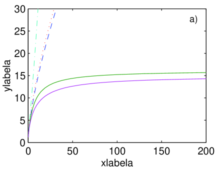
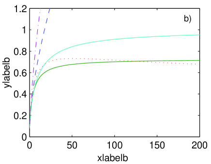
Figure 5: a) The chemical potential as a function of the interaction potential $\tilde{V}_{0}=V_{0}/\hbar\omega\ell_{\rm trap}$ as calculated by the various different models. The solid lines represent the results from the GHFB2 theory (upper line) and the GPE results of the previous section (lower line). The other results correspond to the GHFB1 theory (dashed), HFB-Popov theory (dash-dot) and the BdG equations (dotted). b) The chemical potential per atom in the system as a function of $V_{0}$. The exact results predict that $\mu/N_{\rm tot}\hbar\omega=1$ in the high $V_{0}$ limit. The broken lines correspond to the same curves as in part (a), while the solid lines swap - the lower curve representing the GHFB2 results in this figure. The parameter $\gamma_{\rm trap}$ is not plotted, however for comparison purposes $\tilde{V}_{0}=200$ roughly corresponds to $\gamma_{\rm trap}\approx 80$.

In terms of the chemical potential, neither the BdG nor the HFB-Popov models give the required behaviour, instead $\mu$ increases rapidly as $V_{0}$ is increased. In neither model does the graph show a plateau in the high-$V_{0}$ limit, and the chemical potential greatly exceeds the Tonks-Girardeau limit $\mu=N_{\rm tot}\hbar\omega$ in the HFB-Popov case. Instead the chemical potential roughly follows the $V_{0}^{2/3}$ behaviour for all $V_{0}$. The differences between these two models is seen in Fig. 5b, in which the results differ due to the different total populations. In the BdG case the non-condensate population increases very rapidly, such that in the very high-$V_{0}$ limit $\mu/N_{\rm tot}$ is actually decreasing. In the HFB-Popov model, the interactions between the condensate and non-condensate slow the growth of the non-condensate population, but the chemical potential still rises unchecked.

The disagreement of these models with the exact results is not at all surprising. In both models the anomalous average is completely neglected, and so the many-body T-matrix is not introduced at all. We have argued here, and in earlier papers Lee et al. (2002); Lee and Morgan (2002), about the importance of many-body effects in interactions in low-dimensions, and so we expect that neglecting these effects will lead to an inadequate theory. The BdG and HFB-Popov results presented here are similar to those obtained in the homogeneous gas by Lieb and Liniger Lieb and Liniger (1963), who found that the standard Bogoliubov method failed at high interaction strengths, when $\gamma\gtrsim 2$. In our results we also see quite good agreement with the GPE of the previous section for $\gamma_{\rm trap}\lesssim 1$ and the differences between the theories become much greater when $\gamma_{\rm trap}$ is increased above this point . Note that $\gamma_{\rm trap}\sim 2$ corresponds to $\tilde{V}_{0}\sim 10$ in the figure, which is roughly the point at which the curves separate.

The anomalous average, and therefore the many-body T-matrix, can first be included by solving the GHFB1 equations. Figure 5 shows that there is little difference between these results and those of the HFB-Popov theory. The chemical potential still easily exceeds the limit of the Tonks-Girardeau gas, and so the GHFB1 theory also fails rapidly as $V_{0}$ increases.

However, the GHFB1 results do allow us to examine the form of the many-body T-matrix. In Fig. 6 the spatial dependence of the many-body T-matrix is plotted as $V_{0}$ is increased. In fact, the value being plotted is the T-matrix divided by the condensate density $|\psi(x)|^{2}$. From the previous section we expect that the T-matrix becomes proportional to the condensate density as $V_{0}\rightarrow\infty$, as in Eq. (16). Figure 6 shows that as the interaction strength is increased this becomes an increasingly good approximation. The very good agreement with the form expected for large $V_{0}$ is further evidence that the coupling parameter $g_{\rm LL}(x)$ derived earlier is accurate in this limit. This verifies our approximation for the many-body T-matrix in terms of the off-shell two-body T-matrix numerically.

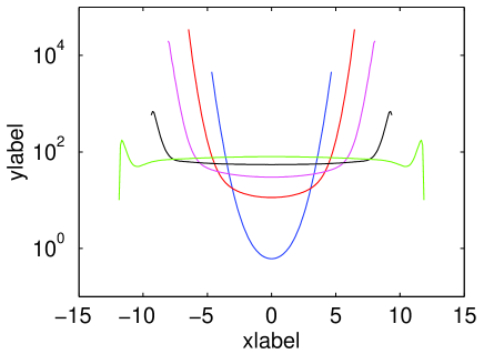
Figure 6: $T_{\rm MB}(x)/N_{0}|\psi(x)|^{2}$ for the many-body T-matrix calculated from the GHFB1 theory for various values of $V_{0}$. Note that the ratio is only plotted for the range over which the condensate density is significant. The values of $\tilde{V}_{0}$ used were $0.2$, $2.4$, $6.5$, $15$ and $44$, which correspond to the narrowest to the widest curves respectively. These values correspond to $\gamma_{\rm trap}=0.02$, $0.46$, $1.6$, $4.3$ and $16.5$.

That the GHFB1 theory fails in the high-$V_{0}$ limit is not particularly surprising. In the low-$V_{0}$ limit almost all the atoms are in the condensate. As the interaction strength is increased, however, we reach the regime of the quasicondensate discussed by Petrov et al. Petrov et al. (2000). As $V_{0}$ is increased the number of atoms in excited states (i.e. $\rho$) increases, and can become a sizable proportion of the total number of atoms in the system. It therefore becomes important to describe the interactions between these atoms accurately.

The description of interactions between excited atoms is more complicated than those between condensate atoms. However, two limits may be investigated relatively straightforwardly. If the majority of the collisions occur at a high energy then the correct description would be given by the two-body T-matrix (since the many-body T-matrix tends towards the two-body T-matrix in this limit). On the other hand, if the majority of the collisions are at low energy, then it is more appropriate to describe them by the same many-body T-matrix as used to treat the condensate-condensate interactions. In 2D and 3D it might be expected that the large density of states at high energies should mean that the majority of collisions are in this regime. However, in 1D the density of states is independent of energy in a trap. In the zero-temperature limit in which we are working it therefore seems probable that the appropriate description of the interactions involving non-condensate atoms is the same many-body T-matrix used to describe the condensate interactions.

The many-body T-matrix is used to describe non-condensate interactions in the GHFB2 version of the theory. It can be seen from Fig. 5 that the results using this theory are quite different from those of the GHFB1 theory. In the low-$V_{0}$ limit the results are similar, but as the interactions are increased the chemical potential becomes independent of $V_{0}$, as we expect in the Tonks-Girardeau limit. The figure clearly shows that it reaches an asymptotic value of $\sim 0.7N_{\rm tot}\hbar\omega$. This is lower than the expected value of $N_{\rm tot}\hbar\omega$, but nonetheless the results are in qualitative agreement with the behaviour expected for the Tonks gas.

Again, we can compare the spatial shape of the many-body T-matrix with our earlier approximation, and the results look essentially the same as those calculated from the GHFB1 results (Fig. 6). The major change in the GHFB2 theory is therefore to provide a better description of the condensate-non-condensate interactions rather than any implicit change in the form of the many-body T-matrix.

We can also compare the predicted density distribution in the high-$V_{0}$ limit with the solutions of the quintic GPE which was shown to give good agreement with the Tonks-Girardeau results in section III. In Fig. 7 we compare the total densities $[N_{0}|\psi(x)|^{2}+\rho(x)]$ for the different models with the Thomas-Fermi prediction from Eq. (18). It can easily be seen that the best agreement is given by the GHFB2 theory, while the BdG, HFB-Popov and GHFB1 results all give entirely the wrong shape. It must be said however, that the GHFB2 results are still not in good agreement with the predicted density.

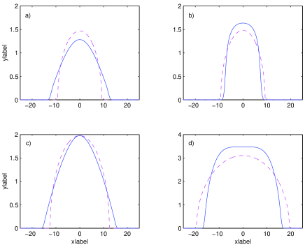
Figure 7: Total density $N_{0}|\psi(x)|^{2}+\rho(x)$ (solid) compared to the Quintic GPE prediction in the Thomas-Fermi limit (dashed) in the high $V_{0}$ regime for the different theories. a) GHFB1 results at $\tilde{V}_{0}=50$ ($\gamma_{\rm trap}=20$) (this was as high a potential for which consistent results were obtained). b) GHFB2 results at $\tilde{V}_{0}=100$ ($\gamma_{\rm trap}=30$). c) HFB-Popov results at $\tilde{V}_{0}=20$ ($\gamma_{\rm trap}=5$) (again, results for potentials higher than this were not obtained). d) The BdG equation results at $\tilde{V}_{0}=100$ ($\gamma_{\rm trap}=15$).

Thus the GHFB2 theory interpreted in the normal manner fails to quantitatively describe the 1D system in the impenetrable limit. This is not surprising since it assumes the existence of a condensate while we know that a condensate does not exist in this limit. Nevertheless, the GHFB2 theory does give qualitatively the correct behaviour for the chemical potential and density in the high-$V_{0}$ limit, which is a significant improvement on the other forms of mean-field theory used for 3D condensates.

The failure of the GHFB1 theory and the relative success of the GHFB2 theory indicate that the description of the non-condensate is the key to solving the 1D problem in the strongly-interacting limit. The GHFB1 model fails at high $V_{0}$ since an increase in $V_{0}$ leads to an increase in $\rho$. The $\rho$ term obviously becomes far too dominant in GHFB1 and therefore needs to be suppressed by some means. In GHFB2 the many-body T-matrix is introduced to describe interactions involving $\rho$, and since $T_{\rm MB}/V_{0}$ decreases with increasing $V_{0}$ this achieves the required suppression. As confirmation of this argument, the GHFB1 results were rerun with $\rho$ artificially set to zero. With this adjustment, the GHFB1 model gave results which looked qualitatively similar to the GHFB2 results, with the chemical potential reaching a plateau in the high-$V_{0}$ limit.

IV.2 Quasiparticle spectrum

Having seen qualitative agreement between the GHFB2 theory and the expected behaviour of the chemical potential and the density, we turn now to investigate the quasiparticle spectrum. In the high-energy limit the quasiparticles are predicted to be single-particle like, and therefore for a 1D harmonic potential the energy will rise linearly with the quasiparticle quantum number. However, for the low-energy quasiparticle states (with energies less than $\sim\mu$), we can use the hydrodynamic theory to obtain an expression for the quasiparticle energies $\varepsilon_{n}$ in the Thomas-Fermi limit Stringari (1996). Using the same method as in Stringari (1996), we find that the low-energy quasiparticle spectrum for a BEC in 1D described by a cubic GPE is

$$\varepsilon_{n}=\hbar\omega\sqrt{{n(n+1)\over 2}},$$ (30)

where $n=1,2,...$ and $n=1$ is the Kohn mode. However, we have shown earlier that in the impenetrable limit the system is described instead by a quintic GPE. For such a GPE the same hydrodynamic approach instead predicts Minguzzi et al. (2001)

$$\varepsilon_{n}=n\hbar\omega,$$ (31)

which is obviously what one would expect for non-interacting fermions, and so we would expect this relationship from a correct theory in the high-$V_{0}$ limit.

Figure 8 shows the GHFB2 results for the energies of the first four quasiparticle modes as a function of the interaction strength. In the weakly-interacting limit the energies are all close to the prediction of Eq. (30), as expected. However, as the interaction strength is increased, the quasiparticle energies do not go over to the limit of Eq. (31). Instead they all fall to around 60% of that value and, even in the high-$V_{0}$ limit, the relationship between the different energies scales more like Eq. (30) than Eq. (31). The conclusion which must be drawn is that the GHFB2 theory does not predict the quasiparticle energies at all accurately in the high-$V_{0}$ limit. This can be seen particularly strongly in the case of the Kohn mode ($\varepsilon_{1}$), which should be equal to $\hbar\omega$ at all interaction potentials since it simply corresponds to a centre-of-mass oscillation of the entire system in the harmonic potential.

The reason that GHFB2 does not predict the quasiparticle spectrum well is because it does not include any dynamics of the non-condensate. In the strongly-interacting limit a large proportion of the atoms in the system are in the non-condensate, which is assumed to be completely static in all of the theories discussed here. Since the Kohn mode corresponds to the motion of all of the atoms together, it is not surprising that a model which does not include the dynamics of a large proportion of those atoms predicts the wrong frequency.

To see this in more detail, all of the theories discussed here can be derived by starting from the generalised time-dependent GPE

$$i\hbar{\partial\Psi(x,t)\over\partial t}=$$ (32)

$$-{\hbar^{2}\over 2m}{\partial^{2}\over\partial x^{2}}\Psi(x,t)+N_{0}U_{\rm con}(x)|\Psi(x,t)|^{2}\Psi(x,t)$$

$$\mbox{}+V_{\rm trap}(x)\Psi(x,t)+2U_{\rm ex}(x)\rho(x)\Psi(x,t),$$

and expanding $\Psi(x,t)$ in terms of the unperturbed ground-state $\psi(x)$ and time-dependent fluctuations $\Delta\psi(x,t)$, and linearising (see, for example, Ruprecht et al. (1996)). The trouble occurs when it is recognised that in 1D the appropriate coupling parameter $U_{\rm con}(x)$ is the many-body T-matrix, as argued earlier. In the high-$V_{0}$ limit, the many-body T-matrix is proportional to $N_{0}|\psi(x)|^{2}$ in the static case as we have shown. Applying the local density approximation, the time-dependent form of the many-body T-matrix should then be $N_{0}|\Psi(x,t)|^{2}$ (assuming that the time-scale for interparticle interactions is much quicker than that for condensate dynamics). In the linearisation procedure, one should therefore also expand the many-body T-matrix as

$$T_{\rm MB}(x)\propto|\psi(x)+\Delta\psi(x,t)|^{2}.$$ (33)

Making this replacement for $U_{\rm con}(x)$ in Eq. (32) while setting $\rho=0$ leads directly to the quintic GPE discussed earlier and hence to the result of Eq. (31). We see therefore that including the dynamics of the anomalous average in the GHFB2 theory will lead to the correct prediction for the excitation spectrum in the high-$V_{0}$ limit. For a general value of $V_{0}$, including the fluctuations of the many-body T-matrix requires a dynamic treatment of the anomalous average and hence of the non-condensate generally.

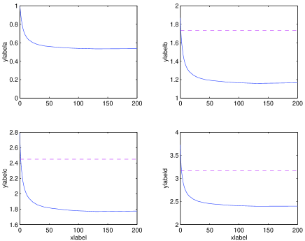
Figure 8: The energies of the first four quasiparticle states as a function of the interaction potential $\tilde{V}_{0}$, as predicted by GHFB2 theory. The dashed lines indicate the value expected from hydrodynamic theory by the linearisation of the cubic GPE (for the Kohn mode [$\varepsilon_{1}$] the expected value is $1\hbar\omega$). The correct values in the high-$V_{0}$ limit are $\hbar\omega$, $2\hbar\omega$, $3\hbar\omega$, and $4\hbar\omega$ (from left to right).

IV.3 Coherences

It is of interest to calculate the coherence functions for the Lieb-Liniger gas from the GHFB2 results. We have argued that we are dealing with a gas in which a condensate may form in the low-$V_{0}$ limit, but where it disappears when the interactions are increased. Since coherence is a major feature of a condensate we should be able to see a loss of coherence as $V_{0}$ is increased, and again we can try to relate this to the expected results in the Tonks limit.

IV.3.1 First-order coherence

The first order coherence function $G^{(1)}({\bf r},{\bf r}^{\prime})$ is defined in terms of the quantum field operators by Naraschewski and Glauber (1999)

$$G^{(1)}({\bf r},{\bf r}^{\prime})=\langle\hat{\Psi}^{\dagger}({\bf r})\hat{\Psi}({\bf r}^{\prime})\rangle,$$ (34)

and the normalised first order coherence function is therefore

$$g^{(1)}({\bf r},{\bf r}^{\prime})={G^{(1)}({\bf r},{\bf r}^{\prime})\over\sqrt{G^{(1)}({\bf r},{\bf r})G^{(1)}({\bf r}^{\prime},{\bf r}^{\prime})}}.$$ (35)

Decomposing the field operator in terms of the condensate and its fluctuations leads to an expression for the coherence function at $T=0$ in terms of the condensate wave function and Bogoliubov quasiparticle amplitudes Dodd (1997)

$$G^{(1)}({\bf r},{\bf r}^{\prime})=N_{0}\psi_{0}^{*}({\bf r})\psi_{0}({\bf r}^{\prime})+\sum_{i\neq 0}v_{i}({\bf r})v_{i}^{*}({\bf r}^{\prime}).$$ (36)

Figure 9 shows the normalised first order coherence function obtained from the GHFB2 results for various values of $V_{0}$. Note that the figure has been plotted in terms of the distance scale $\tilde{x}=x/R_{\rm TF}$, where $R_{\rm TF}$ is the Thomas-Fermi radius of the condensate, in order to take into account the greater spatial extent of a condensate with stronger interactions. Figure 9 clearly shows that the system is coherent over its entire length in the weakly-interacting limit. However, as the interaction strength is increased the coherence can be seen to diminish substantially, and the width of the central maximum decreases as well. A diminishing range of coherence is consistent with the absence of a true condensate in the strongly-interacting regime. However, the rate at which the coherence calculated here decreases is surprisingly slow. Gangardt and Shlyapnikov Gangardt and Shlyapnikov (2002) have presented results for the coherence function obtained from hydrodynamic theory applied to a 1D gas, and they see a much greater fall in the range of the coherence length - dropping by almost an order of magnitude as $\gamma_{\rm trap}$ decreases from $0.1$ to $10$. However, their results were obtained for a system of $10^{4}$ atoms, many more than we deal with here. Also, even for the largest value of $V_{0}$ plotted, the condensate depletion is still only about $50$%, in our case.

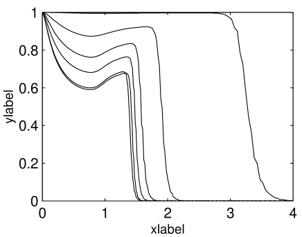
Figure 9: The normalised first order coherence function $g^{(1)}(0,x)$ calculated using the GHFB2 theory for various values of $V_{0}$. The solid curves represent (from top to bottom) the results for $\tilde{V}_{0}=0.2,2.4,6.5,15,100$ and $200$ (corresponding to $\gamma_{\rm trap}=0.02,0.46,1.6,4.1,31$ and $61$ respectively). The coherence function is plotted as a function of $x/R_{\rm TF}$ where $R_{\rm TF}$ is the Thomas-Fermi radius of the condensate.

IV.3.2 Second-order coherence

We now look briefly at the second-order coherence function defined by Naraschewski and Glauber (1999)

$$g^{(2)}({\bf r},{\bf r}^{\prime})={\langle\hat{\Psi}^{\dagger}({\bf r})\hat{\Psi}^{\dagger}({\bf r}^{\prime})\hat{\Psi}({\bf r}^{\prime})\hat{\Psi}({\bf r})\rangle\over\langle\hat{\Psi}^{\dagger}({\bf r})\hat{\Psi}({\bf r})\rangle\langle\hat{\Psi}^{\dagger}({\bf r}^{\prime})\hat{\Psi}({\bf r}^{\prime})\rangle}.$$ (37)

We will consider this function only in the equal-position limit (i.e. when ${\bf r}={\bf r}^{\prime}$), in which case it may be written as

$$g^{(2)}(x,x)=$$

$$1+{2N_{0}|\psi(x)|^{2}[\rho(x)+\kappa(x)]+|\rho(x)|^{2}+|\kappa(x)|^{2}\over\left[N_{0}|\psi(x)|^{2}+\rho(x)\right]^{2}},$$

following a similar argument as for the first-order coherence function. The second-order equal-position coherence function is of interest because of the various limits in which exact results are known. For a pure BEC with perfect second-order coherence we have $g^{(2)}(x,x)=1$, whilst for a thermal cloud of bosons $g^{(2)}(x,x)=2$ Dodd et al. (1997); Naraschewski and Glauber (1999). In the strong-coupling limit in 1D however, the Bose-Fermi mapping theorem predicts that $g^{(2)}(x,x)=0$ Girardeau et al. (2001) for impenetrable bosons. We would therefore expect to find a second-order coherence of close to $1$ in the weakly-interacting limit, which decreases to $0$ as the interaction strength is increased, in contrast to the higher dimensional case where the coherence function would increase to $2$ as the non-condensate became significant .

Figure 10 shows $g^{(2)}(x,x)$ as calculated from the results of the GHFB2 theory. The results can be seen to be close to unity, as expected, for the weakly-interacting case (and rising to $2$ outside the region where the condensate exists). As the interactions are increased, $g^{(2)}(x,x)$ initially decreases closer to the $g^{(2)}(x,x)=0$ limit expected. However, in the very strongly-interacting limit the coherence function rises again to become greater than $1$. Thus the GHFB2 theory, whilst in qualitative agreement with the behaviour of the chemical potential and the density, does not give the expected results for the coherence of the system in the impenetrable limit.

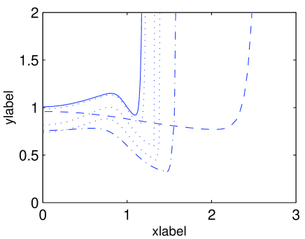
Figure 10: Plot of the normalised equal-position second-order coherence function $g^{(2)}(x,x)$ obtained from the results of GHFB2 theory for various values of $V_{0}$. The dashed line shows the weakly interacting limit with $\tilde{V}_{0}=0.2$, the dot-dashed line is for $\tilde{V}_{0}=2.4$. The dotted lines then correspond to values of $\tilde{V}_{0}=6.5,15,100$ from bottom to top, and the final solid line is in the strongly interacting limit with $\tilde{V}_{0}=200$ (these values correspond to $\gamma_{\rm trap}=0.02,0.46,1.6,4.1,31$ and $61$ respectively). Note that the $x$-axis is scaled in units of the Thomas-Fermi radius of the system.

V Reinterpreting the results

As seen in the previous section, although the GHFB2 theory seems to go further than other standard theories in describing the 1D Bose gas into the strongly-interacting limit, there are significant differences between the results in the impenetrable limit and the exact results of the Tonks-Girardeau gas. However, we will see in this section that the agreement can be improved significantly by reinterpreting the results in a different manner. The disagreement with the expected values for the asymptotic value of the chemical potential and with the shape of the density are both related to the non-condensate population in the form of $\rho(x)$. Looking again at Fig. 5 one can see that the chemical potential in the GHFB2 case rises to an asymptotic value of approximately $15\hbar\omega$. Although this result was obtained for a condensate population of $N_{0}=15$, it is in excellent agreement with the expected result for a system with $15$ atoms in total. By itself this may appear to be a co-incidence; however the shape of the density resulting merely from the condensate “wave function” $\psi(x)$ is plotted against the Thomas-Fermi exact prediction in Fig. 11, and the two shapes can be seen to agree quite well. It seems that the best agreement would be midway between that in Fig. 11, and that in Fig. 7b (where the total density has been plotted).

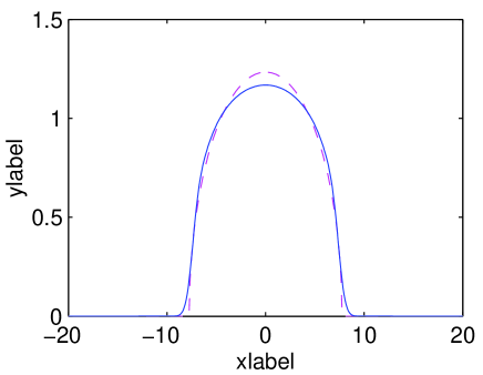
Figure 11: Density due to the condensate population only (solid) resulting from the GHFB2 theory at $\tilde{V}_{0}=100$ ($\gamma_{\rm trap}=30$). The dashed line again shows the Thomas-Fermi prediction for the exact density for $15$ atoms in the Tonks-Girardeau limit.

This seems to imply that the GHFB2 theory predicts the correct results in the strongly-interacting limit if one partly ignores the contributions from the non-condensate (these contributions are sizeable - the non-condensate population for the results plotted in Fig. 11 is about $N_{0}/2$). This would have to be combined with a re-interpretation of the condensate density as the quasi-condensate density and, ultimately, as the total density. Some procedure of this kind is clearly required in 1D because the various theories discussed in the previous section are based on the existence of a condensate whereas in fact the condensate disappears as $V_{0}$ increases.

As another illustration of the good agreement with exact results which can be obtained with such a reinterpretation, in Fig. 12 the second-order equal-position coherence function is plotted with results obtained from the GHFB1 theory with $\rho(x)$ artificially set to zero (as mentioned earlier, this approach gave qualitative agreement with the expected behaviour of the chemical potential). The results in this case clearly show the behaviour predicted in the previous section, with $g^{(2)}(x,x)$ decreasing from unity to zero as the interaction strength is increased. Such a theory (with $\rho(x)=0$) would result from a reinterpretation of $N_{0}|\psi(x)|^{2}$ as the total density of the system, rather than merely that of the condensate. The agreement with the expected behaviour for $g^{(2)}(x,x)$ can easily be seen from the following argument. In the high-$V_{0}$ limit we have shown that $T_{\rm MB}$ becomes independent of $V_{0}$. From Eq. (29), this must mean that $\kappa(x)\rightarrow-N_{0}\psi_{0}^{2}(x)$ in the same limit. Equation (IV.3.2) then clearly shows that the second order coherence function vanishes in the high-$V_{0}$ limit if $\rho=0$.

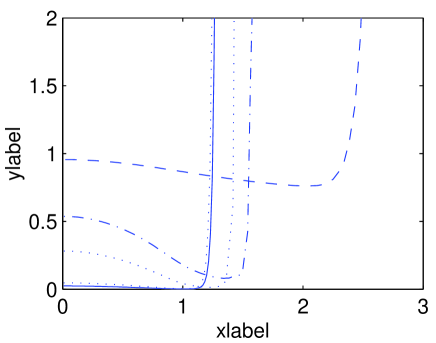
Figure 12: Plot of the normalised equal-position second-order coherence function $g^{(2)}(x,x)$ obtained from the results of GHFB1 theory with $\rho(x)$ artificially set to zero everywhere, for various values of $V_{0}$. The dashed line shows the weakly interacting limit with $\tilde{V}_{0}=0.2$, the dot-dashed line is for $\tilde{V}_{0}=3$. The dotted lines then correspond to values of $\tilde{V}_{0}=7.5$ and $32$, while the final solid line is in the strongly interacting limit with $\tilde{V}_{0}=48$ (these values correspond to $\gamma_{\rm trap}=0.02,0.65,2.1,11$ and $17$ respectively). Note that the $x$-axis is scaled in units of the Thomas-Fermi radius of the system.

That such a reinterpretation of the condensate is necessary and will lead to the correct mean-field theory at large $V_{0}$ can be seen by comparison with the GPE results in section III.3. If we set $\rho=0$ and reinterpret $n_{0}(x)$ as $n_{\rm tot}(x)$ then the GHFB theory reduces to the earlier GPE theory, the only difference being that $g_{\rm 1D}(x)$ is calculated from Eq. (29) instead of Eq. (III.3). Assuming the validity of the local density approximation, however, these two definitions will lead to the same results. We note that a theory has recently been proposed by Anderson et al. Andersen et al. (2002); Khawaja et al. (2002) which in effect leads to a similar reinterpretation of the quantities $\rho(x)$, $\kappa(x)$ and $n_{0}(x)$ by considering the effects of phase fluctuations to all orders, and this approach may provide a microscopic justification for this procedure.

VI Conclusions

In this paper we have given a form for an approximate many-body T-matrix to describe the scattering which occurs in a zero temperature 1D Bose gas. This approximate T-matrix enables the 1D Bose system to be described by a Gross-Pitaevskii equation which is easily solved. We have shown that the solutions to this equation for a trapped system are in excellent agreement with the density of a 1D Lieb-Liniger model gas in the two limits in which exact results are known, and that the density distribution of such a gas changes markedly as the interactions become stronger.

We have also attempted to push various higher-order theories of BECs from the weakly-interacting regime into the strongly-interacting regime for the Lieb-Liniger gas. We have shown that the theories which neglect many-body effects on the interactions (BdG and HFB-Popov) fail to provide adequate results at even quite low interaction strengths. The GHFB1 theory includes the many-body T-matrix for condensate interactions, but it also fails to describe the strongly-interacting limit since it does not account for the condensate-non-condensate interactions properly and hence the terms involving $\rho$ become too large.

However, the GHFB2 theory, which includes many-body effects in the condensate-non-condensate interactions, gave results which were qualitatively correct even in the strongly-interacting limit, predicting the correct behaviour of the chemical potential and density profile. Quantitative agreement was not found, but the results show that GHFB2 describes the strongly-interacting limit to a much better degree than the other mean-field theories tested.

GHFB2 theory still fails to adequately describe some aspects of the system however. The first-order coherence function shows qualitatively the behaviour expected, but the second-order coherence, while initially showing the correct behaviour in the low- to mid-$V_{0}$ range, deviates from the expected limit at high-$V_{0}$. Furthermore, the quasiparticle excitation spectrum does not go over to the correct behaviour at high-$V_{0}$.

The quasiparticle spectrum can be corrected if the theory is modified to allow for fluctuations in the many-body T-matrix, as well as in the condensate density. This requires a dynamical treatment of the non-condensate. At the same time, it seems that the key to pushing the GHFB2 theory into the high-$V_{0}$ limit (obtaining the correct coherences and quantitative agreement in general) lies in a reinterpretation of the non-condensate density as the total density, and we have presented some heuristic evidence that this will lead to the expected results.

Appendix A The many-body T-matrix in 3D

As an illustration of our approximation of the many-body T-matrix in terms of the off-shell two-body T-matrix, we show in this appendix that in the three-dimensional case it reproduces the known results for the many-body T-matrix.

The 3D case differs from 1D and 2D because the many-body T-matrix is only a small correction to the two-body T-matrix. As mentioned earlier, the 3D two-body T-matrix is a constant $U_{0}=4\pi\hbar^{2}a/m$ to first order in the low-energy limit. The first approximation to the 3D coupling parameter is therefore $g_{\rm 3D}=U_{0}$. We can then ask if the method used in this paper for 1D (and used in reference Lee et al. (2002) for 2D) accurately predicts the effects of the medium on the scattering.

In Lee et al. (2002) we showed that our approximation for the many-body T-matrix in 3D is

$$g_{\rm 3D}=\langle 0|T_{\rm MB}(E=0)|0\rangle\approx\langle 0|T_{\rm 2B}(E=-{16\over\pi^{2}}\mu)|0\rangle,$$ (39)

and the off-shell two-body T-matrix for a gas of hard-spheres of radius $a$ was shown in Morgan et al. (2002) to be

$$\langle{\bf 0}|T_{\rm 2B}^{\rm 3D}(E)|{\bf 0}\rangle=$$ (42)

$$\left\{\begin{array}[]{ll}U_{0}\left[1-i\sqrt{mE\over\hbar^{2}}a-\frac{1}{3}{mE\over\hbar^{2}}a^{2}\right],&\mbox{for }E>0,\\ U_{0}\left[1+\sqrt{m|E|\over\hbar^{2}}a-\frac{1}{3}{mE\over\hbar^{2}}a^{2}\right],&\mbox{for }E<0,\end{array}\right.$$

Combining these equations gives (to first order in the small parameter $k_{\mu}a=\sqrt{m\mu a^{2}/\hbar^{2}}$)

$$g_{\rm 3D}=U_{0}\left[1+\left({16\mu ma^{2}\over\pi^{2}\hbar^{2}}\right)^{1/2}\right]+\mbox{O}[(k_{\mu}a)^{2}].$$ (43)

We can rewrite this in terms of the density $n_{0}$, since in a homogeneous system $\mu=g_{\rm 3D}n_{0}$ to leading order. Making this substitution and solving for $g_{\rm 3D}$ gives the result

$$g_{\rm 3D}=U_{0}\left[1+{8\over\sqrt{\pi}}(n_{0}a^{3})^{1/2}\right]+\mbox{O}(n_{0}a^{3}),$$ (44)

where we have expanded in terms of the dilute gas parameter $n_{0}a^{3}$, which is small for a dilute gas BEC. This result agrees with other solutions Shi and Griffin (1998); Morgan (1999) for the many-body T-matrix in 3D homogeneous systems. At $T=0$ we can, therefore, account for many-body effects on particle scattering using an off-shell two-body T-matrix.

References

- Görlitz et al. (2001) A. Görlitz, J. M. Vogels, A. E. Leanhardt, C. Raman, T. L. Gustavson, J. R. Abo-Shaeer, A. P. Chikkatur, S. Gupta, S. Inouye, T. Rosenband, et al., Phys. Rev. Lett. 87, 130402 (2001).
- Schreck et al. (2001) F. Schreck, L. Khaykovich, K. L. Corwin, G. Ferrari, T. Bourdel, J. Cubizolles, and C. Salomon, Phys. Rev. Lett. 87, 080403 (2001).
- Girardeau (1960) M. Girardeau, J. Math. Phys. 1, 516 (1960).
- Lieb and Liniger (1963) E. H. Lieb and W. Liniger, Phys. Rev. 130, 1605 (1963).
- Lieb (1963) E. H. Lieb, Phys. Rev. 130, 1616 (1963).
- Lee et al. (2002) M. D. Lee, S. A. Morgan, M. J. Davis, and K. Burnett, Phys. Rev. A 65, 043617 (2002).
- Hohenberg (1967) P. C. Hohenberg, Phys. Rev. 158, 383 (1967).
- Pitaevskii and Stringari (1991) L. Pitaevskii and S. Stringari, J. Low Temp. Phys. 85, 377 (1991).
- Ketterle and van Druten (1996) W. Ketterle and N. van Druten, Phys. Rev. A 54, 656 (1996).
- Petrov et al. (2000) D. S. Petrov, G. V. Shlyapnikov, and J. Walraven, Phys. Rev. Lett. 85, 3745 (2000).
- Schwartz (1977) M. Schwartz, Phys. Rev. B 15, 1399 (1977).
- Tonks (1936) L. Tonks, Phys. Rev. 50, 955 (1936).
- Girardeau et al. (2001) M. D. Girardeau, E. M. Wright, and J. M. Triscari, Phys. Rev. A 63, 033601 (2001).
- Morgan (2000) S. A. Morgan, J. Phys. B 33, 3847 (2000).
- Morgan et al. (2002) S. A. Morgan, M. D. Lee, and K. Burnett, Phys. Rev. A 65, 022706 (2002).
- Lee and Morgan (2002) M. D. Lee and S. A. Morgan, J. Phys. B 35, 3009 (2002).
- Stoof et al. (1996) H. T. C. Stoof, M. Bijlsma, and M. Houbiers, J. Res. Natl. Inst. Stand. Technol. 101, 443 (1996).
- Bijlsma and Stoof (1997) M. Bijlsma and H. T. C. Stoof, Phys. Rev. A 55, 498 (1997).
- Proukakis et al. (1998) N. P. Proukakis, S. A. Morgan, S. Choi, and K. Burnett, Phys. Rev. A 58, 2435 (1998).
- Kolomeisky et al. (2000) E. B. Kolomeisky, T. J. Newman, J. P. Straley, and X. Qi, Phys. Rev. Lett. 85, 1146 (2000).
- Kolomeisky and Straley (1992) E. B. Kolomeisky and J. P. Straley, Phys. Rev. B 46, 11749 (1992).
- Olshanii (1998) M. Olshanii, Phys. Rev. Lett. 81, 938 (1998).
- Dunjko et al. (2001) V. Dunjko, V. Lorent, and M. Olshanii, Phys. Rev. Lett. 86, 5413 (2001).
- Bergeman et al. (2002) T. Bergeman, M. Moore, and M. Olshanii, preprint, cond-mat/0210556 (2002).
- Hutchinson et al. (2000) D. A. W. Hutchinson, K. Burnett, R. J. Dodd, S. A. Morgan, M. Rusch, E. Zaremba, N. P. Proukakis, A. Griffin, M. Edwards, and C. W. Clark, J. Phys. B 33, 3825 (2000).
- Stringari (1996) S. Stringari, Phys. Rev. Lett. 77, 2360 (1996).
- Minguzzi et al. (2001) A. Minguzzi, P. Vignolo, M. L. Chiofalo, and M. P. Tosi, Phys. Rev. A 64, 033605 (2001).
- Ruprecht et al. (1996) P. A. Ruprecht, M. Edwards, K. Burnett, and C. W. Clark, Phys. Rev. A 54, 4178 (1996).
- Naraschewski and Glauber (1999) M. Naraschewski and R. J. Glauber, Phys. Rev. A 59, 4595 (1999).
- Dodd (1997) R. Dodd, Ph.D. thesis, University of Maryland (1997).
- Gangardt and Shlyapnikov (2002) D. Gangardt and G. Shlyapnikov, preprint, cond-mat/0207338 (2002).
- Dodd et al. (1997) R. J. Dodd, C. W. Clark, M. Edwards, and K. Burnett, Opt. Express 1, 284 (1997).
- Andersen et al. (2002) J. O. Andersen, U. A. Khawaja, and H. T. C. Stoof, Phys. Rev. Lett. 88, 070407 (2002).
- Khawaja et al. (2002) U. A. Khawaja, J. Andersen, N. Proukakis, and H. Stoof, Phys. Rev. A 66, 013615 (2002), [See also the erratum: cond-mat/0209120].
- Shi and Griffin (1998) H. Shi and A. Griffin, Phys. Rep. 304, 1 (1998).
- Morgan (1999) S. A. Morgan, Ph.D. thesis, University of Oxford (1999).