Resonant scattering of solitons

Abstract

We study the scattering of solitons in the nonlinear Schrödinger equation on local inhomogeneities which may give rise to resonant transmission and reflection. In both cases, we derive resonance conditions for the soliton’s velocity. The analytical predictions are tested numerically in regimes characterized by various time scales. Special attention is paid to intermode interactions and their effect on coherence, decoherence and dephasing of plane-wave modes which build up the soliton.

The scattering of solitons by various scattering centers in the nonlinear Schrödinger equation leads to resonant transmission and reflection if the soliton velocity matches certain resonance conditions. By assuming that the soliton is composed of a weighted superposition of modes (i.e. a wave packet) different scattering regimes are observed depending on the ratio of the duration of the scattering event and the characteristic mode-mode interaction time due to nonlinearity. Resonant transmission does not suffer from mode dephasing, while resonant reflection (Fano resonance) does. Consequently transmission resonances are observed independent of the scattering regime, while the opposite holds for Fano reflection resonances.

I Introduction

Transmission of linear waves through inhomogeneous media is a topic of wide interest psbwzzgp89 ; Klyatskin ; LifGredPast ; Zwerger ; dhgpt99 . In the one-dimensional case, two basic resonant features of wave scattering are known. One of them corresponds to the wave travelling above a barrier or a potential well. Proximity of the wave’s frequency to that of a standing wave captured inside the scattering potential leads to a resonance, i.e., the transmission may be strongly enhanced in a vicinity of the resonance LLIII . In fact, the transmission at resonance is perfect, which is used in Fabry-Perrot interferometers cohen . The connection of the resonant scattering to the Levinson’s theorem and the existence of bound states in potential wells is discussed, e.g., in Ref. LLIII .

Resonant reflection is possible too, as a consequence of the Fano resonance fano , and it occurs whenever a wave may choose between two scattering paths, which finally merge into one exit. Destructive interference may then lead to total reflection. An adequate explanation goes through the coupling of a local Fano state to a continuum gdm93 ; gl93 ; ns94 . The wave may then again either pass directly through the continuum or by visiting the Fano state. The resonance condition is provided directly by the matching of the wave’s frequency to the eigenfrequency of the Fano state. More than one wave paths are typically also generated by time-dependent scattering potentials.

Fano resonances imply the coherence of the wave phases throughout the scattering process, hence any significant dephasing effects will suppress the resonance. At the same time, the resonant transmission mechanism does not rely on phase coherence, therefore dephasing does not destroy it.

Similar situations can also be observed in nonlinear systems which possess continuous or discrete translational invariance. For instance, nonlinear lattice models support time-periodic spatially localized states in the form of discrete breathers breather . If small-amplitude plane waves are sent towards such a breather, it acts as a time-periodic scattering potential. The temporal periodicity of the potential leads to excitation of many new scattering channels, shifted by multiples of the breather’s fundamental frequency relative to the frequency of the incoming wave scattering2 . Even if all the additional channels are closed ones, i.e., they do not match the plane-wave’s frequency, they may generate localized Fano states which resonate with the open channel and thus lead to Fano-resonant backscattering sfaemvfmvf02 . In addition, resonant transmission can also be observed in this case skcbrsm97 .

In this paper we study the transmission properties of small-amplitude solitons (rather than plane linear waves) in the discrete nonlinear Schrödinger (DNLS) equation with two types of scattering centers. The first one is a Fano-defect center, which is an extra level coupled to the DNLS equation at one site of the underlying lattice. This Fano center may actually be a strongly localized discrete breather of the DNLS model sfaemvfmvf02 . The second type is a two-site impurity which gives rise to two bound states. Our goal is to predict resonant backscattering and resonant transmission of the small-amplitude soliton impinging onto these defects. To this end, we consider the soliton as a superposition of plane waves or modes, while the nonlinearity leads to mode-mode interactions, which may or may not cause dephasing effects in the course of the scattering process. We will find values of the velocity of the incident soliton at which the resonant transmission and reflection are possible.

The predicted effects can be observed in any physical system which is modelled by the DNLS equation, the most straightforward ones being arrays of nonlinear optical waveguides. These may be realized as set of parallel cores fabricated on a common substrate Yaron , or a virtual array induced in a photorefractive material illuminated by a set of parallel laser beams Moti .

II Resonances in the scattering of linear waves

Before considering the scattering of solitons, we will set the stage, using two simple models which make it possible to observe resonant transmission and reflection in linear wave scattering. In both cases, we will use the linear discrete Schrödinger equation as the unperturbed system. Later on, we will add nonlinearities to make propagation of solitons possible.

II.1 Resonant transmission

Resonant transmission due to bound states is possible if the scattering potential supports at least one bound state. To be flexible, we take a lattice model which allows for two or one bound states, depending on its parameters:

$$i\dot{\phi}_{n}=C(\phi_{n-1}+\phi_{n+1})+\delta_{n,0}\epsilon_{0}\phi_{n}+\delta_{n,1}\epsilon_{1}\phi_{n}\;.$$ (1)

Here $\phi_{n}$ is the complex scalar dynamical variable at the $n$-th site, a real constant $C$ controls the strength of the inter-site coupling, and two diagonal defects are set at sites $n=0$ and $n=1$ with strengths $\epsilon_{0}$ and $\epsilon_{1}$, respectively. In the absence of the defects, Eq. (1) has exact plane-wave solutions, $\phi_{n}=\mathrm{\exp}\left[i(\omega_{q}t-qn)\right]$, whose frequency satisfies the dispersion relation

$$\omega_{q}=-2C\cos q\,.$$ (2)

To find the transmission coefficient $T$ in the presence of the two diagonal defects, we impose proper boundary conditions and obtain, after some algebra (see, e.g., Ref. BambiHu ), for the case of $\epsilon_{0}=\epsilon_{1}\equiv\epsilon$,

$$T=\frac{4C^{4}\sin^{2}q}{\epsilon^{2}(\epsilon-2C\cos q)^{2}+4C^{4}\sin^{2}q}\;.$$ (3)

Perfect transmission ($T=1$) is possible in the case $\epsilon\leq 2C$ under the resonance condition (at the special value of $q$),

$$q^{\prime}=\cos^{-1}(\epsilon/2C)\;.$$ (4)

For small values of the impurity strength, $\epsilon\ll 2C$, the perfect transmission takes place around $q=\pi/2$. With $\epsilon$ approaching $2C$, the value of $q^{\prime}$ moves towards zero (see Fig.1). At $\epsilon=2C$, the perfect transmission occurs exactly at the edge point of the spectrum, $q^{\prime}=0$, and disappears for larger values of $\epsilon$. Therefore, it is possible to control the location of the resonance by varying the impurity strength $\epsilon$.

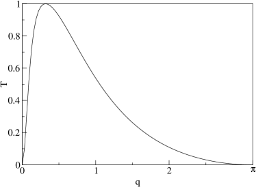
Figure 1: The transmission coefficient $T$ versus $q$ for the case of the resonant transmission, as per Eq. (3) with $C=10$ and $\epsilon=19$.

II.2 Resonant reflection

In order to produce a Fano resonance, we consider the Fano-Anderson model, which amounts to adding an additional local Fano degree of freedom $\varphi$, with the eigenfrequency (energy) $E$, to the linear discrete Schrödinger equation. The dynamical variable $\varphi$ is coupled to the lattice field $\phi_{n}$ at the site $n=0$:

$$i\dot{\phi}_{n} = C(\phi_{n-1}+\phi_{n+1})+\epsilon\varphi\delta_{n0}\;,$$

$$i\dot{\varphi} = -E\varphi+\epsilon\phi_{0}\;.$$ (5)

When $\epsilon=0$, the system decouples into the free wave with the spectrum $\omega_{q}=-2C\cos q$ and an additional localized level with the energy $E$. The value of $E$ is chosen so that it lies inside the continuous spectrum, i.e., $|E|<2C$.

If $\epsilon\neq 0$, the Fano defect interacts with the continuous spectrum locally. To solve the linear system (5), we substitute

$$\phi_{n}=A_{n}\exp\left(i\omega_{q}t\right)\,,\,\varphi=B\exp\left(i\omega_{q}t\right)\,,$$

and obtain

$$-\omega_{q}A_{n} = C(A_{n-1}+A_{n+1})+\epsilon B\delta_{n0}\;,$$

$$-\omega_{q}B = -EB+\epsilon A_{0}\;.$$ (6)

We use the second equation in (6) to eliminate $B$ in favor of $A_{0}$, then the first equation yields

$$-\omega_{q}A_{n}=C(A_{n-1}+A_{n+1})-\epsilon^{2}\left(\omega_{q}-E\right)^{-1}A_{0}\delta_{n0}\;.$$ (7)

Equation (7) amounts to the presence of a resonant scattering potential, which depends on the frequency of the incident wave. Moreover, if the energy of the additional level is located inside the continuous spectrum, $|E|<2C$, as it was assumed above, there is a value $q_{F}=\cos^{-1}\left(-E/2C\right)$ at which the denominator of the last term in Eq. (7) vanishes, according to Eq. (2). At this value of $q$, complete reflection, $T=0$, takes place, as the scattering potential becomes infinitely large.

After some algebra (see, e.g., Ref. BambiHu ), the transmission coefficient $T$ for the linear model based on Eqs. (5) can be written as

$$T=\left[1+\frac{1}{4\sin^{2}q}\frac{\epsilon^{4}}{C^{2}(E-\omega_{q})^{2}}\right]^{-1}\;.$$ (8)

A typical dependence of $T$ versus the incident wavenumber $q$ is shown in Fig. 2 for $E=0$.

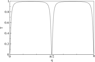
Figure 2: The transmission coefficient as given by Eq. (8), versus the wavenumber $q$ of the inident wave. The parameters are $E=0$, $C=10$ (i.e., $q_{F}=\pi/2$), and $\epsilon=4$.

In the case of $E=0$, the transmission coefficient $T(q)$ vanishes at $q_{F}=\pi/2$. The additional vanishing of $T$ at the band edges $q=0$ and $q=\pi$ is related to the fact that the group velocity of plane waves is equal to zero at these points, and will not be discussed below.

If $\epsilon^{2}/\left(2C^{2}\right)\ll\sin q$, then $T\approx 1$ at all values of $q$ except for close to $q=q_{F}$, as $T(q_{F})=0$. The width of the resonance in the $q$-space is defined by the distance between points at which $T=1/2$, or, as it follows from Eq. (8),

$$\frac{\epsilon^{4}}{4C^{2}(E-\omega_{q})^{2}\sin^{2}q}=1\;.$$ (9)

By expanding $\omega_{q}$ around $q_{F}$, $\omega_{q}\approx\omega_{q_{F}}+\omega_{q}^{\prime}(q_{F})\delta q$, and substituting this into Eq. (9), we find

$$\delta q=\frac{\epsilon^{2}}{4C^{2}\sin^{2}q_{F}}\;.$$ (10)

The width of the resonance is twice the expression (10),

$$\Delta q=\frac{\epsilon^{2}}{2C^{2}\sin^{2}q_{F}}\;.$$ (11)

The above considerations are valid also for the model based on the continuous linear Schrödinger equation augmented with a corresponding $\delta$-like scattering term. Quite a different situation takes place if the local scattering term, added to the linear Schrödinger equation, is nonlinear – in that case, the solution to the scattering problem is not unique, and may be subject to local modulational instability MarkAzbel .

III Soliton scattering

In order to consider a possibility of resonant transmission or reflection in the scattering of a soliton on a local defect, we first add nonlinear terms to the linear Schrödinger equation [see the first equation in the system (5)], thus arriving at the DNLS equation,

$$i\dot{\phi}_{n}=C(\phi_{n-1}+\phi_{n+1})+\lambda|\phi_{n}|^{2}\phi_{n}\;.$$ (12)

Small-amplitude (hence, broad) moving solitons in Eq. (12) are approximated well by the corresponding solution to the continuous NLS equation,

$$\phi_{n}(t) \approx \frac{\eta}{2}\sqrt{\frac{\lambda}{2C}}\mathrm{\exp}\left[i(\frac{V}{2C}n-(\omega_{s}+2)Ct)\right]\times$$ (13)

$$\mathrm{sech}\left[\frac{\eta\lambda}{4C}(n-Vt)\right],$$

where $V$ is the velocity of the soliton, $\omega_{s}=\left(4C^{2}\right)^{-1}(V^{2}-\eta^{2}\lambda^{2}/4)$ is its intrinsic frequency, and $\eta$ is the amplitude yskbam89 .

The velocity $V$ determines a central wavenumber of the soliton’s Fourier transform,

$$q_{c}=V/\left(2C\right)\,.$$ (14)

The soliton may be considered as a superposition of linear plane waves with wavenumbers taking values in an interval around $q_{c}$, the width of this interval being

$$\Delta q_{c}=\ln\left(2+\sqrt{3}\right)\frac{\eta\lambda}{\pi C}\;.$$ (15)

This spectral width is to be compared with the width of the corresponding resonances [e.g., with the expression (11)].

There are two characteristic time scales, which describe the scattering of the soliton (13) by the resonant defect. One of them is the time of the soliton-defect interaction, which is estimated as the soliton’s width $1/\Delta q_{c}$ in the coordinate space, divided by its velocity:

$$\tau_{\mathrm{int}}=\left(\Delta q_{c}V\right)^{-1}\;.$$ (16)

The interaction between waves composing the free soliton defines the second time scale. It can be estimated as the time of dispersion of the wave packet (13) in the linearized equation (12), with $\lambda=0$, which yields, similar to Eq. (16), a result

$$\tau_{\mathrm{disp}}=\left(\Delta q_{c}\Delta v_{g}\right)^{-1}\;,$$ (17)

where $v_{g}(q)=2C\sin q$ is a group velocity of the waves, and

$$\Delta v_{g}=v_{g}(q_{c}+\Delta q_{c}/2)-v_{g}(q_{s}-\Delta q_{c}/2)=4\sin\left(\Delta q_{c}/2\right)\cos q_{c}$$ (18)

is the relative velocity between faster and slower waves composing the soliton.

The interaction between the plane-waves constituents does not play a significant role during the scattering of the soliton if

$$\tau_{\mathrm{int}}\ll\tau_{\mathrm{disp}}\,,$$ (19)

hence, under this condition, the soliton may be considered as a set of noninteracting plane waves while it suffers scattering on the defect. The transmission of each wave component is then determined by the corresponding coefficient for the linear model, see the previous section. If, in this regime, $\Delta q_{c}$ is sufficiently small in comparison with the width of the transmission or reflection resonance for the plane waves, then all the waves composing the soliton will be resonantly transmitted or reflected, provided that velocity $V$ matches the resonance condition.

When $\tau_{\mathrm{int}}\gg\tau_{\mathrm{disp}}$, the wave-wave interactions become important during the scattering process. Since these interactions may lead to dephasing of individual waves, we expect that the resonant transmission will not be affected, while the resonant Fano reflection will be suppressed, as it relies on keeping the wave phase coherence in the course of the scattering process.

III.1 Resonant reflection of solitons

A nonlinear model which may give rise to the resonant reflection of the soliton is based on a straightforward generalization of Eqs. (5),

$$i\dot{\phi}_{n} = C(\phi_{n-1}+\phi_{n+1})+\lambda|\phi_{n}|^{2}\phi_{n}+\epsilon\varphi\delta_{n0}\;,$$

$$i\dot{\varphi} = -E\varphi+\epsilon\phi_{0}\;.$$ (20)

We performed numerical simulations of Eqs. (20) using the fourth-order Runge-Kutta method. The total number of sites was large, $N=2000$. Time was measured in dimensionless units.

The soliton is launched from the left with a positive velocity $V$. After the interaction with the Fano defect, the soliton is typically found to be split into two soliton-like fragments which move in opposite directions, see Fig.3.

\psfrag{f}{$10^{2}|\phi_{n}|^{2}$}\includegraphics[width=195.12767pt]{fig3.eps}

Figure 3: Profiles of the wave field in the initial state (a) and after the interaction (b). The Fano defect (marked by the shaded bar) is placed at $n=0$, and the direction of motion of the pulses is indicated by arrows. The parameters are: $E=0$ (i.e., $q_{F}=\frac{\pi}{2}$), $C=10.0$, and $\epsilon=4.0$, $\eta=\lambda=1.0$. After the interaction, two soliton-like pulses are observed, which move in the opposite directions with equal absolute values of their velocities.

The transmission coefficient can be found from numerical data, using the conservation of the norm $\sum\limits_{n}|\phi_{n}|^{2}$ in the DNLS equation (another conserved quantity is the Hamiltonian). The transmission coefficient is then defined as the ratio of the norms of the transmitted wave packet and initial soliton:

$$T=\frac{\sum\limits_{n>0}|\phi_{n}(t^{\ast})|^{2}}{\sum\limits_{n}|\phi_{n}(0)|^{2}}$$ (21)

where we choose $t^{\ast}\gg\tau_{\mathrm{int}}$.

In the case shown in Fig. 3, we chose $q_{F}=\pi/2$. In this case, the dispersion time (17) diverges, as it follows from Eq. (18), and in the first approximation the soliton does not disperse at all, even in the linear system. Further, the condition $\Delta q_{c}<\Delta q$, which implies that the soliton’s spectral size is smaller than the width of the resonance [see Eq. (11)], hence all the spectral components are expected to be resonantly reflected, is

$$\eta\lambda<\frac{\epsilon^{2}}{C\sin^{2}q_{F}}$$ (22)

To satisfy this condition, other parameters were taken as $\eta=\lambda=1$, $C=10$, and $\epsilon=4$.

The numerically computed transmission coefficient is shown, as a function of the soliton’s velocity, in Fig.4.

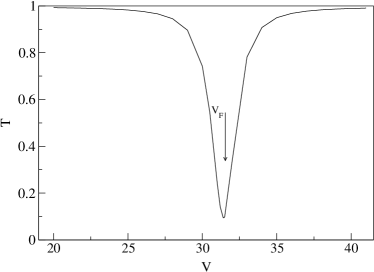
Figure 4: The transmission coefficient for the scattering of the soliton on the Fano defect, defined as in Eq. (21) and found from direct simulations, versus the soliton’s velocity $V$. Parameters are the same as in Fig. 3. The minimum is located at $V_{F}=2Cq_{F}$.

There is a minimum in the dependence of the transmission on soliton velocity exactly at $V_{F}=2Cq_{F}$, as it is predicted by Eq. (14) and the concept proposed above, according to which the soliton may be treated as a spectrally narrow packet of quasi-linear waves, hence the resonant backscattering should take place when the central wavenumber $q_{c}$ coincides with the linearly predicted Fano-resonance wavenumber, $q_{F}$. The minimum does not reach zero, which is explained by the finite spectral width $\Delta q_{c}$ of the soliton, i.e., wave components which build up the soliton do not fully backscatter. It should be stressed that the close proximity of the numerically found minimum to the anticipated point predicates upon the conditions (22) and (19), but it is not related to the fact that the particular example displayed in Fig. 4 has $q_{F}=\pi/2$. In fact, numerical results are very similar at other values of $q_{F}$.

To study the case when the wave-wave interactions are important during the time of the interaction between the soliton and the defect, i.e., $\tau_{\mathrm{int}}\,{}_{\sim}^{>}\,\tau_{\mathrm{disp}}$, the dispersion time was changed by shifting the soliton’s central wavenumber $q_{c}$ to the spectrum’s edge, keeping all other parameters fixed. The Fano resonance is observed in the simulations until $\tau_{\mathrm{int}}\approx\tau_{\mathrm{disp}}$. With the further decrease of $\tau_{\mathrm{int}}$, the Fano minimum in the $T(V)$ curve becomes less pronounced, and disappears at some critical value of $q_{c}$. For instance, we have found numerically that for $C=\eta=\lambda=\epsilon=1$, when the condition of the smallness of $\tau_{\mathrm{disp}}$ is fulfilled, the Fano resonance disappears at $q_{c}\approx 1.0$.

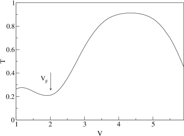
Figure 5: The dependence of the soliton’s transmission coefficient in the case of the scattering on the Fano defect on its velocity $V$. The parameters are $C=\eta=\lambda=\epsilon=1.0$, and $q=1$. The minimum at $V_{F}=2Cq_{F}$ is quite shallow in this case.

Still we observe a smooth $T(V)$ curve (Fig. 5). This result implies that the plane-wave modes which make up the soliton loose their resonant backscattering features. This is not unexpected, as the interaction of many modes between themselves can be interpreted as a multichannel scattering problem (as opposed to many uncoupled single-channel scattering processes in the absence of the mode-mode interaction). Multichannel scattering problems are expected to have less pronounced Fano resonance features, since the Fano resonance is inherently based on keeping phase coherence in order to support the destructive interference. As the phase coherence gets suppressed by the mode-mode interactions, the necessary interference is detuned.

III.2 Resonant transmission of solitons

The passage of a soliton through a single-site impurity has been already studied in many works oneimp . Here we consider the nonlinear extension of the two-site-impurity system (1),

$$i\dot{\phi}_{n}=C(\phi_{n-1}+\phi_{n+1})+\lambda|\phi_{n}|^{2}\phi_{n}+(\delta_{n,0}+\delta_{n,1})\epsilon\phi_{n}\;.$$ (23)

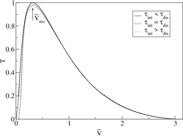
Figure 6: A typical dependence of the transmission coefficient $T$ for the soliton in the model (23) on $V$ for $\eta=\lambda=1.$ and (a) $\epsilon=19$ and $C=10$ (solid line); (b) $\epsilon=3.8$ and $C=2$ (dashed line); (c) $\epsilon=2.85$ and $C=1.5$ (dotted line) In this figure the normalized velocity $\bar{V}=\frac{V}{2C}$ is used. In all the cases, the position of the resonance is fixed at $\bar{V}_{res}\approx 0.318$.

The transmission coefficient for the soliton passing this defect was computed numerically for various values of parameters, and found to be in a very good agreement with Eq. (3), see Fig.6. Remarkably, neither the position of the resonance nor the value of the transmission coefficient at the resonance is conspicuously affected when the wave-wave interactions become important. This clearly indicates that dephasing does not seriously harm the resonant-transmission mechanism.

IV Conclusions

We have shown that solitons may be resonantly transmitted or backscattered depending on their velocity and the type of the scatterer. We explained these effects by considering the soliton as a superposition of plane-wave modes in the limit when the mode-mode interaction is not affecting the scattering process. By tuning parameters into a regime where the mode-mode interaction becomes essential during the scattering process, we have observed that the phase-insensitive resonant transmission is not affected. However, the Fano-resonant backscattering, which relies on the phase coherence in the two-channel scattering process, is completely suppressed in this case, which is a consequence of the dephasing of individual modes due to the interaction between them.

References

- (1) P. Sheng, B. White, Z. Zhang, and G. Papanicolaou, Scattering and localization of classical waves in random media, World Scientific, Singapore, (1989).
- (2) V. I. Klyatskin, and A. I. Saichev, Sov. Phys. Usp. 35, 231 (1992) [Usp. Fiz. Nauk 162, 161 (1992)].
- (3) I. M. Lifshitz, S. A. Gredeskul, and L. A. Pastur, Introduction to the theory of disordered systems, Wiley, New York (1988).
- (4) W. Zwerger, Theory of coherent transport in: Quantum transport and dissipation, Wiley, New York (1988).
- (5) D. Hennig, and G. P. Tsironis, Phys. Rep. 307, 333 (1999).
- (6) L. D. Landau and E. M. Lifshitz, Quantum Mechanics: non-relativistic theory, Oxford, Pergamon Press, 1977 .
- (7) C. Cohen-Tannoudji, B. Diu, and F. Laloe, Quantum mechanics, Paris, Hermann, 1977.
- (8) U. Fano, Phys. Rev. 124, 1866 (1961); J.A. Simpson and U. Fano, Phys. Rev. Lett. 11, 158 (1963).
- (9) G. D. Mahan, Many-particle physics, New York, Plenum Press (1993).
- (10) S.A. Gurvitz and Y.B. Levinson, Phys. Rev. B 47, 10578 (1993).
- (11) J.U. Nöckel and A.D. Stone, Phys. Rev. B50, 17415 (1994).
- (12) A. J. Sievers and J. B. Page: in Dynamical Properties of Solids VII Phonon Physics The Cutting Edge, ed. G. K. Horton and A. A. Maradudin (Elsevier, Amsterdam, 1995); S. Aubry, Physica D 103, 201 (1997); S. Flach and C. R. Willis, Phys. Rep. 295, 182 (1998).
- (13) S. Flach, A. E. Miroshnichenko and M. V. Fistul, Chaos, in press, cond-mat/0209427.
- (14) S. Flach, A. E. Miroshnichenko, V. Fleurov, and M. V. Fistul, Phys. Rev. Lett. 90, 084101 (2003).
- (15) S. Kim, C. Baesens, and R. S. MacKay, Phys. Rev. E 56, R4955 (1997); S. W. Kim and S. Kim, Physica D 141, 91 (2000); T. Cretegny, S. Aubry, and S. Flach, Physica D 199, 73 (1998).
- (16) H. S. Eisenberg, Y. Silberberg, R. Morandotti, A. R. Boyd, and J. S. Aitchison, Phys. Rev. Lett. 81, 3383 (1998).
- (17) J. W. Fleischer, T. Carmon, M. Segev, N. K. Efremidis, and D. N. Christodoulides, Phys. Rev. Lett. 90, 023902 (2003).
- (18) P. Tong, B. Li, and B. Hu, Phys. Rev. B 59, 8639 (1999).
- (19) B. A. Malomed and M. Ya. Azbel, Phys. Rev. B 47, 10402 (1993).
- (20) Y. S. Kivshar and B. A. Malomed, Rev. Mod. Phys. 61, 763 (1989).
- (21) X. D. Cao and B. A. Malomed, Phys. Lett. A 206, 177 (1995); T. Iizuka, H. Amie, T. Hasegawa and C. Matsuoka, Phys. Lett. A 220, 97 (1996); J. Cuevas, F. Palmero, J. F. Archilla and F. R. Romero, J. Phys. A: Math. Gen. 35, 10519 (2002).