Non-Life Insurance Pricing : Statistical Mechanics Viewpoint

Abstract

We consider the insurance company as a physical system which is immersed in its environment (the financial market). The insurer company interacts with the market by exchanging the money through the payments for loss claims and receiving the premium. Here in the equilibrium state we obtain the premium by using the canonical ensemble theory, and compare it with the Esscher principle, the well known formula in actuary for premium calculation. We simulate the case of car insurance for quantitative comparison.

I Introduction

From the first of nineteen century the economists have tried to find a way to use the formalism of physical theories in mathematical modeling of economy. The concepts of utility function and economical equilibrium entered into the financial theories in correspondence with potential energy and mechanical stability bjn . The physicists have paid less attention to this subject till last decade bjn . Recently they have more regards for studying the dynamics of the stock marketsbp ; ms . The main source of their interest comes from fluctuation of stock prices with the time. Understanding this behavior enable us to manage the strategies for trading sz . The statistical mechanics has appeared as a powerful method for exploring the price dynamics bjn ; bp ; ms ; sz .

The insurance is one of the important parts of the financial market with respect to trading risks. In the specified period of time, the results of a loss events (risks) that occur for the insurant are covered by insurance company and insurant also pays an amount of money to the insurer, which is called premium gv ; kpw . In the competitive financial market the calculation of premium is very complicated. The premium is affected by random nature of risks and also variation in number of the insurants. The latter may be decreased due to an increment in premium and is increased by reduction of premium. The actuary is a branch of mathematics that studies the relation between paid and received money in order to assign premium to a category of risks.

Nowadays the physicists also pay attention to this part of the financial market. They look for a new way for the premium calculation on the basis of physical concepts fd ; d .

In this paper we are intended to explain how the equilibrium statistical mechanics may be used for premium forecasting. In the next section we describe the analogy between the financial market and physical system in contact to heat reservoir. A method for equilibrium insurance pricing will be suggested based on the canonical ensemble theory. In the last section the special case of car insurance is simulated and we compare our method with Esscher principle which is the famous method in actuary gv and asset pricing gs ; b2 ; b3 ; vgdkd .

II Description of the Model

The financial market is combination of large number of economic agents which are interacting with each other through buying and selling. We consider the behavior of one of the agents for example an insurance company; all other agents may be regarded as its environment. The agent exchanges money when interacts with its environment. We suppose the financial market is a closed system, the environment will absorb the money that the agent loses and supplies the agent’s incomes. In equilibrium state a parameter that we denote it by $\beta$ has the same value for the agent and its environment p .

$$\beta_{Agent}=\beta_{Environment}$$ (1)

This parameter should be related to macroscopic properties of an economic agent. Later on, we signify it for an insurance company in terms of its initial wealth, the mean claim size and the ruin probability.

Like a physical system in contact with a heat reservoir we can nominate the following probability for $E(t)$, the net money which is exchanged between an agent and its environment at the end of specified time interval p ,

$$Pr(E(t))=\frac{e^{-\beta E(t)}}{\sum e^{-\beta E(t)}}$$ (2)

The sum is over all possible amounts of exchanged money in equilibrium state. We assume here that the agent’s money is considerably lesser than the money in the environment.

The above result is confirmed by simulation cc ; dy1 and is also inferred from empirical data dy2 ; dy3 .

For the special case of car insurance in the time interval $t$, the insurance company receives premium from $I(t)$ insurants and covers the loss results for $N(t)$ car accidents. In each accident insurant charges the company for $X_{j}$ amount of money. Thus the exchanged money at the end of interval is,

$$E(t)=pI(t)-\sum^{N(t)}_{j=1}X_{j}$$ (3)

Where $p$ is the premium. In the insurance terminology we call this money the surplus of company. The $I(t)$, $N(t)$ and $X_{j}$ are random variables which their probability distribution should be inferred from empirical data of the insurance company.

Premium calculation principle is a rule that assign to any distribution function (correspond with loss events) a real number gv . Bühlmann in his brilliant papers on economic premium principle stated that premium calculation principle should also depend on market conditions in addition to loss distribution b4 ; b5 . He constructed a model for whole insurance market with many agents; like insurance companies, reinsurance companies and buyers of insurance. He concluded that the sum of all incurred losses for all agents in the market shows the effect of surrounding market and it should be included in premium calculation principle.

In this work we introduce a new way for premium calculation. The number of insurants enters in our model as a reminiscence of the market conditions, the competition in the market changes it randomly as we mentioned above.

The insurance company avoids of financial failure. Premium should be calculated so that the surplus of company at the end of specified interval should be zero at least. This condition may be satisfied in mean.

$$<E(t)>=\sum Pr(E(t))E(t)=0.$$ (4)

In real case premium is greater than the value obtained from eq. 4 because administration expenditures must be compensated and company also likes to profit, anyhow we aren’t considering these matters.

If the number of insurants becomes constant then by simple calculation eq. 4 reduces to what is known as the Esscher principle.

$$pI_{0}=\frac{\sum Z(t)e^{\beta Z(t)}}{\sum e^{\beta Z(t)}}.$$ (5)

Where $Z(t)$ is the aggregate loss in the time interval $t$, it is defined as,

$$Z(t)=\sum_{j=1}^{N(t)}X_{j}$$ (6)

Unlike to the net premium that is obtained by averaging the aggregate loss, in the Esscher principle the premium is calculated by exponential tilting of loss events. The parameter $\beta$ appears to scale the weight of each event. There is no unique way for computing the $\beta$ parameter in Esscher principle; some authors use the optimization procedure gv and others relate it to the risk tolerance of the insurance company b4 . The way that we adopt in this paper for determination of this parameter is also applicable here.

The Esscher principle as an efficient method for premium computing appears as a special case of our method. The difference between it and our method is shown in the next section numerically.

III Simulation Results

To simulate our model, it is necessary to specify the distributions for the random quantities which are appeared in expression for the surplus, eq. 2.

By assumption the number of loss claims by insurants, $N(t)$ has Poisson distribution with the mean $\lambda t$. It depends only on the length of interval $t$ and also is statistically independent of the number of claims in any previous interval.

$$Pr(N(t+s)-N(s)=n)=\frac{{(\lambda t)}^{n}e^{-\lambda t}}{n!}$$ (7)

The important property of Poisson distribution is that the times between successive claims are independent and identically exponentially distributed (the Erlang’s model) with the mean $1/\lambda$. It is what we encounter in most of the real cases.

The model for the claim size is constructed based on the knowledge and experience of the insurance company in addition to data from the past. The model should provide a balance between simplicity and conformity to the available data.

The purpose of this paper is explanation of our method; in this respect for simplicity we restrict ourselves to the exponential distribution for the claim size. Otherwise we are forced to do a lengthy numerical computation that don’t correspond to our goal.

$$Pr(X=\xi)=\frac{1}{\mu}e^{-\xi/\mu}$$ (8)

The $\mu$ is the mean of the claim size. The product of the $\lambda t$ and $\mu$ is the net premium, $p_{0}$. The insurance company which offer this value or less for the premium will be busted ultimately kpw .

The distribution for the number of insurants has not been modeled since now because it doesn’t be involved in the traditional methods for calculating the premium. The eq. 4 shows its importance in our method. However we assume the number of insurants is distributed uniformly with the mean, $I_{0}$, and standard deviation, $\%10I_{0}$. This assumption based on empirical data of the Iran Insurance Company r .

All the necessary parameters for tuning the mentioned distribution functions are obtained from statistical reports of Iran Insurance Company for the case of car insurance in year 2000 r . For independence of the results to any monetary units, the initial wealth and premium are expressed in terms of the mean claim size and net premium. The following results are averaged over 10000 different possible states of the modeled insurance company.

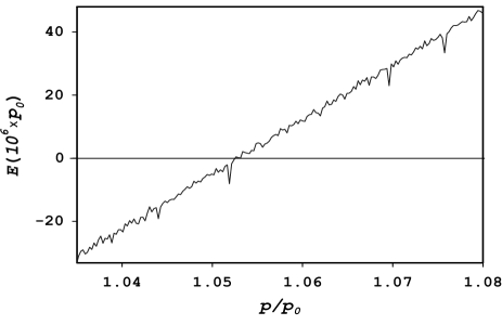
Figure 1: The annual profit or surplus after $300$ days versus the premium for large $\beta$. The premium and surplus are measured in terms of net premium.

The variation of annual profit or surplus after $300$ days with premium for large $\beta$, is shown in the fig. 1. The desired value for the premium is obtained from calculation of the intersection point of approximated curve with the premium axis. For other values of the parameter $\beta$ we can apply the same method for computing the premium.

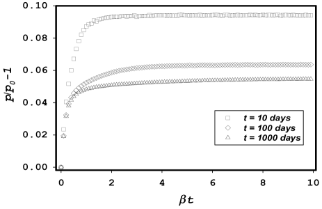
Figure 2: The premium as a function of $\beta t$. The results for $t=10,100$ and $1000$ is plotted.

The premium is also function of parameter $\beta$. In the case of $\beta=0$ it is equal to the net premium. An increment in $\beta$ increases the premium but for large $\beta$ it approaches to a limiting value. The fig. 2 shows this behavior for three value of the time interval.

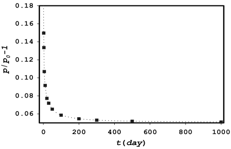
Figure 3: The premium versus duration of the insurance contract for the large $\beta$. The squares are obtained by simulation and the curve shows the fitting result.

The fig. 3 demonstrates dependency of the premium on duration of insurance contract for the large $\beta$. This behavior is expected in the insurance market kpw . The premium for other values of the parameter $\beta$ shows the same behavior in the time.

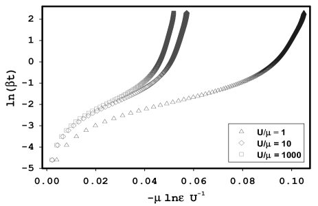
Figure 4: The parameter $\ln(\beta t)$ as a function of $\mu ln\varepsilon U^{-1}$ which is introduced in the text. The results for $U=1,10$ and $1000$ times of the mean claim size are plotted.

The parameter $\beta$ has been ambiguous since now. At this moment we proceed to clear its meaning. It can be understood by dimensional analysis of the eqs. 3 and  4 that the parameter $\beta$ is proportional to the inverse of time. The fig. 2 also confirms this statement, the behavior of the premium as a function of $\beta t$ is the same for different time intervals in exception of their limiting values.

The most important quantities which are used by the insurers for their financial decisions are the initial wealth $U$ and the ultimate ruin probability $\varepsilon$. The combination of them with the mean claim size $\mu$ is used in all methods for calculating the premium gv ; kpw . The parameter $\beta$ is also function of these quantities. The fig 4 shows the $\ln\beta t$ as a function of the dimensionless parameter $-\mu\ln\varepsilon U^{-1}$ and the initial wealth. This consequence is issued from relation of the ultimate ruin probability on premium kpw ,

$$\varepsilon={p_{0}\over p}\exp{[-{U\over\mu}({p_{0}\over p}-1)]}.$$ (9)

And the result for dependency of premium on $\beta t$ which is also shown in fig. 2.

The ultimate ruin probability for exponential distribution of claim size can be calculated analytically as is seen in the eq. 9, but in other cases it would be computed numerically from the following relation kpw ,

$$\varepsilon=1-\sum_{k=0}^{\infty}(1-{p_{0}\over p})({p_{0}\over p})^{k}F_{e}^{*k}(U).$$ (10)

Where $F_{e}(x)$ is related to the claim size probability $F(x)$,

$$F_{e}(x)={1\over\mu}\int_{0}^{x}[1-F(y)]dy$$ (11)

And $F_{e}^{*k}(U)$ is the $k$-fold convolution of $F_{e}(U)$ with itself.

The fig. 4 also indicates if the initial wealth becomes large for a fixed time interval the parameter $\beta$ approaches to zero. This means that a wealthy company buys the risks with the less premium in comparison to the small companies which offer more expensive insurance. This fact conforms to our experience in the financial market.

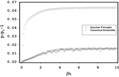
Figure 5: The premium versus the parameter $\beta t$ for $100$ days interval. The results of our method (canonical ensemble theory) and Esscher principle are plotted for comparison.

As mentioned before the Esscher principle is concluded from our method. The variation in number of insurants changes the premium certainly. The fig. 5 displays the difference between two methods numerically.

IV summary

We construct a simple model for the cash flow in an insurance company for the category of non-life insurance. A new method is suggested for calculation of premium on the basis of the canonical ensemble theory. This method considers the effect of the environment (or market conditions) by introducing a new random variable, the number of insurants, into the equation of cash flow. In this respect the empirical data of an insurance company is sufficient for take into consideration of environment conditions. There is no need to acquire any information about other agents in the market unlike the Bühlmann method. Another advantage of this method is ability for extension in the small market case. The latter is under investigation by the author.

The financial backbone of insurer company is concealed in the parameter $\beta$ which play essential role in our method for computing the premium. When we omit the effect of market conditions by considering constant value for number of insurants the Esscher principle is emerged as a result. Difference between our method and the Esscher principle that is apparently due to the effects of environment is shown numerically.

This work has been supported by the Zanjan university research program on Non-Life Insurance Pricing No 8243.

References

- (1) Z. Burda, J. Jurkiewicz and M. A. Nowak, Is Econophysics a Solid Science?, Acta Physica Polonica B, 34, 87 (2003).
- (2) J.P. Bouchaud and M. Potters, Theory of Financial Risks, Cambridge University Press, Cambridge, (2000).
- (3) R. Mantegna and H.E. Stanely, An Introduction to Econophysics, Cambridge University Press, Cambridge, (2000).
- (4) D. Sornette and W. X. Zhou, The US 2000-2002 market descent, Quant. Finance, 2, 468 (2002).
- (5) M. J. Goovaerts and F. deVylder, Insurance Premium, North Holland, Amsterdom, (1984).
- (6) S. A. Klugman, H. H. Panjer and G. E. Willmot, Loss Models: From Data to Decisions, John Wiley, New York, (1998).
- (7) M. E. Fouladvand and A. H. Darooneh, Premium Forecasting for an Insurance Company, Second Nikkei Workshop and Symposium on Econophysics (Ed. H. Takayasu), 313 , Springer, Berlin, (2003).
- (8) A. H. Darooneh, Non Life Insurance Pricing, Proceeding of 18-th Annual Iranian Phys. Conf., 162 (2003). in persian
- (9) H. U. Gerber and Shiu E. S. W., Option Pricing by Esscher Transforms, Transaction of the Society of Actuaries,XLVI, 99 (1994).
- (10) H. Buhlmann, F. Delbaen, P. Embrechts and A. Shirayev, No-Arbitrage Change of Measure and Conditional Esscher Transform, CWI Quarterly,9, 291 (1997).
- (11) H. Buhlmann, F. Delbaen, P. Embrechts and A. Shirayev, On Esscher Transform in Descrete finance Model, ASTIN Bulletin,28, 171 (1998).
- (12) D. Vyncke, M. J. Goovaerts, A. DeSchepper, R. Kass and J. Dhaene, On the Distribution of Cash-Flows using Esscher Transforms, Journal of Risk Insurance,70, 563 (2003).
- (13) R. K. Pathria, Statistical Mechanics, Pergamon Press, Oxford, (1972).
- (14) A. Chatterjee and B. K. Chakarbarti, Money in Gas-Like Market, Physica Scripta, T90, 36 (2003).
- (15) A. Drgulescu and V. M. Yakovenko, Statistical Mechanics of Money, Eur. Phys. J. B, 17, 723 (2000).
- (16) A. Drgulescu and V. M. Yakovenko, Evidence for the Exponential Distribution of Incomes in the USA , Eur. Phys. J. B, 20, 585 (2001).
- (17) A. Drgulescu and V. M. Yakovenko, EExponential and Powe Law Probability Distribution of Wealth and Incomes in the United Kingdom and United States , Physica A, 299, 213 (2001).
- (18) H. Buhlmann, An Economic premium Principle, ASTIN Bulletin,11, 52 (1980).
- (19) H. Buhlmann, General Economic premium Principle, ASTIN Bulletin,14, 13 (1984).
- (20) —– , Statistical Report of Iranian Insurance Industry, Iran Central Insurance Company, Tehran, (2000).