Dynamics of magnetic flux lines in the
presence of correlated disorder

Abstract

We investigate the dynamics of interacting magnetic flux lines driven by an external current in the presence of linear pinning centers, arranged either in a periodic square lattice or placed randomly in space, by means of three-dimensional Monte Carlo simulations. Compared to the non-interacting case, the repulsive forces between the vortices reduce the critical current $J_{c}$, as determined from the depinning threshold in the current-voltage (I-V) characteristics. Near the depinning current $J_{c}$, the voltage power spectrum $S(\omega)$ reveals broad-band noise, characterized by a $1/\omega^{\alpha}$ power law decay with $\alpha\leq 2$. At larger currents the flux lines move with an average velocity $v_{cm}$. For a periodic arrangement of columnar pins with a lattice constant $d$ and just above $J_{c}$, distinct peaks appear in the voltage noise spectrum $S(\omega)$ at $\omega\sim v_{cm}/d$ which we interpret as the signature of stick-slip flux line motion.

1 Introduction

Magnetic vortices in the mixed state of high-$T_{c}$ superconductors in the presence of defects — either localized point pinning centers, such as oxygen vacancies or extended columnar pins introduced into the material via high-energy ion irradiation — offer a complex system which has attracted the attention of both experimentalist and theorists from various disciplines of physics in recent years [1]. This area of research is also inspired by important technological questions triggered by the search for effective pinning centers in order to minimize dissipation when current is passed through the superconductor [1]. From a more fundamental viewpoint, one is interested in the non-equilibrium dynamics of a disordered flux line system. When subject to an external electric current, non-trivial steady states are generated which can be directly probed experimentally. For example, the current-voltage (I-V) characteristics [1], the voltage noise power spectrum [2, 3, 4], or the local flux density noise [3] measured in experiments bear important signatures of the different non-equilibrium steady states. At low currents, transport can take place due to thermally activated ‘tunneling’ of flux lines through the defects [1], while at larger currents various intriguing steady states have been proposed, such as plastic flow where flux lines move in channels [5]. With increasing current the flux lines tend to reorder and move in a lattice (moving Bragg glass for point vortices [6, 7]), or the channels in the plastic flow regime can organize in a periodic structure (smectic phase) in the transverse direction of the external current [7].

The presence of such steady states is reflected in the voltage noise spectrum; e.g., reordering would give rise to characteristic ‘washboard’ noise features. Recent experiments have in fact demonstrated the presence of both narrow- and broad-band noise in the measured voltage and local flux density spectra [2, 3, 4]. Our goal is in addition to study how these noise spectra depend on the type of defects (correlated or point-like) present in the sample. However, since analytical studies of the vortex dynamics are usually limited to asymptotic regimes [1, 8, 9] where the current $J$ is either much smaller or much larger than the critical current $J_{c}$, one needs to resort to either Langevin molecular dynamics simulations [5, 10, 11, 12] or Monte Carlo techniques [13, 14] to study the various non-equibrium steady states which occur in the intermediate current regime. Owing to their complexity, these numerical simulations are largely restricted to two dimensions [5, 10, 11, 12] and very few three-dimensional studies have been reported [13, 14, 15, 16, 17]. In this article we present the results of fully three-dimensional Monte Carlo simulations of interacting magnetic vortex lines in the presence of columnar defects. We investigate the effects of the repulsive forces between the flux lines and their interactions with extended defects in the I-V characteristics and the voltage noise spectrum, focusing on those aspects which are inaccessible by two-dimensional simulations.

This article is organized as follows. The model is introduced in Sec. II and the Monte Carlo scheme is described in Sec. III. In Sec IV we present the results of our simulations for the I-V characteristics and voltage noise power spectra. Some conclusions are offered in Sec. V.

2 The model

We consider a system consisting of $n$ flux lines in the London approximation in the presence of $N_{p}$ defects. Our description utilizes an effective Hamiltonian [6]

$$H[{\bf r}_{i}]=\sum_{i=1}^{n}\frac{\varepsilon}{2}\int_{0}^{L}ds\left[\frac{1}{\Gamma^{2}}\left(\frac{d{\bf r}_{i\perp}(s}{ds}\right)^{2}+\left(\frac{dz_{i}(s)}{ds}\right)^{2}\right]$$ (1)

$$+\sum_{i,j=1;i\neq j}^{n}\epsilon_{int}\int_{0}^{L}ds\,K_{0}\!\bigg{(}\frac{|{\bf r}_{i\perp}(s)-{\bf r}_{j\perp}(s)|}{\lambda_{ab}}\bigg{)}+\sum_{i=1}^{n}\int_{0}^{L}ds\,V_{p}[{\bf r}_{i}(s)]\ ,$$

where ${\bf r}_{i}(s)\equiv[{\bf r}_{i\perp}(s),z_{i}(s)]$ describes the configuration of the $i$th flux line in three dimensions, and the crystalline axis ${\bf c}$ of the superconducting material (as well as the external magnetic field) is oriented parallel to $\hat{\bf z}$, in a sample of thickness $L$. The first term gives the line tension energy of a magnetic flux line. This linear elastic form of energy holds good as long as $|d{\bf r}_{\perp}(z)/dz|<1/\Gamma$ [18], where $\Gamma$ denotes the anisotropy ratio [1, 8]. The line stiffness is given by $\varepsilon\approx\varepsilon_{0}\ln(\lambda_{ab}/\xi_{ab})$ [1, 8], with $\varepsilon_{0}=(\phi_{0}/4\pi\lambda_{ab})^{2}$ ($\phi_{0}=hc/2e$ is the magnetic flux quantum). $\lambda_{ab}$ and $\xi_{ab}$ denote the penetration depth and the superconducting coherence length in the $ab$ plane, respectively. For high-$T_{c}$ materials, $\Gamma\gg 1$ [1], giving the quadratic form of the line tension energy a wider range of validity. The repulsive interaction energy between the flux lines is approximated to be local in the $z$ coordinate, in accord with the London limit. It is represented by the second term in (1), where $\epsilon_{int}=\phi_{0}^{2}/(8\pi^{2}\lambda_{ab}^{2})$ and $K_{0}(x)$ is the modified Bessel function which varies as $-\ln x$ when $x\ll 1$ and $\sim x^{-1/2}e^{-x}$ as $x\gg 1$. We model the pinning potential as a sum of $N_{p}$ independent potential wells, $V_{p}[{\bf r}(s)]=\sum_{k=1}^{N_{p}}U\Theta(r_{p}-|{\bf r}(s)-{\bf r}^{(p)}_{k}|)$, where $r_{p}$ is the radius, $\Theta(x)$ denotes the Heaviside step function, and the ${\bf r}^{(p)}_{k}$ indicate the $N_{p}$ locations of the pinning sites. The free energy $F_{L}(T)$ per unit length is then defined through $\exp[-\beta F_{L}(T)L]=\int\prod_{i=1}^{n}D[{\bf r}_{i}]\exp\left(-\beta H[{\bf r}_{i}]\right)$, where $\beta=(k_{B}T)^{-1}$. We study the dynamics of the flux lines when an external current ${\bf J}$ is applied through the system which produces a Lorentz force ${\bf f}_{L}=(1/c)\hat{z}\times{\bf J}=(J/c)\,\hat{\bf x}$, per unit length of each flux line. We resort to a three-dimensional Monte Carlo (MC) simulation to deal with the system in an intermediate range of driving currents where the system appears to be intractable by means of analytical methods.

3 Monte Carlo simulation

In our Monte Carlo simulation each flux line ${\bf r}(s)$ is modeled by $N=L/a_{0}$ points where the $i$th point is located at ${\bf r}(i)\equiv[x(i),y(i),z(i)]$ and interacts with its nearest neighbors via a simple harmonic potential $\frac{\varepsilon}{2}\sum_{\langle j\rangle=i-1,\,i+1}\,[\Gamma^{-2}({\bf r}_{\perp}(i)-{\bf r}_{\perp}(\langle j\rangle))^{2}+(|z(i)-z(\langle j\rangle)|-a_{0})^{2}]$. The line is placed in a box of size $L_{x}\times L_{y}\times L_{z}$ with periodic boundary conditions in all directions. The interaction energy between a pair $(l,m)$ of flux lines is given by $\epsilon_{int}\sum_{i=1}^{N}K_{0}(|{\bf r}_{\perp l}(i)-{\bf r}_{\perp m}(i)|/\lambda_{ab})$. To calculate the interaction energy we resort to a well-known method [19] of truncating the potential beyond a cut-off length $l_{cutoff}\gg\lambda_{ab}$ in order to keep the computation time within a sensible limit. We make sure that our results do not depend on the size of $l_{cutoff}$. Since we are interested in studying the effects of defect correlations in the dynamics, we restrict our simulation to low temperatures $T/T^{*}<1$. Here $T^{*}$ denotes the temperature where entropic corrections due to thermal fluctuations become relevant for pinned flux lines [6]. The columnar pins and point defects are respectively modeled by uniform cylindrical or spherical potential wells of (uniform) strength $U$ and radius $b_{0}$. The cylindrical wells are oriented parallel to the c axis. We investigate the dynamics for three different distributions of defects, namely, (i) columnar pins either distributed randomly, or (ii) arranged in a square lattice in the $xy$ plane, and (iii) point defects distributed randomly in the sample. Since in the presence of weak currents ${\bf J}=-J\hat{\bf y}$ the flux lines locally move according to equilibrium dynamics, one may incorporate the effect of the force in the MC by introducing an additional work term $-\sum_{i=1}^{n}{\bf f}_{L}\cdot\int_{0}^{L}ds\,{\bf r}_{i}(s)$ in the Hamiltonian (1) [8, 13, 14].

To initiate the simulation, flux lines of straight configurations parallel to the ${\hat{\bf z}}$ axis are nucleated at random positions in the $xy$ plane. We then let the system equilibrate. Once equilibrium has been reached we turn on the external current and let the system evolve. We have checked that the results in the steady state are independent of the initial configurations. At each trial a randomly chosen point on the line is updated according to a Metropolis algorithm [20]. The point can then move in a random direction a maximum distance of $\triangle<b_{0}/\sqrt{3}$ to guarantee interaction with every defect. In the simulation the values $z_{i}$ are held fixed; we have checked that our results do not change qualitatively even if these positions $z_{i}$ are allowed to fluctuate [16].

The drift velocity of the flux lines is proportional to the average velocity of the center of mass (CM) ${\bf v}_{cm}=n^{-1}\sum_{i=1}^{n}\langle\overline{[{\bf R}_{i\,cm}(\tau)-{\bf R}_{i\,cm}(0)]/\tau}\rangle$, where ${\bf R}_{i\,cm}(\tau)-{\bf R}_{i\,cm}(0)$ is the distance traversed by the CM of the $i$th flux line in a time interval of length $\tau$; $\langle\cdot\cdot\cdot\rangle$ and the overbar denote the averages over Monte Carlo steps (MCS) in the steady state and over different disorder realizations, respectively. The voltage drop measured in experiments is caused by the induced electric field ${\bf E}={\bf B}\times{\bf v}_{cm}/c$ [21]. All length and energy scales are measured in units of $b_{0}$ and $\varepsilon_{0}$, respectively. The average distance between the defects for a uniform random distribution and the lattice constant for the periodic array of columnar pins was taken as $d=15\,b_{0}$. The parameters $\lambda_{ab}$, $\xi_{ab}$, $\varepsilon$, $U$, and $\Gamma$ were chosen to be $56\,b_{0}$, $0.64\,b_{0}$, $4\,\varepsilon_{0}$, $0.0075\,\varepsilon_{0}$, and $4$ respectively in the simulation; these numbers are consistent with the experimental data for high-$T_{c}$ materials [1]. Therefore thermally induced bending and wandering of the flux lines are largely suppressed, and we can interpret our results in terms of low-temperature dynamics. In the simulations all sets of data were collected in the steady state, which was typically reached after $t>10^{5}$ MCS and $t>10^{6}$ MCS for columnar defects and point pins, respectively. The size of the system ranged from $60\times 9\times 60$ to $2000\times 9\times 60$ in the simulations, and the data were averaged over $20$ to $50$ realizations of disorder. The value of $\tau$ ranged from $30$ to $500$ MCS in the simulations.

4 Results

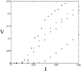
Figure 1: I-V characteristics for interacting flux lines in the presence of columnar defects with random ($\times$) and periodic ($\circ$) spatial distribution. Note that $J_{c}$ is almost the same in both situations. The corresponding I-V plot for a single flux line with periodically arranged columnar defects ($\triangle$) shows a higher $J_{c}$ (see text). In the non-interacting (single line) case with columnar pins $J_{c}$ is almost two times larger as compared to the interacting system. The I-V plot for a single flux line with random point defect distribution ($\ast$) is also given for comparison (see text). For currents $J>J_{c}$ the system with randomly distributed columnar pins displays a larger resistance (higher average vortex velocity) than the one with a periodic defect distribution.

In the absence of disorder and any external drive, at low temperatures (in our simulations $T<T^{*}\ll T_{c}$) the flux lines arrange themselves in a triangular Abrikosov lattice [21]. In the presence of disorder the lattice structure is replaced by glass phases [6], namely the so-called vortex glass in the case of uncorrelated point disorder, and the Bose glass in the presence of columnar defects [1]. As an external current is applied the nearly localized vortices (since $T<T^{*}$ the flux lines rarely tunnel through the defects) in the glassy phases start moving once a critical driving current is reached. At $T=0$, and in the absence of mutual vortex interactions, the flux lines are strictly bound to one or more pins in equilibrium. At the critical depinning current $J=J_{c}$ one then encounters a continuous non-equilibrium phase transition [22, 23, 24]. This zero-temperature phase transition becomes rounded to a crossover at $T>0$, but a characteristic ‘critical’ current separating the localized and moving vortex regimes can still be inferred at sufficiently low temperatures, as seen in the I-V characteristics displayed in Fig. 1, which were computed at $T=0.25\times 10^{-3}\varepsilon\ll T^{*}$.

It turns out that the critical current $J_{c}$ is actually higher for a system with columnar pins as compared to point disorder because of the increased defect correlations [16]. However the value of $J_{c}$ is the same for both random and periodic spatial distribution of the pins [16]. Repulsive interactions between the flux lines facilitate flux creep which is reflected in the delocalization of the vortices at a considerably lower current than for the non-interacting case (Fig. 1). The I-V characteristics also reveal that the voltage at the same current is higher for the system with a random as compared to periodic defect distribution. Similar behavior is observed in the dynamics of the single flux line, and can be qualitatively explained by an effectively faster transit time in the random pin distribution compared to the periodic columnar defect array [16]. We have also found that in the system with a single flux line in the presence of a periodic pin arrangement the I-V characteristics depends strongly on the orientation of J with respect to the lattice direction, for this determines the effective density of defects encountered by the moving vortex. A similar feature is likely to survive in the presence of interactions.

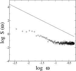
Figure 2: Log-log plot of the velocity noise power spectrum $S(\omega)$ vs. frequency $\omega$ for a system with columnar defects near the depinning threshold at $J\approx J_{c}$. The solid line, given as a guide, has slope $-2$.

The velocity (proportional to the induced voltage) noise is calculated by computing the velocity fluctuations about ${\bf v}_{cm}$. We evaluate the power spectrum $S(\omega)=\overline{\tilde{v}_{x}(\omega)\tilde{v}^{\ast}_{x}(\omega)}$, where $\tilde{v}_{x}(\omega)$ is the Fourier transform of the velocity fluctuation $\tilde{v}_{x}=n^{-1}\sum_{i=1}^{n}[v_{ix}-\langle v_{ix}\rangle]$, with $v_{ix}(t)=[X_{i\,cm}(t+\tau)-X_{i\,cm}(\tau)]/\tau$ being the center-of-mass velocity of the $i$th flux line.

Near $J_{c}$ we observe a power-law decay in the voltage noise spectrum: $S(\omega)\sim 1/\omega^{\alpha}$, where an effective exponent $\alpha\approx 2$ is observed for almost a frequency decade in the system with periodically arranged columnar pins (Fig. 2). At low frequencies there are indications that the effective exponent may be smaller than $2$. For a single line in the presence of random point defects and at $T=0$, the value of $\alpha$ can be determined through a functional renormalization group calculation which gives $\alpha=1.5$ to one-loop order in three dimensions [23, 24], with corresponding mean-field value $\alpha=2$. The power law behavior observed in the simulation (Fig. 2) can be interpreted as a remnant of the zero-temperature depinning transition. In experiments [4], such broad-band noise (BBN) features show a $\omega^{-\alpha}$ decay with $\alpha\approx 2$.

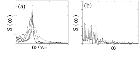
Figure 3: (a) Plot of the velocity noise power spectrum $S(\omega)$ vs. $\omega/v_{cm}$ for a system with columnar pins arranged in a periodic array for $J=0.05$ (circles), $J=0.07$ (squares), and $J=0.09$ (triangles). The peaks occur at the same scaled frequency $\tilde{\omega}\propto v_{cm}/d$. Note that the width of the peak decreases as $J$ is increased indicating the wider separation between the time scales $\tau_{r}$ and $\tau_{v}$. (b) Plot of $S(\omega)$ vs. $\omega$ for columnar pins distributed randomly in the sample for $J=0.05$ (squares). Notice the presence of secondary peaks in the spectrum (see text).

For currents $J>J_{c}$, three distinct time scales can appear in the dynamics: the residence time $\tau_{r}$ which is the duration a vortex line is trapped on the defects, $\tau_{v}$, the time taken by the flux line to travel between the pins, and $\tau_{w}$, the time taken by the moving vortex lattice in the event of reordering to traverse a distance of the lattice constant. In the regime where these time scales are well separated and $\tau_{r}<\tau_{v}$, as well as $\tau_{r}<\tau_{w}$, we can expect $\tau_{v}$ and $\tau_{w}$ to produce pronounced peaks in the velocity noise spectrum. We first summarize the results from the non-interacting case where the time scale $\tau_{w}$ is entirely absent (stick-slip motion). In Fig. 3(a) we plot $S(\omega)$ at different driving currents for a periodic distribution of columnar pins. The spectra reveal a single peak corresponding to the frequency $\tilde{\omega}\propto v_{cm}/d\propto 1/\tau_{v}$. Note that the width of the peak decreases as the external current ${\bf J}$ increases, which widens the time scale separation between $\tau_{r}$ and $\tau_{v}$. In a random defect distribution, see Fig. 3(b), there would be a distribution of the time scales $\tau_{v}$ around the average value $d/v_{cm}$. Therefore there could be many secondary peaks present in the spectrum arising due to the distribution of $\tau_{v}$ in addition to the principle peak which corresponds to $\tau_{r}\propto d/v_{cm}$. These secondary peaks would eventually diminish in intensity as the distribution of the time scales will narrow down at $d/v_{cm}$ with the results averaged over more defect configurations. Unlike for correlated defects, the time scales $\tau_{r}$ and $\tau_{v}$ are not well separated for point pins and the peaks turns out to be considerably suppressed as compared to the situation for columnar defects [16].

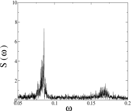
Figure 4: Plot of the velocity noise spectrum $S(\omega)$ vs. $\omega/v_{cm}$ for a system of periodically arranged columnar pins at $J=0.07$ with interacting flux lines. The primary peak corresponds to the rescaled frequency $\tilde{\omega}\propto v_{cm}/d$.

The presence of interactions between the flux lines may introduce the third time scale $\tau_{w}$ if the vortex lines align themselves into a lattice structure at large external currents. For example the predicted moving vortex lattice (in the presence of point defects) [7] would give rise to a distinct $\tau_{w}\propto a_{m}/v_{cm}$, where $a_{m}$ is the lattice constant of the moving flux line array. We have not yet detected any signature of the corresponding narrow-band noise in the presence of columnar defects with periodic spatial distribution, even when the average distance between the flux lines is much less than the periodicity of the pins. This implies absence of reordering in the observed range of external currents. We do find a peak in $S(\omega)$ corresponding to $\tau_{v}\propto d/v_{cm}$ (Fig. 4) which is also observed in the non-interacting case. However we might expect reordering when the density of the flux lines is larger than the defect density because then the effect of defect correlations becomes masked.

We have noticed a marked difference in $S(\omega)$ between columnar and point pins which results from the lack of spatial correlation in the $z$ direction for the point disorder. Notice that this distinction can be observed only in a three-dimensional dynamical simulation. It is due to a generic difference between correlated and localized pinning potentials. The ensuing absence or presence of the narrow-band noise peaks in the voltage noise spectrum $S(\omega)$, and its specific features, could perhaps be utilized as a signature to identify and characterize the type of disorder present and responsible for flux pinning in experimental superconducting samples as well.

5 Conclusion

In conclusion we have investigated the three-dimensional dynamics of interacting flux lines in the presence of correlated defects, either arranged in a periodic array or placed randomly in space. We find that the nature of the current-voltage characteristics depends on the defect correlation as well as the spatial distribution of the pinning centers. The voltage noise spectrum shows pronounced peaks in the case of correlated pins. The difference in the power spectra at $J>J_{c}$ between columnar and point disorder may serve as a novel diagnostic tool to characterize the pinning centers in superconducting samples.

6 Acknowledgements

We would like to thank S. Bhattacharya, A. Maeda, B. Schmittmann, and R. K. P. Zia for valuable discussions. This research has been supported by the National Science Foundation (grant no. DMR 0075725) and the Jeffress Memorial Trust (grant no. J-594). JD is supported by a Department of Energy grant through Lawrence Berkeley National Laboratory.

References

- [1] G. Blatter, M. V. Feigel’man, V. B. Geshkenbein, A. I. Larkin, and V. M. Vinokur, Rev. Mod. Phys. 66, 1125 (1994).
- [2] Y. Togawa, R. Abiru, K. Iwaya, H. Kitano, and A. Maeda, Phys. Rev. Lett. 85, 3716 (2000).
- [3] A. Maeda, T. Tsuboi, R. Abiru, Y. Togawa, H. Kitano, K. Iwaya, and T. Hanaguri, Phys. Rev. B 65, 054506 (2002).
- [4] A. C. Marley, M. J. Higgins, and S. Bhattacharya, Phys. Rev. Lett. 74, 3029 (1995).
- [5] C. J. Olson, C. Reichhardt, and F. Nori, Phys. Rev. Lett. 80, 2197 (1998); Phys. Rev. Lett. 81, 3757 (1998).
- [6] D. R. Nelson, Correlations and transport in vortex liquids, in: Defects and Geometry in Condensed Matter Physics, (Cambridge University Press, Cambridge, 2002), p. 271.
- [7] T. Nattermann and S. Scheidl, Adv. Phys. 49, 607 (2000).
- [8] D. R. Nelson and V. M. Vinokur, Phys. Rev. B 48, 13060 (1993).
- [9] D. R. Nelson, Vortex line fluctuations in superconductors from elementary quantum mechanics, in: Defects and Geometry in Condensed Matter Physics, (Cambridge University Press, Cambridge, 2002), p. 245.
- [10] M. Dong, M. C. Marchetti, A. A. Middleton, and V. M. Vinokur, Phys. Rev. Lett. 70, 662 (1993).
- [11] C. Tang, S. Feng, and L. Golubovic, Phys. Rev. Lett. 72 (1994) 1264.
- [12] C. Reichhardt and C. J. Olson, Phys. Rev. B 65, 0943011 (2002) .
- [13] S. Ryu, A. Kapitulnik, and S. Doniach, Phys. Rev. Lett. 71, 4245 (1993).
- [14] S. Ryu and D. Stroud, Phys. Rev. B 54, 1320 (1996).
- [15] A. Schönenberger, A. Larkin, E. Heeb, V. Geshkenbein, and G. Blatter, Phys. Rev. Lett. 77, 4636 (1996) .
- [16] J. Das, T. J. Bullard, and U. C. Täuber, Physica A 318, 48 (2003).
- [17] Qing-Hu Chen and Xiao Hi, Phys. Rev. Lett. 90, 117005 (2003).
- [18] E. H. Brandt, Phys. Rev. Lett. 69, 1105 (1992).
- [19] D. Frenkel and B. Smit, Understanding Molecular Simulation: From Algorithms to Applications, 1st ed. (Academic Press, NY, 1996).
- [20] M. E. J. Newman and G. Barkema, Monte Carlo methods in Statistical Physics (Clarendon Press, Oxford, 1989).
- [21] M. Tinkham, Introduction to Superconductivity (McGraw-Hill, NY, 1975).
- [22] O. Narayan and D. S. Fisher, Phys. Rev. B 48, 7030 (1993) .
- [23] D. Ertas and M. Kardar, Phys. Rev. Lett. 73, 1703 (1994) .
- [24] M. Kardar and D. Ertas, Non-equilibrium dynamics of fluctuating lines, in: Proceedings of the NATO Advanced Study Institute on Scale Invariance, Interfaces, and Non-Equilibrium Dynamics, eds. A. McKane, M. Droz, J. Vannimenus, and D. Wolf (Plenum, New York, 1995), p. 89.