High–$T_{c}$ RF SQUIDs
with Large Inductance of Quantization Loop

Abstract

Experimental data on signal and noise characteristics of high–$T_{c}$ RF SQUIDs with large inductance of quantization loop are presented. The SQUIDs were produced by a thick–film HTS–technique of painting on the Y₂BaCuO₅ substrate. For the first time, a steady quantum interference was observed in RF SQUID with the inductance as large as $L_{S}=6.6$ nH, that is, 60 times higher than the fluctuation inductance $L_{F}\simeq 10^{-10}H$ at the liquid nitrogen temperature $T=77$ K. A new method is offered to evaluate the sensitivity of RF SQUID with optimum inductance of the quantization loop.

Introduction

At the beginning of the 90th, at the Institute in Physical–Technical Problems, Dubna, an original way of preparation high–temperature superconducting (HTS) YBa₂Cu₃O_7-δ thick films (TFs) by a quasi binary technique Vuong_1993 , was developed. The superconducting layer of YBa₂Cu₃O_7-δ was formed during the reaction of synthesis between the chemically active Y₂BaCuO₅ substrate and the layer of “paint” prepared from a mixture of BaCuO₂ and CuO, which was applied to the substrate.
A modification of this technique by means of the melting–growing (MG) technology Murakami_1992 allowed one to obtain the TFs with microscopic inclusions of the Y₂BaCuO₅–phase, which play the role of additional pinning centers in the YBa₂Cu₃O_7-δ–matrix Vuong_1994 .
Temperature and field dependency study of the AC susceptibility of these MG TF structures shows that pinning force is increased several times as compared with TF reference samples (without MG) which superconductive characteristics are similar to those of the samples synthesized by the conventional ceramic technique Vuong_1994 . The high density (minimum porosity) is an important feature of the MG TFs, and determines higher stability of such structures against a degradation process. Next, one–hole RF SQUIDs (see Fig. 1) were built on the basis of the MG TFs with the help of a developed method of making SQUID bridges (by a degradation in hot water vapour), and their main characteristics were investigated Vasiliev1995 .
At the operating (pumping) frequency 20 MHz, the best performance of SQUID parameters with $L_{S}=29{.}7$ pH was obtained: the spectral noise density (s. n. d.) $S_{\varphi}\sim 3\cdot 10^{-4}\Phi_{0}$/Hz^1/2, where $\Phi_{0}$ is the flux quanta, the energy resolution $\varepsilon\sim 6{.}5\cdot 10^{-27}$ J/Hz, the cutoff frequency of the excess $1/f$ noise was less than $1$ Hz, and the field sensitivity $S_{F}\sim 3\cdot 10^{-13}$ T/Hz^1/2.

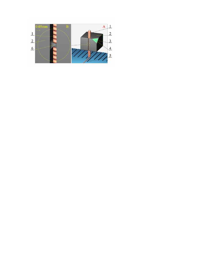
Figure 1: TF RF SQUID, made by the technique of painting, A, and a magnified view of the SQUID bridge, B. 1 – the coupling coil; 2 – the SQUID sensor body; on the angle truncated: 3 – the layer of YBa₂Cu₃O_7-δ, 4 – the substrate of Y₂BaCuO₅; 5 – the coupling coil sheave; 6 – the SQUID bridge.

These studies did not aim to develope an RF SQUID with the large inductance; such SQUIDs were a by–product of works, i. e. a consequence of painting defects that led to the disorganized geometry of a quantization loop but not to degradation of superconductive properties as well.

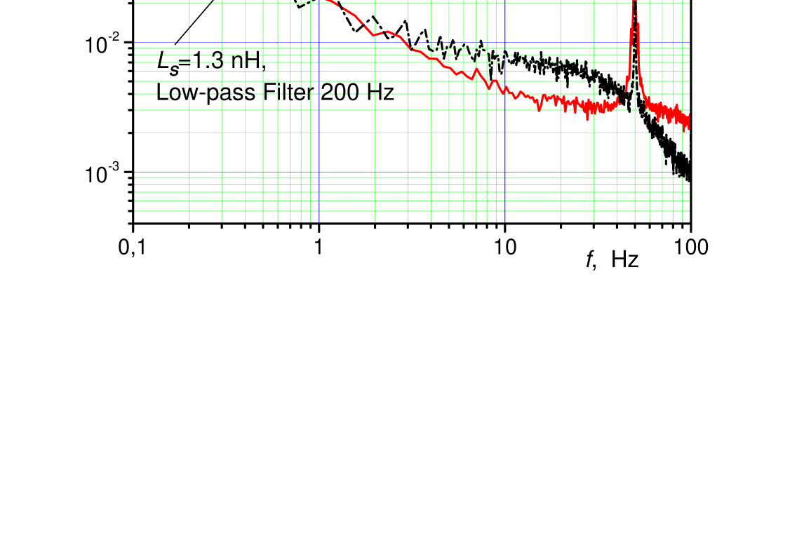
Figure 2: S. n. d. of SQUIDs with $L_{S}=1{.}3$ nH and $L_{S}=1{.}6$ nH.

It is clear now that it is precisely these good superconductive properties of the high–$T_{c}$ TFs synthesized in this way, and their high stability to degradation, that allowed us to obtain the data for s. n. d. of several large inductance SQUIDs with $L_{S}\gg L_{F}$ (see Fig. 2).
In these SQUIDs, the popular pattern of the steady state quantum interference, as it is shown in Fig. 3, was observed.

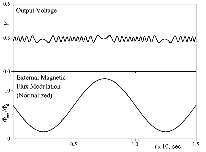
Figure 3: Typical volt–to–flux characteristic of RF SQUID having large inductance $L_{S}$ of quantization loop, obtained with sine–wave modulation of external magnetic flux (digital modeling).

Large inductance SQUIDs. Usually, SQUIDs with obvious defects of uniformity of TF, such as the unpainted sites on their surface, manifest high magnitude of quantization loop inductance, which is much higher than the calculated magnitude of geometrical SQUID–hole inductance.
In the case of biconnected samples, similar phenomenon is considered commonly as a manifestation of the percolation nature of supercurrent in ceramics with poor content of superconducting phase Verkin .
In our case, this fact can be interpreted as follows. The one–hole SQUID is not a one–inductance device; in this regard, it is similar to a two–hole Zimmerman’s SQUID Zimmerman1970 , but, unlike that, the one–hole RF SQUID should be considered as an asymmetric one, including two different loops of inductance.
The main, or the master, quantization loop is $L_{S}$ loop (see Fig. 4) located on the internal surface of the SQUID hole. When the SQUID bridge occurs in a normal resistive state under the action of pumping, the inductance $L_{S}$ joins in series the loop $L_{C}$ located on the external surface of SQUID (see Fig. 4). If there are no defects, then $L_{C}\sim L_{S}$ (see Fig. 4 A). One can see that $L_{C}$ and $L_{S}$ are connected in a subtractive polarity mode, then such a contour operates as a differential flux transformer having a small effective inductance and a low field sensitivity, as was observed in Vasiliev1995 . The defects of painting as is shown in Fig. 4 B, may yield $L_{C}\gg L_{S}$; then, the effective inductance of RF SQUID is determined by the external loop inductance $L_{C}$. The kinetic inductance, which influence in the case of thin–film is considered essential VVS , may give some contribution to the impedance of the quantization loop; in general, this aspect needs a separate research (see, also Koelle_Chesca , Sermyagin_2003 ).

Figure 4: Topology of the quantization loop of the one–hole RF SQUID. A – A defect–free high–$T_{c}$ sample. B – A sample containing non–superconductive superficial Y₂BaCuO₅ inclusions, 1; 2 – YBa₂Cu₃O_7-δ superconducting layer; $JJ$ – SQUID bridge (Josephson junction). For explanation of $L_{C}$ and $L_{S}$ see the text.

Hereinafter $L_{S}$ means the RF SQUID efficient quantization loop inductance, which can be evaluated experimentally.
For an experimental determination of RF SQUID parameters, techniques Polushkin1989_JINR_Rapid , Polushkin1990 were employed. The techniques allow one to find the SQUID inductance $L_{S}$ and its coupling coefficient $k$ between the interferometer loop and the tank circuit, with the accuracy approximately of 20$\%$. A critical current $I_{c}$ of weak link is calculated directly from the value of the hysteresis parameter $\beta=2\pi(I_{c}L_{S}/\Phi_{0})$ defined from the measuring of the amplitude and displacement of the flux–to–voltage characteristic Likharev1985 .
In this paper, experimental data for RF SQUIDs with large and very large inductances $L_{S}\gg L_{F}$, considerably exceeding the known published values Polushkin1989 , Vasiliev1990 , Il'ichev1997 , Chesca_1998 , are presented. A derivation of a new flux–resolution formula for $S_{\varphi}$ depending on $L_{S}$, which seems to be correct over the broad range $L_{S}\gg L_{F}$, is given. It is shown, by applying the relationship for $S_{\varphi}(L_{S})$, that experimental data for s. n. d. of a large inductance RF SQUID allow one to estimate a sensitivity of the RF SQUID with the loop inductance $L_{S}=L_{F}$; i. e., to actually determine a sensitivity of the RF SQUID made of a given HTS in the case of optimal quantization loop inductance.

1 Fluctuations in the Interferometer

An important inherent feature of HTS SQUIDs working at 77 K, is a high level of fluctuations. If thermal fluctuations dominate in a SQUID, a method of the Fokker–Plank equation should be applied Likharev1985 , Polushkin1989 , Chesca_1998 .
The Fokker–Plank equation is written for the probability density $\sigma(t,\varphi,v)$ to find a system at a time $t$, phase $\varphi$, and volume $v$. Knowing $\sigma(t,\varphi,v)$, it is possible to find the average of a function $F(\varphi,v)$ over the statistical ensemble by the usual way

$$\langle F(t)\rangle=\int\limits_{-\infty}^{\infty}dv\int\limits_{-\infty}^{\infty}d\varphi\sigma(t,\varphi,v)F(\varphi,v).$$ (1)

In a non–hysteretic ($\beta<1$) SQUID, only the steady state corresponding to the minimum of the Hibbs function $G$ exists, i. e., the system energy

$$G=K+U\phantom{\,\,\,=Q^{2}/2C+E_{c}[(1-\cos{\varphi})+(\varphi-\varphi_{ext})^{2}/2\beta]}$$

$$=Q^{2}/2C+E_{c}[(1-\cos{\varphi})+(\varphi-\varphi_{ext})^{2}/2\beta],\phantom{=K+U}$$ (2)

where $K$ and $U$ are the kinetic and the potential energy of the SQUID, $Q$ and $C$ are the charge and the capacity of the Josephson junction, accordingly, $E_{c}=\hbar I_{c}/2e$ is the Josephson coupling energy of the junction, $\varphi=2\pi\Phi/\Phi_{0}$, $\Phi$ is the magnetic flux coupled to the quantization loop by the relationship $\beta\sin{\varphi}=\varphi_{ext}-\varphi$, $\varphi_{ext}=2\pi\Phi_{ext}/\Phi_{0}$, and $\Phi_{ext}$ is the external magnetic flux.
A small noise yields, therefore, small phase fluctuations within this state. The probability density of finding a system in a phase space point is proportional to the Bolzmann distribution

$$\sigma\sim\exp(-G/k_{B}T).$$ (3)

If $\beta\ll 1$, it is enough to hold the last term in the potential energy expression (1), and for the dispersion of flux fluctuations one receives

$$\langle{\widetilde{\Phi}}^{2}\rangle\approx(\Phi_{0}/2\pi)^{2}\langle{\widetilde{\varphi}}^{2}\rangle\approx k_{B}TL_{S}.$$ (4)

The expression (4) permits one to estimate the interference degradation in the case of $L_{S}>L_{F}$ Likharev1985 ,

$$\langle U\rangle\approx-E_{c}\cos{\langle\varphi\rangle}\exp(-L_{S}/2L_{F}),$$ (5)

where $L_{F}\equiv(\Phi_{0}/2\pi)^{2}(k_{B}T)^{-1}$; at $T=4$ K, $L_{F}=2\cdot 10^{-9}$ H.
The relationship (5) is valid for a nonhysteretic mode the criterion of which is the validity of the inequality for the hysteretic SQUID parameter, $\beta<1$, by the former theories which have been offered prior to the discovery of HTS.
However as early as in 1975, in the theoretical analysis of an RF SQUID it was noticed Khlus_Kulik , that in the case of large fluctuations, i. e., when the Josephson coupling energy $E_{c}$ of junction is less than the average thermal energy ($\Gamma=(k_{B}T/E_{c})>1$), the SQUID is nonhysteretic. B. Chesca Chesca_1998 and Ya. Greenberg Greenberg_1999 have come to a similar conclusion developing an RF SQUID theory applicable to the case of high fluctuations and which conclusions are supported by the known experimental data. In particular, according to the Chesca–Greenberg theory, an RF SQUID is non hysteretic under conditions of high fluctuations, up to the hysteresis parameter value of $\beta\leq 3$. Thus, there is a basis for applying a simple form (5) of the interference supression dependence on inductance to estimate a noise of the SQUID with high inductance $L_{S}$.
The components of a net noise of an interferometer that determine its sensitivity, are as follows Rogachevskiy1993 , Koelle :

• self–noise, or internal noise of the sensor (SQUID) of the interferometer;

• the noise of the tank circuit coupled inductively to the SQUID;

• the noise of a feeder connecting the tank circuit to the preamplifier; if the preamplifier is placed outside the dewar, the ends of the feeder have a temperature difference causing the noise.

• Noises of the first amplifier stage and of a resistor in the feedback loop. They can be reduced sufficiently by cooling the first stage. It is profitable, from the view point of increasing sensitivity, in the case of low–$T_{c}$ SQUIDs having the own sensor noise much lower than the rest noise sources. For high–$T_{c}$ SQUIDs operating at liquid nitrogen temperature, the sensor noise is not much less than the noise of electronics.

• The external noise. To estimate the interferometer sensitivity, it should be minimized. The best way to minimize external influences is to apply a superconducting shield the SQUID sensor is placed into. For this purpose, the high–$T_{c}$ shield should have a low level of the self–noise. This condition is met when the high–$T_{c}$ shield has a high enough value of the penetrating field Polushkin_Buev . Nevertheless, employing an ordinary ferromagnetic shielding provides a relevant solution.

The internal noise of the SQUID sensor is defined by Josephson junction properties, and by magnetic flux fluctuations having dispersion (4). Self–noise of HTS–based Josephson junction can be low enough; the higher the critical current density, the lower the self–noise. In YBCO systems, it is possible to achieve high values of the pinning force Vuong_1994 , Vasiliev1995 , Koelle , which guarantees high values of critical current density in the $ab$–plane of a YBCO crystal cell, and an acceptably low level of excess $1/f$ noise as well. A theoretical estimate of the internal noise level and the maximum inductance of the RF SQUID quantization loop can be carried out in a simple way Polushkin1989_JINR_Rapid . For an RF SQUID with the inductance $L_{S}=10^{-10}$ H the estimate of s. n. d. at the temperature 77 K gives

$$S_{\varphi}=10^{-5}\mbox{\,}\Phi_{0}/\mbox{Hz}^{1/2}.$$ (6)

According to Polushkin1989_JINR_Rapid , quantum interference in the RF SQUID is hardly observed if the value of the RF SQUID threshold inductance $L_{max}$ is exceeded

$$L_{S}>L_{max}=\Phi^{2}_{0}/k_{B}T=4\cdot 10^{-9}\mbox{\,H.}$$ (7)

At that time (1989), these conclusions were not experimentally proven probably due to poor quality of HTS ceramics, which did not allow simple handling of SQUIDs. At present, the sensitivity level (6) is successfully achieved in high–$T_{c}$ RF SQUIDs produced on the basis of modern thin film technologies Zhang . In its turn, studying of the SQUIDs made by using the thick–film technique, have a confirmation and specification of these estimates as well. Thus, according to the estimate (7), for the high–$T_{c}$ SQUIDs operated at $77$ K, a wide enough inductance range including even “He–values” up to several nH is available. According to the estimate (6), in the case of the optimum quantization loop inductance, the interferometer sensor self–noise is appreciably below the tank circuit noise and the noise of the “warm” preamplifier, as well as in the case of the low–$T_{c}$ RF SQUIDs. As evident from what follows, the estimates of the maximum sensitivity of the RF SQUIDs with the optimum quantization loop inductance, carried out on the basis of the experimental s. n. d. data for large inductance SQUIDs, agree well with (6).

2 Dual SQUID

Let us introduce a concept of a SQUID which is dual to the RF SQUID with a large quantization loop inductance. A dual SQUID is a SQUID with the same weak link properties as a SQUID with a high inductance value, but with the optimum quantization loop inductance value equal to $L_{F}$. In a formal way, it is possible to obtain a dual SQUID from a large inductance RF SQUID by deforming the quantization loop to reduce its inductance down to $L_{F}$, preserving the weak link parameters. Since the noise of the SQUID sensor with the large inductance $L_{S}\gg L_{F}$ is determined, in accordance with (5), by the “Debye” factor $\exp{(L_{S}/2L_{F})}$ only, it is possible to carry out a simple theoretical estimate of the sensitivity of the appropriate dual SQUID, and, thus, to estimate the suitability of the given HTS for a high sensitivity SQUIDs building.

3 About Scaling Behaviour of the Interferometer Sensor Noise

Let the total interferometer spectral noise energy density (s. n. e. d.) $S_{\epsilon}$ be determined in a general way, as usual (see, for example Polushkin1993 , Sloggett1993 ), by its fluctuation components $S_{\epsilon i}$, $i=1,2...,n$, which are considered uncorrelated

$$S_{\epsilon}=S_{\epsilon 1}+S_{\epsilon 2}+...+S_{\epsilon n}.$$ (8)

Let, for example, $S_{\epsilon 1}$ be a s. n. e. d. of the SQUID sensor, $S_{\epsilon 2}$ – s. n. e. d. of the tank circuit coupling inductively to the SQUID, $S_{\epsilon 3}$ – s. n. e. d. of the feeder, $S_{\epsilon 4}$ – s. n. e. d. of the first preamplifier stage. In the best case, the components specified differ from each other no more than one order of magnitude Koelle . Let the s. n. e. d. of the SQUID sensor be written as

$$S_{\epsilon 1}=S_{\epsilon 1}(L_{S})=S_{\epsilon d}\cdot K(L_{S}),$$ (9)

where $S_{\epsilon d}$ is the value of the SQUID s. n. e. d. (energy resolution) depending on the absolute temperature and weak link parameters, a critical current and a normal resistance, and also, maybe, on Josephson junction capacity, but independent of $L_{S}$, and $K(L_{S})$ is a dimensionless scale factor depending monotonously on $L_{S}$. It is supposed that all other components $S_{\epsilon i}$, $i\neq 1$, do not depend on $L_{S}$. Thus, $S_{\epsilon d}$ is s. n. e. d. of the SQUID sensor with a rather small inductance. Let now $K(L_{S})$ increases, together with $L_{S}$, and the remaining parameters in (8) remain constant, so that, when $L_{S}\gg L_{F}$, one could obtain $S_{\epsilon 1}\gg S_{\epsilon i}$, $i=2,3,4$. Hence, from (8) and (9), it evidently follows:

$$S_{\epsilon}\simeq S_{\epsilon 1}(L_{S})=S_{\epsilon d}\cdot K(L_{S}).$$ (10)

The last equation (10) reflects two important facts. First, in the case of high inductance of the quantization loop, the interferometer noise is determined mainly by the SQUID sensor noise. Second, the interferometer s. n. e. d. at the high values of inductance of the quantization loop is proportional to the s. n. e. d. of the SQUID sensor with the same weak link parameters, but a small quantization loop inductance. If the functional dependence of the $K(L_{S})$ is known, in the presence of the experimental data for $S_{\epsilon}$ of a SQUID with a large inductance, the relationship (10) allows one to determine energy resolution $S_{\epsilon}$ of a SQUID with the same weak link but with optimum inductance value. Let us obtain now a relationship between the s. n. d. $S_{\varphi}$ of a SQUID with a large quantization loop inductance and the s. n. d. $S_{\varphi d}$ of a SQUID with an optimum quantization loop inductance. By definition, the SQUID s. n. e. d. $S_{\epsilon}$ (with a dimension of the action, $[S_{\epsilon}]=\mbox{J}\cdot\mbox{Hz}^{-1}$) is connected with the s. n. d. $S_{\varphi}$, $[S_{\varphi}]=\Phi_{0}/\mbox{Hz}^{1/2}$, by the relationship

$$S_{\epsilon}=\frac{S^{2}_{\varphi}}{2L_{S}}$$ (11)

It has been experimentally proved Polushkin1989 , that the optimum quantization loop inductance value is close to $L_{F}$. Taking into account the equation

$$S_{\epsilon d}=\frac{S^{2}_{\varphi d}}{2L_{F}},$$ (12)

and, combining (10), (11), (12), it is easy to obtain the useful estimate

$$S_{\varphi d}\simeq S_{\varphi}\cdot\left[\frac{L_{F}}{L_{S}\cdot K(L_{S})}\right]^{1/2}{,}\mbox{ }L_{S}\gg L_{F}.$$ (13)

Let us regard the (13) as s. n. d. of dual SQUID, i. e.

$$S_{\varphi\mbox{ }dual}\simeq S_{\varphi}\cdot\left[\frac{L_{F}}{L_{S}\cdot K(L_{S})}\right]^{1/2}{,}\mbox{ }L_{S}\gg L_{F}.$$ (14)

Assuming that $K(L_{S})=\exp{[(L_{S}/2L_{F})-1/2]}$, we obtain

$$S_{\varphi\mbox{ }dual}\simeq S_{\varphi}\cdot\left(\frac{L_{F}}{L_{S}}\right)^{1/2}\cdot\exp{\left[\frac{1}{4}\cdot\left(1-\frac{L_{S}}{L_{F}}\right)\right]},\mbox{ }L_{S}\gg L_{F}.$$ (15)

Thus, we have obtained the relationship (15) which links $S_{\varphi}$ of a SQUID with a large quantization loop inductance value of $L_{S}\gg L_{F}$, with $S_{\varphi\mbox{ }dual}$ of a dual SQUID with the optimum quantization loop inductance value of $\sim L_{F}$. This relation allows one to estimate, using the experimental data, the suitability of a given high–$T_{c}$ material, from which the large inductance SQUIDis was made, for building high–sensitive interferometers.
In Table 1, the experimental data for real RF SQUID parameters are given, including loop quantization inductances $L_{S}$, coupling coefficient $k$ measured by the technique Polushkin1989_JINR_Rapid , and the values of SQUID hysteresis parameter $\beta$ and s. n. d. $S_{\varphi}$, measured at pumping frequency indicated in the last column. The critical current of contact $I_{c}$ is calculated then from $\beta=2\pi L_{S}I_{c}/\Phi_{0}$, and the flux sensitivity $S_{\varphi\mbox{ }dual}$ for the appropriate dual SQUID is calculated from (15). The RF SQUID transfer function grows with the growth of the pumping frequency $f$ as $f^{1/2}$, and RF SQUID s. n. d. decreases with the same rate; it is necessary to take into account these dependencies when comparing quality of SQUIDs functioning at different pumping frequencies Kurkijarvi_1986 . An appropriate technique of SQUID signal characteristics ranging, by the pumping frequency, will be considered elsewhere Sermyagin_2003 .

Table 1:

#	$L_{S}$, nH	$k$	$\beta$	$I_{c}$, $\mu$A	$S_{\varphi}$, $\Phi_{0}$/Hz1/2	$S_{\varphi\mbox{ }dual}$, $\Phi_{0}$/Hz1/2	$f_{L_{t}C_{t}}$, MHz
1	1.3	0.12	18	4.6	$3{.}1\cdot 10^{-3}$	$4{.}6\cdot 10^{-5}$	$\sim 20$
2	1.61	0.28	52	8.2	$7{.}3\cdot 10^{-3}$	$4{.}6\cdot 10^{-5}$	—”—
3	2	0.15	21	3.3	–	–	—”—
4	2.76	0.22	60	7.2	$1,5\cdot 10^{-3}$	$4{.}3\cdot 10^{-7}$	—”—
5	3.8	–	–	–	0.1	$1{.}9\cdot 10^{-6}$	—”—
6	6.6	0.101	7	0.35	$\sim 0{.}1$	$\sim 1{.}7\cdot 10^{-9}$	—”—
7	24	0.075	–	0.04	–	–	—”—
8	0.51	–	2	–	$10^{-3}$	$1{.}6\cdot 10^{-4}$	—”— Polushkin1989
9	0.7	–	–	–	$3\cdot 10^{-4}$	$2{.}7\cdot 10^{-5}$	25 Il'ichev1997
10	0.45	–	1.5	0.835	$7\cdot 10^{-5}$	$1{.}4\cdot 10^{-5}$	300 Chesca_1998
11	0.9	–	2.25	0.835	$5{.}66\cdot 10^{-4}$	$2{.}7\cdot 10^{-5}$	—”—

4 A Comment on the Table

For SQUIDs $\#\#$1$\div$7, the experimental data obtained by the author of the present paper are given, other data are taken from references.
The data are not complete; s. n. d. for $\#$2 and $\#$7 are not retained. Parameters for $\#$7 were defined with an error difficult to estimate, therefore the real value of $L_{S}$ could differ from the specified; most likely it was smaller. Data of $k$, $\beta$, and $I_{c}$ for $\#$5 are lost as well; for SQUIDs $\#\#$8 $\div$11, the reader is kindly addressed to the references. However, the data omitted are not crucial for conclusions of the qualitative theory submitted. It can be seen that in the range $L_{S}<2$ nH, for $S_{\varphi\mbox{ }dual}$, real values can be obtained corresponding to the self–noise of the optimum SQUID made from the sertain HTS. For $\#$8, the value of $S_{\varphi\mbox{ }dual}\sim 10^{-4}$  $\Phi_{0}$/Hz^1/2 is not very high, which is usual for bulk SQUIDs made of ceramics typical to the initial period of HTS research in the late eighties, though already sufficient for applications. $\#$1 and $\#$2 are created by the painting method, and by far overcome the psychological barrier of $10^{-4}$ $\Phi_{0}$/Hz^1/2, into the value area of units $10^{-5}$ $\Phi_{0}$/Hz^1/2, close to the best theoretical estimate (6), near which the thin film RF SQUIDs $\#$9, $\#$10 and $\#$11 are situated; these latter two were operated at the pumping frequency of 300 MHz. Hence, sample $\#$10 has the weak link quality close to our samples $\#$1 and $\#$2.
For SQUIDs whith a very large inductance $L_{S}>2$ nH, the extrapolation to the dual SQUIDs does not work thus far due the very low level of the noise predicted. It means, that in RF SQUIDs with a very large quantization loop inductance values, quantum interference is suppressed not so strongly as it follows from the simple formula (15); our assumption of the suppression character (5) of quantum interference with growth of inductance $L_{S}$, appears inexact in this area. One of the possible ways of solving this problem consists in a consequent account of the reduction phenomena of the RF SQUID transfer function, with the fluctuation level growing Il'ichev1997 , Chesca_1998 , Greenberg_1999 , Enpuku1994 ; this concerns both thermal and quantum fluctuations Sermyagin_1997_1 . The general conception is that with the reduction of SQUID transfer function, the SQUID sensitivity decreases both to the useful signal and to fluctuations.
The interference in $\#$6 and $\#$7 was observed, despite of extremely high SQUIDs inductance values $L_{S}$ and small values of critical current $I_{c}$. These values were much less the fluctuation current value of 3 $\mu$A, which is considered the lower value of a critical current for isolated HTS–based junction at 77 K, admitting the observing of the quantum interference.

5 Conclusions

The fluctuation inductance $L_{F}$ is not an upper limit of the quantization loop inductance, exceeding which the quantum interference becomes unobservable and SQUID ceases to operate. More likely, one should consider $L_{F}$ as a quality criterion of the SQUID, actually as an optimum value of the quantization loop inductance. So far the large inductance SQUIDs with $L_{S}\gg L_{F}$ were considered not applicable as supersensitive magnetic flux sensors, due to a large level of their self–noise. However, this feature allows one to receive an estimate of the maximum sensitivity of the RF SQUID with an optimum inductance of the quantization loop and made of appropriate HTS. The obtained estimate (15) of the $S_{\varphi}(L_{S})$ dependence based on a rough model (5), appears true, if compared to the obtained experimental data for the large inductance values of $2\cdot 10^{-9}>L_{S}>10^{-10}$, H. However, an interpretation of the experimental data for higher inductance values of $L_{S}>2\cdot 10^{-9}$ H needs a new approach (see e. g. Sermyagin_2003 ).

6 Acknowledgments

The results presented could not be obtained without an intensive development of the painting on method and HTS–sample investigations carried out by Prof. N.V. Vuong and Dr. E.V. Pomyakushina (Raspopina), under supervision of Prof. B.V. Vasiliev. Also, I wish to thank Dr. M.B. Miller and O.Yu. Tokareva for their support and help.

References

- [1] N.V. Vuong, E.V. Raspopina, and B.T. Huy, Supercond. Sci. Technol. 6 (1993) 453.
- [2] M. Murakami, Supercond. Sci. Techn. 5 (1992) 185.
- [3] N.V. Vuong, E.V. Raspopina, V.V. Scugar, N.M. Vladimirova, N.A. Yakovenko, and I.A. Stepanova, Physica C 233 (1994) 263.
- [4] B.V. Vasiliev, N.V. Vuong, E.V. Raspopina, and A.V. Sermyagin, Physica C 250 (1995) Nos. 1/2, 1.
- [5] B.I. Verkin, I.M. Dmitrenko, V.M. Dmitriev, V.V. Kartsovnik, A.G. Kozyr, V.A. Pavlyuk, G.M. Tsoi, V.I. Shnyrkov, Fiz. Nizk. Temp. 14, (1988) 34 .
- [6] J.E. Zimmerman, P. Thiene, J.T. Harding, J. Appl. Phys. 41 (1970) 1572.
- [7] V.V. Shmidt, Vvedenie v fiziku sverkhprovodnikov, Nauka Press, Moscow (1982) ( in Russian).
- [8] A.I. Braginski, K. Barthel, B. Chesca, Y. Greenberg, R. Kleiner, D. Koelle, Y. Zhang, and X. Zeng, Physica C 341–348 (2000) 2555.
- [9] A.V. Sermyagin (manuscript in preparation).
- [10] V.N. Polushkin, B.V. Vasiliev, JINR Rapid Comm. 1[34] (1989) 55.
- [11] V.N. Polushkin, Izmereniya, Kontrol’, Avtomatizatsiya 3[75] (1990) 14.
- [12] K.K. Likharev, Introduction to the Dynamics of Josephson Transition, Nauka Press, Moscow (1985) (in Russian).
- [13] V.N. Polushkin, JINR Preprint R13–89–201 Dubna (1989).
- [14] Vasiliev B.V., Polushkin V.N., Pryb. i Tekhn. Eksp. 3 (1990) 182.
- [15] E. Il´ichev, V.M. Zakosarenko, R.P.J. Ijsselstejn, and V . Schultze, J. Low Temp. Phys. 106 (1997) Nos. 3/4, 503.
- [16] B. Chesca, J. Low Temp. Phys. 110 (1998) Nos. 5/6, 963.
- [17] V.A. Khlus and I.O. Kulik, Zh. Teckhn. Fiz. XLV (1975) 449.
- [18] Ya.S. Greenberg, J. Low Temp. Phys. 114 (1999) Nos. 3/4 297.
- [19] B.M. Rogachevskiy, Avtometriya N1 (1993) 3.
- [20] D. Koelle, R. Kleiner, F. Ludwig, E. Dantsker and John Clarke, Rev. Mod. Phys. 71 (1999) No. 3, 631.
- [21] V.N. Polushkin, A.R. Buev, JINR Preprint R13–92–42 Dubna (1992).
- [22] Y. Zhang, W. Zander, J. Shubert, F. Rüders, H. Soltner, M. Banzet, N. Wolters, X.H. Zeng, and A.I. Braginskij, Appl. Phys. Lett. 71 (1997) 704.
- [23] V.N. Polushkin, Sverkhprovodymost’: Fizika, Khimiya, Tekhnologiya 6 (1993) N5, 895.
- [24] J. Sloggett, D.L. Dart, C.P. Foley, R.A. Binks, N. Savvides and A. Katsarov, Supercond. Sci. Technol. 7 (1994) 260.
- [25] Reino I. Kernen and Juhani Kurkijrvi, J. Low Temp. Phys. 65 (1986) Nos. 3/4, 279.
- [26] K. Enpuku, G. Tokita, and T. Maruo, J. Appl. Phys. 76 (1994) 8180.
- [27] A.V. Sermyagin, J. Low Temp. Phys. 106 (1997) Nos. 3/4, 533.