Analysis of the radio-frequency single-electron transistor with large quality factor

Abstract

We have analyzed the response and noise-limited sensitivity of the radio-frequency single-electron transistor (RF-SET), extending the previously developed theory to the case of arbitrary large quality factor $Q$ of the RF-SET tank circuit. It is shown that while the RF-SET response reaches the maximum at $Q$ roughly corresponding to the impedance matching condition, the RF-SET sensitivity monotonically worsens with the increase of $Q$. Also, we propose a novel operation mode of the RF-SET, in which an overtone of the incident rf wave is in resonance with the tank circuit.

The problem of relatively small bandwidth of the conventional single-electron transistor[2, 3] (SET) due to its large output resistance, has been solved for many applications by the invention[4] of the radio-frequency SET (RF-SET), which in many instances has already replaced the traditional SET setup. The principle of the RF-SET operation is somewhat similar to the operation of the radio-frequency superconducting quantum interference device [5] (RF-SQUID) and is based on the microwave reflection [4, 6, 7, 8] from a tank circuit containing the SET (Fig. 1), which affects the quality factor ($Q$-factor) of the tank; another possibility is to use the transmitted wave.[9, 10] The wide bandwidth of the RF-SET is due to the signal propagation by the microwave instead of charging the output wire, while the tank circuit provides a better match between the cable wave impedance $R_{0}=50\,\Omega$ and much larger SET resistance ($\sim 10^{5}\,\Omega$).

The RF-SET bandwidth over 100 MHz has been demonstrated [4] using the microwave carrier frequency $\omega/2\pi=1.7$ GHz and relatively low $Q$-factor $Q\simeq 6$. However, in the present-day experiments the bandwidth is typically about 10 MHz because of lower carrier frequency (to reduce amplifier noise) and higher $Q$-factor (as an example, the bandwidth of 7 MHz for $\omega/2\pi=332$ MHz and $Q>20$ has been reported in Ref. [7]).

Since the SET sensitivity is limited by the $1/f$ noise only at frequencies below few kHz, the RF-SET typically operates in the frequency range of shot-noise limited sensitivity of the SET.[11, 12] The RF-SET charge sensitivity of $3.2\times 10^{-6}e/\sqrt{\mbox{Hz}}$ ($4.8\hbar$ in energy units) at 2 MHz has been reported in Ref. [7]. Even though this value still contains comparable contributions from the SET and amplifier noises, the pure shot-noise-limited sensitivity seems to become achievable pretty soon.

In spite of significant experimental RF-SET activity, we are aware of only few theoretical papers on the RF-SETs. The basic theory of the shot-noise-limited sensitivity of the RF-SET has been developed in Ref. [13]. A similar theory has been applied to the analysis of the sensitivity of the RF-SET-based micromechanical displacement detector.[14, 15] Some theoretical analysis of the transmission-type RF-SET can be found in Ref. [10].

In this letter we extend the theory of Ref. [13] to the case of arbitrary large $Q$-factor of the tank circuit, removing the assumption of $Q$ being much smaller than the impedance-matching value. (While this condition was satisfied in the first experiment,[4] it is strongly violated in the present-day experiments.) We calculate the response and sensitivity of the normal-metal RF-SET and find the optimal values numerically. Besides the usual case of the carrier wave in resonance with the tank circuit, we also consider the regime of a resonant overtone and find a comparable RF-SET performance in this case.

FIG. 1.: Schematic of the RF-SET.

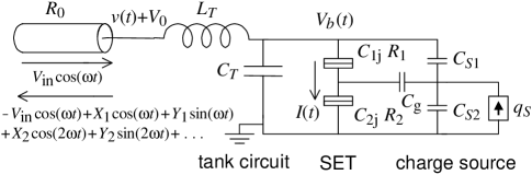
We consider a SET (Fig. 1) consisting of two tunnel junctions with capacitances $C_{1j}$ and $C_{2j}$ and resistances $R_{1}$ and $R_{2}$. The measured charge source $q_{S}$ has the capacitance $C_{S}=C_{S1}+C_{S2}$ and is coupled to the SET via capacitance $C_{g}$. Assuming constant $q_{S}$ (neglecting backaction), the SET can be reduced to the effective double-junction SET with capacitances $C_{1}=C_{1j}+C_{g}C_{S1}/(C_{g}+C_{S})$, $C_{2}=C_{2j}+C_{g}C_{S2}/(C_{g}+C_{S})$ and background charge $q_{0}=q_{00}+q_{S}C_{g}/(C_{g}+C_{S})$, where $q_{00}$ is the initial contribution. We will calculate the RF-SET response and sensitivity in respect to $q_{0}$, while the corresponding quantities in respect to the measured charge $q_{S}$ differ by the factor $C_{g}/(C_{g}+C_{S})$.

The current $I(t)$ through the SET affects the quality factor of the tank circuit consisting of the capacitance $C_{T}$ and inductance $L_{T}$. In the linear approximation the SET can be replaced by an effective resistance $R_{d}$, and the total (“loaded”) quality factor $Q_{L}=(1/Q+1/Q_{SET})^{-1}$ has contributions from the “unloaded” $Q$-factor $Q=\sqrt{L_{T}/C_{T}}/R_{0}$ and damping by the SET: $Q_{SET}=R_{d}/\sqrt{L_{T}/C_{T}}$. For the incoming voltage wave ${\hat{V}}_{in}\exp({\rm i}\omega t)$, the reflected wave $\alpha{\hat{V}}_{in}\exp({\rm i}\omega t)$ depends on the reflection coefficient $\alpha=(Z-R_{0})/(Z+R_{0})$, where $Z={\rm i}\omega L_{T}+({\rm i}\omega C_{T}+1/R_{d})^{-1}$; close to the resonance, $\omega\approx\omega_{0}=(L_{T}C_{T})^{-1/2}$, it can be approximated as $Z\approx L_{T}/C_{T}R_{d}+2{\rm i}(L_{T}/C_{T})^{1/2}\Delta\omega/\omega_{0}$, $\Delta\omega\equiv\omega-\omega_{0}$. Since an increment of the measured charge $q_{S}$ leads to an increment of $R_{d}$, the RF-SET response is proportional to $d\alpha/dR_{d}$. However, the amplitude ${\hat{V}_{b}}={\hat{V}}_{in}(Z+R_{0})({\rm i}\omega C_{T}+1/R_{d})/2$ of the SET bias voltage oscillations should be determined by the Coulomb blockade threshold; so a more representative quantity is

$$\frac{d\alpha}{dR_{d}}\frac{\hat{V}_{in}}{\hat{V}_{b}}\approx\frac{-{\rm i}R_{0}}{R_{d}^{2}}\,\frac{Q}{1+Q^{2}R_{0}/R_{d}}\,\frac{1}{1+2{\rm i}Q_{L}\Delta\omega/\omega_{0}}.$$ (1)

This equation shows that the RF-SET response reaches the maximum at $Q=(R_{d}/R_{0})^{1/2}$, which is the case of matched impedances at resonance, $Z\approx R_{0}$, and corresponds to the condition $Q=Q_{SET}=2Q_{L}$.

The linear analysis can only be used as an estimate because of the significant nonlinearity of the SET $I-V$ dependence. For the full analysis we use the differential equation [13] $\ddot{v}/\omega_{0}^{2}+\dot{v}/Q\omega_{0}+v=2(1-\omega^{2}/\omega_{0}^{2})V_{in}\cos{\omega t}-R_{0}[I(t)-\langle I\rangle]$, where $v(t)=V_{in}\cos\omega t+V_{out}(t)$ is the voltage at the end of the cable with subtracted dc component $V_{0}$ (see Fig. 1; do not use complex representation any more). The SET current $I(t)$ and its average value $\langle I\rangle$ are found self-consistently from the SET bias voltage $V_{b}(t)=V_{0}+v(t)+[2V_{in}\omega\sin{\omega t}+\dot{v}(t)]\,Q/\omega_{0}$ using the “orthodox” model[2] and assuming continuous SET current ($\omega\ll I/e$).

In the steady state the reflected wave can be represented as $V_{out}(t)=-V_{in}\cos{\omega t}+\sum_{n=1}^{\infty}[X_{n}\cos{n\omega t}+Y_{n}\sin{n\omega t}]$ and the coefficients $X_{n}$ and $Y_{n}$ can be calculated as

$$X_{n}=\{R_{0}Q[n\tilde{\omega}\,a_{n}-Q(1-n^{2}\tilde{\omega}^{2})b_{n}]+2Q^{2}(1-\tilde{\omega}^{2})^{2}$$ (2)

$$\hskip 28.45274pt\times V_{in}\delta_{1n}\}/[n^{2}\tilde{\omega}^{2}+Q^{2}(1-n^{2}\tilde{\omega}^{2})^{2}],$$ (3)

$$Y_{n}=\{-R_{0}Q[n\tilde{\omega}\,b_{n}+Q(1-n^{2}\tilde{\omega}^{2})a_{n}]+2Q\tilde{\omega}(1-\tilde{\omega}^{2})$$ (4)

$$\hskip 28.45274pt\times V_{in}\delta_{1n}\}/[n^{2}\tilde{\omega}^{2}+Q^{2}(1-n^{2}\tilde{\omega}^{2})^{2}],$$ (5)

$$a_{n}=2\langle I(t)\sin{n\omega t}\rangle,\,\,\,b_{n}=2\langle I(t)\cos{n\omega t}\rangle,$$ (6)

where $\tilde{\omega}\equiv\omega/\omega_{0}$, $\delta_{1n}$ is the Kronecker symbol, and averaging is over the oscillation period, while $I(t)$ is determined by the SET voltage $V_{b}(t)=V_{0}+2Q\tilde{\omega}V_{in}\sin{\omega t}+\sum_{n=1}^{\infty}[(X_{n}+Qn\tilde{\omega}Y_{n})\cos{n\omega t}+(Y_{n}-Qn\tilde{\omega}X_{n})\sin{n\omega t}]$. Notice that the linear approximation corresponds to neglecting the contribution of overtones ($n\geq 2$); then $R_{d}=\pi A/[\int_{0}^{2\pi}I(V_{0}+A\sin{x})\sin{x}\,dx]$, where $A$ is the amplitude of $V_{b}$ oscillations, $V_{b}(t)=V_{0}+A\sin(\omega t+\phi)$, while there is no effective reactance contribution due to SET current. We used the self-consistent linear approximation as a starting point for the iterative solution of Eqs. (3)–(6).

The RF-SET response in respect to monitoring the quadrature component $X_{n}$ can be defined as a derivative $dX_{n}/dq_{0}$ (similarly, $dY_{n}/dq_{0}$ for $Y_{n}$ monitoring). Other experimentally relevant definitions are for monitoring the optimized phase-shifted combination $X_{n}\cos\varphi+Y_{n}\sin\varphi$ or the reflected wave amplitude; however, in the cases considered below there is only one leading quadrature, so different definitions practically coincide.

The corresponding noise-limited sensitivity (minimal detectable charge for the measurement bandwidth $\Delta f$) is defined as $\delta q_{0}/\sqrt{\Delta f}=\sqrt{S_{Xn}}/|dX_{n}/dq_{0}|$ (similarly, $\sqrt{S_{Yn}}/|dY_{n}/dq_{0}|$), where the low-frequency spectral densities $S_{Xn}$ and $S_{Yn}$ of quadrature fluctuations are

$$S_{Xn}=c_{n}^{\,2}\langle S_{I}(t)\sin^{2}n\omega t\rangle+d_{n}^{\,2}\langle S_{I}(t)\cos^{2}n\omega t\rangle$$ (7)

$$\hskip 28.45274pt-c_{n}d_{n}\langle S_{I}(t)\sin 2n\omega t\rangle,$$ (8)

$$S_{Yn}=d_{n}^{\,2}\langle S_{I}(t)\sin^{2}n\omega t\rangle+c_{n}^{\,2}\langle S_{I}(t)\cos^{2}n\omega t\rangle$$ (9)

$$\hskip 28.45274pt+c_{n}d_{n}\langle S_{I}(t)\sin 2n\omega t\rangle,$$ (10)

where $c_{n}=(2R_{0}Qn\tilde{\omega})/[n^{2}\tilde{\omega}^{2}+Q^{2}(1-n^{2}\tilde{\omega}^{2})^{2}]$, $d_{n}=c_{n}Q(1-n^{2}\tilde{\omega}^{2})/n\tilde{\omega}$, $S_{I}(t)$ is the low-frequency spectral density of the SET shot noise [12] with the time dependence due to oscillating bias voltage, and the averaging is over the period $2\pi/\omega$.

FIG. 2.: (a) RF-SET response and (b) sensitivity as functions of the $Q$-factor in the maximum response (MR) and optimal sensitivity (OS) modes. $T=0.01\,e^{2}/C_{\Sigma}$, $R_{\Sigma}/R_{0}=2000$, $\omega=\omega_{0}$.

Figure 2 shows the numerically calculated RF-SET response and sensitivity as functions of the “unloaded” $Q$-factor for a symmetric SET, [16] $C_{1}=C_{2}=C_{\Sigma}/2$, $R_{1}=R_{2}=R_{\Sigma}/2$, with $R_{\Sigma}=100\,\mbox{k}\Omega$ at temperature $T=0.01e^{2}/C_{\Sigma}$ for the case of resonant carrier frequency, $\omega=\omega_{0}$. Both the response and sensitivity are shown in respect to the quadrature $X_{1}$ since all other components are small. The RF-SET performance is optimized over the wave amplitude $V_{in}$ and the charge $q_{0}$ to provide either maximum response (MR mode; solid lines) or optimized sensitivity (OS mode; dashed lines). [17] We show the results for two values of the dc bias voltage $V_{0}$. The case $V_{0}=0$ provides the best MR response and the best OS sensitivity, and corresponds to the symmetric SET operation in respect to positive and negative bias voltages (the SET $I-V$ curve is symmetric even for nonzero $q_{0}$). The other shown value $V_{0}=0.5e/C_{\Sigma}$ represents a typical case when only one branch of the SET $I-V$ curve is used, and corresponds to the plato-like region[13] of the response and sensitivity dependences on $V_{0}$.

As one can see from Fig. 2(a), the maximum RF-SET response is achieved at $Q$-factors (somewhat different in different regimes) comparable to the rough estimate $(R_{\Sigma}/R_{0})^{1/2}\simeq 45$. However, unlike in the linear model, this maximum does not correspond to the exact impedance matching. For example, the impedance matching (minimum of reflection) occurs at $Q\simeq 100$ for the upper curve in Fig. 2(a) and at $Q\simeq 80$ for the curve second from the top, while for two lower curves (OS mode) it does not occur at all in a reasonable range of $Q$.

In contrast to the response behavior, the RF-SET sensitivity [Fig. 2(b)] monotonically worsens with $Q$. Qualitatively, this happens because the noise $S_{X1}$ in Eq. (8) is proportional to $Q^{2}$, while the response does not grow as fast as $Q$. At low $Q$ the OS sensitivity is fitted well by the analytical result [13] $\delta q_{0}\simeq 2.65e(R_{\Sigma}C_{\Sigma}\Delta f)^{1/2}(TC_{\Sigma}/e^{2})^{1/2}$ for $V_{0}=0$ and $\delta q_{0}\simeq 3.34C_{\Sigma}(R_{\Sigma}T\Delta f)^{1/2}$ for the asymmetric operation (shown by dotted lines). However, at realistic $Q$-factors $\delta q_{0}$ is significantly larger (by about 50% at $Q=50$ for data in Fig. 2). Another interesting observation from Fig. 2 is that the response in the MR mode is only moderately ($\sim 30\%$) better than in the OS mode.

FIG. 3.: Dependence of (a)–(b) RF-SET response and (c)–(d) sensitivity on temperature $T$ in the MR and OS modes for several $Q$-factors. $V_{0}=0$, $R_{\Sigma}/R_{0}=2000$, and $\omega=\omega_{0}$.

Figure 3 shows the temperature dependence of the RF-SET response and sensitivity in the MR and OS modes. Even though the low-$T$ analytical formula for the OS sensitivity (above) works well only for small $Q$, the $T^{1/2}$ dependence at $T\lesssim 0.05e^{2}/C_{\Sigma}$ remains valid for large $Q$-factors (at very small $T$ the OS sensitivity is limited by the neglected here contribution from cotunneling processes [11, 18]). The OS response practically does not depend on temperature at $T\lesssim 0.05e^{2}/C_{\Sigma}$. The performance in the MR mode saturates below $T\simeq 0.03e^{2}/C_{\Sigma}$.

FIG. 4.: (a) RF-SET response and (b) sensitivity in the regimes when the second or third overtone of the incident rf wave is in resonance with the tank circuit. $T=0.01\,e^{2}/C_{\Sigma}$, $R_{\Sigma}/R_{0}=2000$.

So far we have been considering the usual case $\omega=\omega_{0}$. In spite of significant SET $I-V$ nonlinearity (the SET nonlinearity has been recently used [19] for rf mixing), the contribution of overtones in this case is small because they are off resonance. Even though the formally calculated sensitivities in respect to overtones are comparable to the $X_{1}$ sensitivity (worse by less than two times for $n=2$ and 3), the responses are much smaller and therefore monitoring of overtones is impractical. However, the contribution of $n$th overtone becomes significant if $\omega\simeq\omega_{0}/n$. Figure 4 shows the RF-SET response and sensitivity for $\omega=\omega_{0}/2$ and $\omega=\omega_{0}/3$, in respect to monitoring $Y_{2}$ and $Y_{3}$, correspondingly (the $X$-quadratures are small). We use $V_{0}=0$ in the case $\omega=\omega_{0}/3$ and $V_{0}=0.5e/C_{\Sigma}$ in the case $\omega=\omega_{0}/2$ [for $V_{0}=0$ there is no second overtone because of the $I-V$ curve symmetry – see Eq. (6)].

Comparing Figs. 2 and 4 (the parameters are the same) we see that the RF-SET performance in the regime of a resonant overtone is comparable to the performance in the conventional regime $\omega=\omega_{0}$ (the MR response and OS sensitivity are worse by about 1.5 times). On the other hand, the frequency separation between the incident wave and monitored reflected wave may be an important advantage for some applications. Also, it may be advantageous to have the absence of the monitored wave when the SET is off (no current), while for the conventional mode this case corresponds to the largest reflected power. The disadvantage is a larger incident wave amplitude $V_{in}$ than for a conventional RF-SET regime, that may lead to heating problems. Nevertheless, we hope that the proposed mode of the resonant overtone will happen to be practically useful.

The work was supported by NSA and ARDA under ARO grant DAAD19-01-1-0491 and by the SRC grant 2000-NJ-746. The numerical calculations were partially performed on the UCR-IGPP Beowulf computer Lupin.

REFERENCES

- [1]
- [2] D. V. Averin and K. K. Likharev, in Mesoscopic phenomena in solids, edited by B. L. Altshuler, P. A. Lee, and R. A. Webb (Elsevier, Amsterdam, 1991), p. 173.
- [3] T. A. Fulton and G. D. Dolan, Phys. Rev. Lett. 59, 109 (1987).
- [4] R. J. Schoelkopf, P. Wahlgren, A. A. Kozhevnikov, P. Delsing, and D. E. Prober, Science 280, 1238 (1998).
- [5] J. Clarke, Proc. IEEE 77, 1208 (1989).
- [6] A. Aassime, G. Johansson, G. Wendin, R. J. Schoelkopf, and P. Delsing, Phys. Rev. Lett. 86, 3376 (2001).
- [7] A. Aassime, D. Gunnarsson, K. Bladh, P. Delsing, and R. Schoelkopf, Appl. Phys. Lett. 79, 4031 (2001).
- [8] T. R. Stevenson, F. A. Pellerano, C. M. Stahle, K. Aidala, and R. J. Schoelkopf, Appl. Phys. Lett. 80, 3012 (2002).
- [9] T. Fujisawa and Y. Hirayama, Appl. Phys. Lett. 77, 543 (2000).
- [10] H. D. Cheong, T. Fujisawa, T. Hayashi, and Y. Hirayama, Appl. Phys. Lett. 81, 3257 (2002).
- [11] A. N. Korotkov, D. V. Averin, K. K. Likharev, and S. A. Vasenko, in Single-Electron Tunneling, edited by H. Koch and H. Lubbig (Springer, Berlin, 1992), p. 45.
- [12] A. N. Korotkov, Phys. Rev. B 49, 10381 (1994).
- [13] A. N. Korotkov and M. A. Paalanen, Appl. Phys. Lett. 74, 4052 (1999).
- [14] M. P. Blencowe and M. N. Wybourne, Appl. Phys. Lett. 77, 3845 (2000).
- [15] Y. Zhang and M. P. Blencowe, J. Appl. Phys. 91, 4249 (2002); J. Appl. Phys. 92, 7550 (2002).
- [16] The asymmetric biasing of the RF-SET in the case of significant leads to asymmetric effective capacitances, . The numerical results show that such asymmetry provides a better performance of the RF-SET (that eliminates the concern about asymmetric biasing raised in Ref. [6]), though the improvement is quite minor.
- [17] Experimentally, the MR mode is preferable if the next stage noise is large; while if it is small, the OS mode is preferable. At low temperatures in the OS mode is significantly smaller than in the MR mode.
- [18] M. H. Devoret and R. J. Schoelkopf, Nature 406, 1039 (2000).
- [19] R. Knobel, C. S. Yung, and A. N. Cleland, Appl. Phys. Lett. 81, 532 (2002).