The effect of inter-Landau-band mixing on extended states in quantum Hall system

Abstract

The effect of inter-Landau-band mixing on electron localization in an integer quantum Hall system is studied. We find that mixing of localized states with opposite chirality tends to delocalize the states. This delocalization effect survives the quantum treatment. Extended states form bands because of this mixing, as we show through a numerical calculation on a two-channel network model. Based on this result, we propose a new phase diagram with a narrow metallic phase that separates any neighboring QH phases from each other and also separates each of them from the insulating phase. We reanalyzed the data from recent non-scaling experiments, and show that they are consistent with our theory.

I Introduction

According to the scaling theory of localizationabrahams , all electrons in a disordered two-dimensional system are localized in the absence of a magnetic field. In the presence of a strong magnetic field $B$, a series of disorder-broadened Landau bands (LBs) will appear, and an extended state resides at the center of each band while states at other energies are localizedpruisken . The integrally quantized Hall plateaus (IQHP) are observed when the Fermi level lies in localized states, with the value of the Hall conductance, $\sigma_{xy}=ne^{2}/h$, related to the number of occupied extended states($n$). Many previous studieswei ; kivelson ; dzliu ; wang ; yang ; galstyan ; sheng1 ; sheng2 ; haldane ; jiang ; tkwang ; glozman ; kravchenko ; song ; xrw ; hilke have been focused on so-called plateau transitions. The issue there is how the Hall conductance jumps from one quantized value to another when the Fermi level crosses an extended state. There are two competing proposals. One is the global phase diagramkivelson based on the levitation of extended states conjectured by Khmelnitskiikhme and Laughlinlaughlin . A crucial prediction of this phase diagram is that an integer quantum Hall effect (IQHE) state $n$ in general can only go into another IQHE states $n\pm 1$, and that a transition into an insulating state is allowed only from the $n=1$ state. The other is so-called direct transition phase diagramdzliu in which transitions from any IQHE state to the insulating phase are allowed when the disorder is increased at fixed $B$. So far, most experimentskravchenko ; song are consistent with the direct transition phase diagram although the early experiments were interpreted in terms of the global phase diagram.

One important yet overlooked issue regarding IQHE is the nature of both plateau-plateau and plateau-insulator transitions. In all existing theoretical studies, these transitions are assumed to be continuous quantum phase transitions. This assumption is mainly due to the early scaling experimentswei . The fingerprint of a continuous phase transition is scaling laws around the transition point. In the case of IQHE, it means algebraic divergence of the slope of the longitudinal resistance in temperature $T$ at the transition point. However, recent experimentshilke showed that such slopes remain finite when the curves are extrapolated to $T=0$. This implies a non-scaling behavior around a transition point, contradicting the expectation of continuous quantum phase transitions suggested by the theories. Thus the nature of these transitions should be re-examined.

The samples used in the non-scaling experimentshilke are relatively dirty, and strong disorders should lead to a strong inter-Landau-band mixing. In a recent letterxiong , we showed that the single extended state at each LB center broadens into a narrow band of extended states when the interband mixing of opposite chirality is taken into account. A narrow metallic phase exists between two adjacent IQHE phases and between an IQHE phase and the insulating phase. A plateau-plateau transition corresponds to two consecutive quantum phase transitions instead of one as suggested by existing theories. In this paper we shall present the detailed description of this study.

The paper is organized as follows. The semiclassical network model for two coupled LBs is illustrated in Sec. II. It is shown that mixing of localized states of opposite chirality tends to delocalize a state while mixing of states of the same chirality does not. Our approach, level-statistics technique, is described in Sec. III. In Sec. IV our numerical results and discussions are presented, and the original data from the non-scaling experiments are reanalyzed according to two quantum phase transition points in each IQHP-insulator transition. The conclusions of this paper are summarized in Sec. V.

II The semiclassical model including inter-Landau-band mixing

According to the semiclassical theorychalker , the motion of an electron in a strong magnetic field and in a smooth random potential can be decomposed into a rapid cyclotron motion and a slow drifting motion of its guiding center. The kinetic energy of the cyclotron motion is quantized by $E_{n}=(n+1/2)\hbar\omega_{c}$, where $\omega_{c}$ is the cyclotron frequency and $n$ the LB index. The trajectory of the drifting motion of the guiding center is thus along an equipotential contour of value $V_{0}=E-E_{n}$, where $E$ is the total energy of the electron. The local drifting velocity $\vec{v}(\vec{r})$ is determined by (in SI unit)

$$\vec{v}(\vec{r})=\bigtriangledown V(\vec{r})\times\vec{B}/(eB^{2})$$ (1)

where $\bigtriangledown V(\vec{r})$ is the local potential gradient. The equipotential contour consists of many closed loops. Neglect quantum tunneling effects, each loop corresponds to trajectory of one eigenstate. The motion of electrons are thus confined around these loops with deviations typically order of the cyclotron radius $l_{c}=\sqrt{\hbar/(eB)}$.

Figure 1: (a) Four neighboring loops in a one-band model for the case of $V_{0}<0$. Dashed lines denote quantum tunnelings. The arrows indicate the drifting direction. (b) Loops localized around a valley and a peak, respectively. The arrows inside a loop show the directions of local potential gradient around the peak or valley. The arrows on a loop indicate the drifting direction.

To illustrate this semiclassical picture, let us think of the smooth random potential as a landscape of many peaks and valleys distributed randomly in the plane. Imagine that the landscape is filled with water up to a surface with the height of value $V_{0}$. The equipotential contour of value $V_{0}$ is thus the intersection between the land and the water. According to the percolation theorystauff , the percolation threshold of a two-dimensional (2D) continuum model is $p_{c}=1/2$, where $p_{c}$ is the occupation probability of the medium (the land or the water). For simplicity, we suppose that the distribution of the random potential is symmetric around zero. By symmetry the percolation point of both the land and the water is at $V_{0}=0$ in this case. When $V_{0}<0$, the occupation probability of land is above $1/2$. Thus the land percolates and the water forms isolated lakes. These lakes are around valleys and their boundaries correspond to trajectories of localized states. In the case of $V_{0}>0$, the water forms a percolating sea and the land becomes isolated islands around potential peaks. The boundary of each island is an electronic state. In short, semiclassical electronic states in a QH system are equipotential loops. These loops are localized around potential peaks for $V_{0}>0$ and around potential valleys for $V_{0}<0$. The drifting direction of each loop is unidirectional. This means that they are chiral states. From Eq. 1 one can see that states around a peak have opposite chirality from states around a valley because the directions of the local potential gradients around a peak are opposite to those around a valley. If one views the plane from the direction opposite to the magnetic field, the drifting is clockwise around valleys and counter-clockwise around peaks, as shown in Fig. 1. Right at $V_{0}=0$ both the land and the water percolate, and the intersection between them is the trajectory of an extended state. It means that there is only one extended state at $V_{0}=0$ for each LB. As $V_{0}$ approaches zero from both sides, the localization length $\xi$ of the system tends to diverge as

$$\xi\propto|V_{0}|^{-\nu}$$ (2)

where the critical exponent $\nu=4/3$ according to the classical percolation theory. Quantum effects are ignored in the above semiclassical argument. When two spatially separated loops on the same equipotential contour come close at saddle points of the random potential, quantum tunnelings should be considered. An example in the case of $V_{0}<0$ is shown in Fig. 1(a). In the absence of interband mixing, numerical calculations have suggested that there is still only one extended state in each LB while the value of the critical exponent $\nu$ is modified to be around $7/3$galstyan .

Figure 2: (a) Two adjacent Landau bands in the case when the disorder broadened band width is comparable with the Landau gap. $D(E)$ is the density of states. $E_{\it u}$ and $E_{\it l}$ denote the centers of the two bands. (b) Two sets of equipotential contours for electronic states of energy $E$ shown in (a). One is from the lower band with $V_{0}=V_{\it l}>0$, and the other from the upper band with $V_{0}=V_{\it u}<0$. The ellipses denote the loops and arrows on them show drifting directions. The solid curve is the schematic plot of the random potential. Two dashed horizontal lines indicate two constant potential planes. $\vec{B}$ is the magnetic field.

In the case of strong disorders or weak magnetic field, the width of the LBs is comparable with the spacing between adjacent LBs (the Landau gap), and inter-Landau-band mixings should no longer be ignored. In order to investigate the consequences of inter-Landau-band mixing, we shall consider a simple system of two adjacent LBs. Since we are interested in interband-mixing of opposite chirality, we consider those states with energy between lower and upper bands which are centered at $E_{l}$ and $E_{u}$, respectively, as shown in Fig. 2(a). Thus, equipotential loops are $V_{l}=E-E_{l}>0$ and $V_{u}=E-E_{u}<0$ for the lower and upper LBs, respectively. Using the semiclassical theory described in the previous paragraphs, states from the upper band should move along equipotential loops around potential valleys while those from the lower band around potential peaks, as shown in Fig. 2(b). The loops for the upper band drift in clockwise direction, and those for the lower band in the counter-clockwise direction. These two sets of loops are thus spatially separated and have opposite chirality. If we assume that the peaks and valleys of random potential form two coupled square lattices, the loops can be arranged as shown in Fig. 3(a), where P and V denote peaks and valleys, respectively. In the absence of interband mixing, the model is reduced to two decoupled single-band models and all electronic states between the two LBs are localized. If we introduce interband mixing, the localized loops may become less localized. To see that this indeed occurs, let us consider an extreme case with no tunnelings at saddle points, but with such strong interband mixing that an electron will move from a loop around a valley to its neighboring loop around a peak and vice versa, as shown by $B\to C$ in Fig. 3(a). Follow an electron starting at A, its trajectory will be $A\to B\to C\to D\to E\cdot\cdot\cdot$. The electron is no longer confined on a closed loop, but is now delocalized!

In the one-band model, an electron can also hop from one loop to its neighboring loops by quantum tunnelings. At a first glance, this effect seems similar to that of interband-mixing. However, they are fundamentally different. In the one-band model, electronic states for a given $V_{0}$ are of the same chirality. Thus the drifting direction of an electron will be inverted when it tunnels into neighboring loops. This means that strong tunnelings in a one-band model will induce an effective backward-scattering which also localizes the electrons. We can understand this by considering a small part of the one-band model as shown in Fig. 1(a) where all loops are moving in clockwise direction. Without tunneling, the trajectory of an electron starting from point A is $A\to B\to I\to J\to A$, a clockwise closed loop. With strong tunnelings, the trajectory will tend to be $A\to B\to C\to D\cdot\cdot\cdot\to H\to A$, a counter-clockwise closed loop. Thus, the tunnelings between loops of the same chirality cannot delocalize states.

Figure 3: (a) Topological plot of the trajectories of the drifting motion of guiding centers (rhombus). The drifting motion around a potential peak (valley) is denoted by P (V), and their direction are indicated by the arrows. Dashed lines stand for interband mixing, and dotted lines for tunneling at saddle points. The thick line (A to I) describes the trajectory of an electron due to a strong interband mixing. (b) The equivalent two-channel network model of (a). Solid and dashed lines on each link denote two channels from two LBs. Squares stand for saddle points. P, V and arrows have the same meaning as those in (a).

It is worthwhile to explain why we consider only those states between two LB centers. For states outside this range, both sets of loops are localized around either valleys or peaks. This means that interband mixing mainly occurs between two loops localized around the same position, and this mixing will not delocalize a state. In fact, as explained in the previous paragraph, the mixing of the same chirality does not help delocalize an electron. This is why we shall consider mixing between spatially separated states with opposite chirality. Of course, it does not mean that the mixing of the same chirality has no effect at all. As it was found in some previous workswang , this kind of mixing may shift an extended state from its LB center. Level shifting due to mixing between states of the same chirality may distort the shape of the phase diagram, but should not alter its topology. The emergence of the bands of extended states is exclusively due to the mixing between states of opposite chirality.

Now, we describe our two-channel network model in detail. Assume that tunnelings of two neighboring localized states (loops) of the same band occur around saddle points, and interband mixing takes place only on the links, Fig. 3(a) is topologically equivalent to the model shown in Fig. 3(b). Fig. 3(b) is the schematic illustration of our two-channel Chalker-Coddington network model. It is similar to the model studied in previous publicationslee ; kagalovsky . There are two channels on each link. One, denoted by a solid line, is from the lower LB around a potential peak. The other (dashed line) is from the upper LB moving around a potential valley. The arrows indicate the drifting direction of the two sets of states. At each node, the tunneling between two neighboring states of the same LB occurs. As shown in Fig. 4(a), let $Z_{u(l)}^{in,1}$ and $Z_{u(l)}^{in,2}$ be the incoming wave amplitudes of states 1 and 2 from upper (lower) LB, respectively, and $Z_{u(l)}^{out,1}$ and $Z_{u(l)}^{out,2}$ be the outgoing wave amplitudes of the two states. The tunneling is described by a SO(4) matrix.

$$\left(\begin{array}[]{l}Z_{u}^{out,1}\\ Z_{u}^{out,2}\\ Z_{l}^{out,1}\\ Z_{l}^{out,2}\end{array}\right)=\left(\begin{array}[]{llll}s_{u}^{R}&s_{u}^{L}&0&0\\ -s_{u}^{L}&s_{u}^{R}&0&0\\ 0&0&s_{l}^{R}&s_{l}^{L}\\ 0&0&-s_{l}^{L}&s_{l}^{R}\end{array}\right)\left(\begin{array}[]{l}Z_{u}^{in,1}\\ Z_{u}^{in,2}\\ Z_{l}^{in,1}\\ Z_{l}^{in,2}\end{array}\right),$$ (3)

where the subscripts $u$ and $l$ denote the upper and lower bands, respectively. The elements $s_{u(l)}^{L}$ and $s_{u(l)}^{R}$ are tunneling coefficients of an incoming wave-function in the upper (lower) band being scattered into outgoing channels at its left-hand and right-hand sides, respectively. $s_{u(l)}^{R}$ and $s_{u(l)}^{L}$ are related to each other as $s_{u(l)}^{R}=\sqrt{1-(s_{u(l)}^{L})^{2}}$ due to the orthogonality of the matrix. Under quadratic potential barrier approximation, —i.e., $V(x,y)=-Ux^{2}+Uy^{2}+V_{c}$ around a saddle point, where $U$ is a constant describing the strength of potential fluctuation and $V_{c}$ is the potential barrier at the point,— one can show that the left-hand scattering amplitude is given byfertig1

$$s_{u(l)}^{L}=[1+\exp(-\pi\epsilon_{u(l)})]^{-1/2},$$ (4)

where $\epsilon_{u(l)}=[E+V_{c}-(n_{u(l)}+1/2)E_{2}]/E_{1}$ with $E$ the electronic energy, $E_{1}=\frac{\hbar\omega_{c}}{2\sqrt{2}}\sqrt{K-1}$ and $E_{2}=\frac{\hbar\omega_{c}}{\sqrt{2}}\sqrt{K+1}$ with $K=\sqrt{\frac{64U^{2}}{m^{2}\omega_{c}^{4}}+1}$. The kinetic energies of cyclotron motion in the two bands are $(n_{u}+1/2)E_{2}$ and $(n_{l}+1/2)E_{2}$, respectively, where $n_{u(l)}$ are the band indices and $\Delta n=n_{u}-n_{l}=1$. The dimensionless ratio $E_{r}=E_{2}/E_{1}=2\sqrt{1+\frac{2}{K-1}}$ approaches $2$ from above as $U$ or the inverse of $\omega_{c}$ increasesfertig1 , i.e., the regime of strong disorders or weak magnetic field. Since this is the regime we are interested in, we choose the value of it to be 2.2 in our calculations. For convenience, we choose $E_{2}$ as the energy unit and the cyclotron energy of the lower band as the reference point. The energy regime between the two band centers is thus $E\in[0,1]$.

Inter-band mixing between two channels on a link as shown in Fig. 4(b) is described by a U(2) matrix

$$\left(\begin{array}[]{l}Z^{out}_{l}\\ Z^{out}_{u}\end{array}\right)=M\left(\begin{array}[]{l}Z^{in}_{l}\\ Z^{in}_{u}\end{array}\right),$$ (5)

$$M=\left(\begin{array}[]{ll}e^{i\phi_{1}}&0\\ 0&e^{i\phi_{2}}\end{array}\right)\left(\begin{array}[]{ll}\cos\theta&\sin\theta\\ -\sin\theta&\cos\theta\end{array}\right)\left(\begin{array}[]{ll}e^{i\phi_{3}}&0\\ 0&e^{i\phi_{4}}\end{array}\right),$$ (6)

where $\sin\theta$ describes the interband mixing. $\phi_{i}(i=1\sim 4)$ are random Aharonov-Bohm phases accumulated along propagation paths. In our calculations, we shall assume that they are uniformly distributed in $[0,2\pi]$chalker . In the following discussion, a parameter $P$, defined as $\sqrt{P/(1+P)}=\sin\theta$, is used to characterize the mixing strength. $P$ will take the same value for all links in our calculations. We hope that this simplification will not affect the physics.

Figure 4: (a) A node with four incoming and four outgoing channels. $Z_{u(l)}^{in,i}$ is the wavefunction amplitude of the i^th incoming wave from the upper (lower) LB. $Z_{u(l)}^{out,i}$ is that of outgoing wavefunction amplitude. (b) A link with two channels. $Z_{u(l)}^{in(out)}$ is the incoming (outgoing) wavefunction amplitude of the upper (lower) LB.

III The application of level-statistics technique on the network model

Electron localization length is often obtained from the transfer matrix method. For a two-dimensional system, however, it is well known that this quantity alone does not provide conclusive answers to questions related to the metal-insulator transition (MIT)xie . On the other hand, level-statistics analysis has been used in studying MITkramer ; schweitzer . Level-statistics analysis is based on random matrix theory (RMT)mehta . The basic idea is that the localization property of an electronic state can be determined by the statistical distribution function $P(s)$ of the spacing $s$ of two neighboring levels. For localized states, the distribution is Poissonian $P_{PE}(s)=exp(-s)$, called ‘Poissonian ensemble (PE)’. In the case of extended states, the nearest neighbor level spacing distribution has the following formmehta

$$P(s)=C_{1}(\beta)s^{\beta}exp[-C_{2}(\beta)s^{2}]$$ (7)

where $C_{1}(\beta)$ and $C_{2}(\beta)$ are normalization factors determined by $\int P(s)ds=1$ and $\int sP(s)ds=1$. The parameter $\beta$ is determined by the dynamical symmetry of the system. The case of $\beta=1$ is for systems with time-reversal symmetry and an integer total angular momentum and is referred as ‘Gaussian orthogonal ensemble’. Systems with time-reversal symmetry and a half-integer total angular momentum belong to the case of $\beta=4$, called ‘Gaussian symplectic ensemble’. For systems without time-reversal symmetry $\beta=2$, and it is called ‘Gaussian unitary ensemble (GUE)’.

We shall follow the approach proposed by Klesse and Metzlerklesse . A quantum state of a network model can be expressed by a vector whose components are electronic wave-function amplitudes on the links. In our case, the vector can be written as $\Phi=(\{Z_{u}^{i},Z_{l}^{i}\})$, where $Z_{u}^{i}$ and $Z_{l}^{i}$ are the electron wave-function amplitudes of the upper band (u) and the lower band (l) on the $i$-th link, respectively. As shown by Fertigfertig2 , the network model can be described by an evolution operator $\hat{U}(E)$, an $E$-dependent matrix determined by the scattering properties of nodes and links in the model. (As an example, the evolution operator of a two-channel network of size $L=2$ with periodic boundaries on both directions is constructed explicitly in the Appendix.) In general, the eigenvalue equation of the evolution operator is

$$\hat{U}(E)\Phi_{\alpha}(E)=e^{i\omega_{\alpha}(E)}\Phi_{\alpha}(E),$$ (8)

where $\alpha$ is the eigenstate index of $\hat{U}$. The true eigenenergies $\{E_{n}\}$ of the system are those energies at which $\omega_{\alpha}(E)$ is an integer multiple of $2\pi$. It has been shown by Klesse and Metzlerklesse that the level-spacing statistics of the set of quasi-energies $\{\omega_{\alpha}(E_{n})\}$ is the same as that of $\{E_{n}\}$. Thus the localization property of an electronic state with an energy $E$ can be obtained by the quasi-energies. The advantage of this approach is that all the quasi-energies can be used in the analysis so that better statistics can be obtained.

Chalker and Coddingtonchalker showed numerically that an open boundary condition along one direction creates extended edge states along the other direction. In order to get rid of the edge states, we employ a periodic boundary along both directions in our calculation. For a two-channel network model of $L\times L$ nodes with periodic boundaries along both directions, there are $4L^{2}$ components in $\Phi$. $\hat{U}$ is thus a $(4L^{2})\times(4L^{2})$ matrix. However, there is a special property of the network modelmetzler : the nodes scatter electrons only from vertical channels into horizontal channels and vice versa. If one separates $\Phi$ into the set of wavefunction amplitudes on the horizontal links $\Phi_{H}$ and the set of wavefunction amplitudes on the vertical links $\Phi_{V}$, the evolution equation in one time step can be written in the following form

$$\left(\begin{array}[]{l}\Phi_{H}(t+1)\\ \Phi_{V}(t+1)\end{array}\right)=\left(\begin{array}[]{ll}\hat{0}&\hat{U}_{V\to H}\\ \hat{U}_{H\to V}&\hat{0}\end{array}\right)\left(\begin{array}[]{l}\Phi_{H}(t)\\ \Phi_{V}(t)\end{array}\right),$$ (9)

where $\hat{0}$ is the $(2L^{2})\times(2L^{2})$ zero matrix. $\hat{U}_{V\to H}$ describes how wavefunction on vertical links evolves into that on the horizontal links. Similarly, $\hat{U}_{H\to V}$ describes that from horizontal to vertical links. For the detail derivation, we refer readers to the example shown in the Appendix. The evolution equation in two time steps is given as

$$\Phi_{H}(t+2)=\hat{U}_{V\to H}\hat{U}_{H\to V}\Phi_{H}(t)$$ (10)

$$\Phi_{V}(t+2)=\hat{U}_{H\to V}\hat{U}_{V\to H}\Phi_{V}(t)$$ (11)

Therefore, the evolution matrix in two time steps is block-diagonal and the two blocks have essentially the same statistical property. We thus need only consider one of them.

We study the model for L=8, 12, 16, 20 and 24. The calculation procedure is as follows. Take a realization of the random phases, construct the evolution matrix and obtain the quasi-energies $\{\omega_{i}\}$. Put them in descending order and calculate the level spacings $s_{i}=(\omega_{i}-\omega_{i-1})/\delta$, where $\delta$ is the average of ${s_{i}}$. Repeat this procedure for sufficient times so that more than $5\times 10^{4}$ level spacings are collected for a given $E$ and $P$. The level-spacing distribution function $P(s)$ is thus obtained numerically.

IV Numerical results and discussions

IV.1 Analysis of the level-spacing spectrum

In the following, we shall analyze the numerical results of the level-spacing distribution function $P(s)$. Our purpose is to show evidence for the existence of bands of extended states in our model. Due to the chiral nature of the drifting motion, time-reversal symmetry is absent from our semiclassical network model. Then, according to the RMTmehta , if bands of extended states exist, $P(s)$ of them should be the GUE distribution $P_{GUE}(s)=32\pi^{-2}s^{2}exp(-4s^{2}/\pi)$. While $P(s)$ of localized states is the PE distribution $P_{PE}(s)$. Since the global shapes of GUE and PE are quite different, let us first take a look at the global shape of our numerical results of $P(s)$. Curves in Fig.5 show $P(s)$ at $(E=0,P=0.1)$ (a), $(E=0.02,P=0.1)$ (b), and $(E=0.5,P=1.5)$ (c) for $L=8,12,16,20,24$ and comparison with the Gaussian unitary ensemble distribution $P_{GUE}(s)$, while Fig.6 is for $(E=0.0,P=0.7)$ (a), $(E=0.02,P=0.7)$ (b) and $(E=0.5,P=0.5)$ (c).

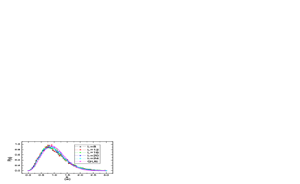
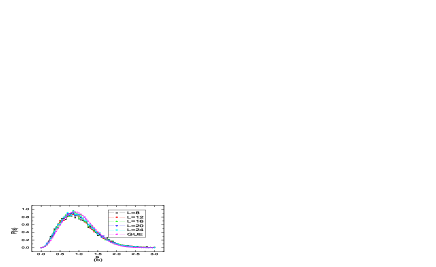
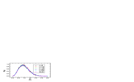
Figure 5: $P(s)$ vs. $s$ for $L=8,12,16,20,24$ and comparison with the Gaussian unitary ensemble $P_{GUE}(s)$. (a) $E=0$ and $P=0.1$; (b) $E=0.02$ and $P=0.1$; (c) $E=0.5$ and $P=1.5$.

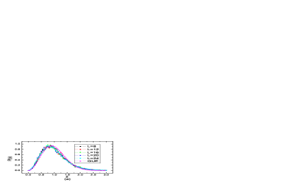
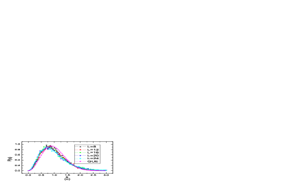
Figure 6: $P(s)$ vs. $s$ for $L=8,12,16,20,24$ and comparison with the Gaussian unitary ensemble $P_{GUE}(s)$. (a) $E=0$ and $P=0.7$; (b) $E=0.02$ and $P=0.7$; (c) $E=0.5$ and $P=0.5$.

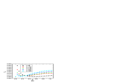
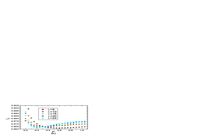
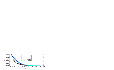
Figure 7: $I_{0}$ vs. $P$ for $L=8,12,16,20,24$, (a) $E=0$; (b) $E=0.02$; (c) $E=0.5$.

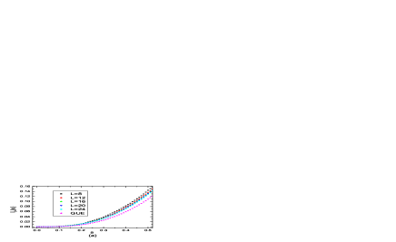
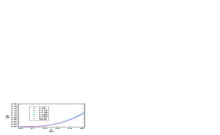
Figure 8: $I_{P}(s)$ vs. $s$ for $L=8,12,16,20,24$ and comparison with that of $P_{GUE}(s)$. (a) $E=0$ and $P=0.1$; (b) $E=0.02$ and $P=0.1$; (c) $E=0.5$ and $P=1.5$.

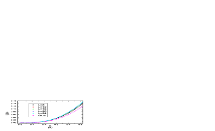
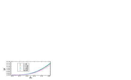
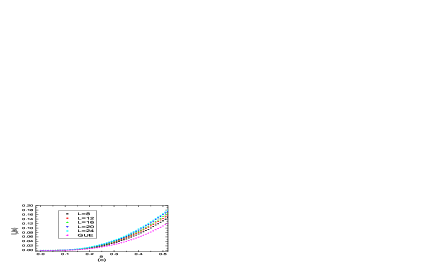
Figure 9: $I_{P}(s)$ vs. $s$ for $L=8,12,16,20,24$ and comparison with that of $P_{GUE}(s)$, (a) $E=0$ and $P=0.7$; (b) $E=0.02$ and $P=0.7$; (c) $E=0.5$ and $P=0.5$.

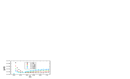
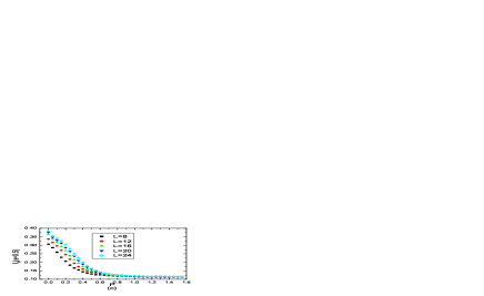
Figure 10: $I_{P}(s=0.5,P)$ vs. $P$ for $L=8,12,16,20,24$, (a) $E=0$; (b) $E=0.02$; (c) $E=0.5$.

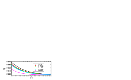
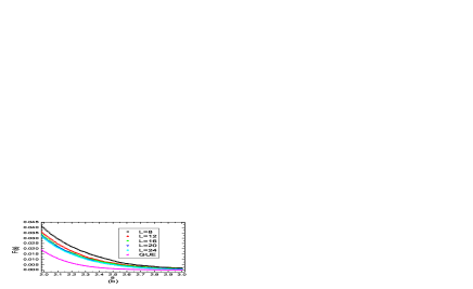
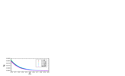
Figure 11: $F(s)$ vs. $s$ for $L=8,12,16,20,24$, and comparison with that of $P_{GUE}(s)$. (a) $E=0$ and $P=0.1$; (b) $E=0.02$ and $P=0.1$; (c) $E=0.5$ and $P=1.5$.

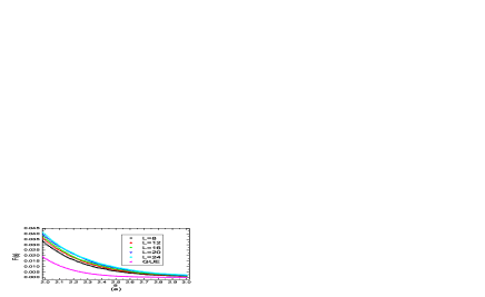
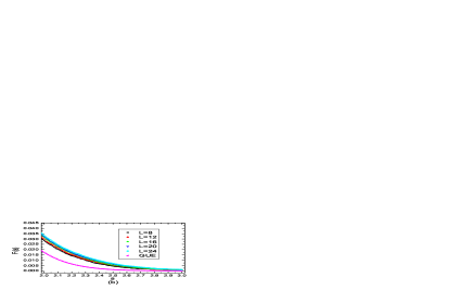
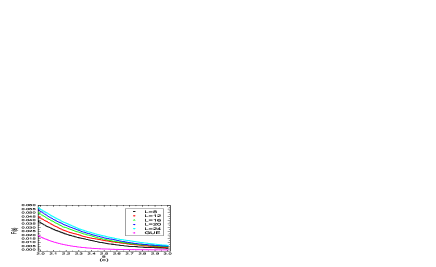
Figure 12: $F(s)$ vs. $s$ for $L=8,12,16,20,24$ and comparison with that of $P_{GUE}(s)$. (a) $E=0$ and $P=0.7$; (b) $E=0.02$ and $P=0.7$; (c) $E=0.5$ and $P=0.5$.

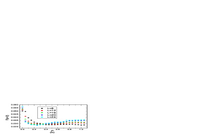
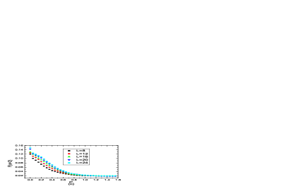
Figure 13: $F(s=2,P)$ vs. $P$ for $L=8,12,16,20,24$, (a) $E=0$; (b) $E=0.02$; (c) $E=0.5$.

The global shape of these curves has some common features. All curves have a vanishing value when $s$ tends to zero. At small $s$ they increase with $s$ and reach a peak at some intermediate $s$. Then they decrease with increasing $s$ and tend to vanish at large $s$. All these features are the same as the GUE distribution $P_{GUE}(s)$metzler . Thus most of them are close to $P_{GUE}(s)$ at first glance. This raises the question on how to distinguish between extended states and localized states by our numerical results. As a simple way, it is natural to expect that $P(s)$ of extended states should tend closer to $P_{GUE}(s)$ or remain unchanged with increasing $L$ while that of localized states should deviate from $P_{GUE}(s)$ with increasing $L$. By careful observation one can indeed see that curves in each sub-figure of Fig.5 tend to be closer to $P_{GUE}(s)$ with increasing $L$ while those in Fig.6 show the opposite tendency. Thus we can use the different tendency of $P(s)$ with increasing $L$ to distinguish between extended states and localized states. In the following, we shall show quantitatively such opposite tendencies for extended states and localized states by considering several characteristic quantities of $P(s)$.

Let us first consider a characteristic quantity $I_{0}$ defined by $I_{0}=\int s^{2}P(s)ds/2$. It is commonly used to characterize the global shape of $P(s)$ and to exam the localization propertymetzler . It is well-known that $I_{0}=1$ for localized states while $I_{0}<1$ for extended statesmehta . Thus, the following simple criteria is employed. If $I_{0}$ of a state with energy $E$ increases and approaches $1$ with increasing $L$, this state is localized. Otherwise, it is extended. Curves in Fig.7 are $I_{0}$ vs. mixing strength $P$ at $E=0$ (a); 0.02 (b); and 0.5 (c) for $L=8,12,16,20,24$. Fig.7(a) shows that the state at $E=0.02$ is localized at zero mixing and extended at small $P$. Then it is localized again after $P$ passes a particular $P_{c}$ where $I_{0}$ of different $L$ cross. For the state at the lower band center $E=0$ shown in Fig.7(b), it is extended at zero mixing. Then, it shows the same feature as the state of $E=0.02$ at small and large $P$. Fig.7(c) shows that state at $E=0.5$ is always localized at small $P$ and extended only for large $P(>1)$ where all curves of different system sizes tend to merge together.

It is well-known that a fundamental difference between $P(s)$ of localized and extended states is its behavior at small $s$. When $s$ tends to zero, $P(s)$ tends to zero for extended states due to level-repulsion while for localized states it tends to one due to level-aggregationmehta . Thus we need to consider the behavior of $P(s)$ at small $s$ for further test of the results in the last paragraph. It is convenient to consider a function of integrated level-spacing distribution at small $s$ defined by $I_{P}(s)=\int_{0}^{s}P(s^{\prime})ds^{\prime}$. The meaning of $I_{P}(s)$ is the integrated fraction of level-spacings smaller than $s$. Although $P(s)$ in most cases of our numerical results is close to the GUE distribution, level-repulsion of extended states and level-aggregation of localized states should still be expected at small $s$. This leads to the following criteria for localization property : $I_{P}(s)$ at small $s$ should increase with increasing $L$ for localized states while decrease or remain unchanged with increasing $L$ for extended states. Thus the behavior of $I_{P}(s)$ at small $s$ can serve as another method to distinguish between extended and localized states. Fig.8 shows $I_{P}(s)$ for $(E=0,P=0.1)$ (a), $(E=0.02,P=0.1)$ (b) and $(E=0.5,P=1.5)$ (c) for $L=8,12,16,20,24$ and comparison with $I_{P}(s)$ of $P_{GUE}(s)$. Fig.9 is for $(E=0,P=0.7)$ (a), $(E=0.02,P=0.7)$ (b) and $(E=0.5,P=0.5)$ (c). One can see clearly that states in Fig.8 show the feature of extended states while states in Fig.9 are localized. In order to exam each electronic state of fixed electronic energy $E$ in the whole range of mixing, we consider $I_{P}(s=0.5)$, the fraction of the level-spacings less than $0.5$. We plot the results of $I_{P}(s=0.5)$ vs. $P$ at $E=0,0.02$ and $0.5$ for L=8, 12, 16, 20, 24 in Fig.10. Similar with the criteria for $I_{P}(s)$, we use the following criteria. If $I_{P}(0.5)$ of a state increases with increasing $L$, the state is localized. Otherwise, they are extended. According to this criteria, curves in Fig.10 lead to essentially the same results for localization property as obtained by the analysis of $I_{0}$ in Fig.7, consistent with the results in the last paragraph.

Let us now turn to the region of large $s$. Since $P_{GUE}(s)$ decays faster than $P_{PE}(s)$ at large $s$, the behavior of $P(s)$ in this region can also be used to show difference between extended states and localized states. At this region it is convenient to consider another function of integrated level-spacing distribution defined by $F(s)=\int_{s}^{\infty}P(s)ds=1-I_{P}(s)$. The meaning of $F(s)$ is the integrated fraction of level-spacings larger than $s$. Since $F(s)$ of $P_{GUE}(s)$ is less than that of $P_{PE}(s)$ at large $s$, we may expect that $F(s)$ at larger $s$ decreases or remains unchanged with increasing $L$ for extended states while it increases with increasing $L$ for localized states. Fig.11 shows curves of $F(s)$ at $(E=0,P=0.1)$ (a), $(E=0.02,P=0.1)$ (b), and $(E=0.5,P=1.5)$ (c) for $L=8,12,16,20,24$ and comparison with that of $P_{GUE}(s)$. Fig.12 shows $(E=0,P=0.7)$ (a), $(E=0.02,P=0.7)$ (b), and $(E=0.5,P=0.5)$ (c). In view of Fig.8 and Fig.9, it is clear that the results of $F(s)$ coincide with those of $I_{P}(s)$ concerning the localization property. We also calculate $F(s=2)$ for each fixed energy in the whole range of mixing. As shown above, the same criteria as that for $I_{0}$ and $I_{P}(s=0.5)$ can be employed. The curves of $F(s=2)$ vs. $P$ are plotted in Fig.13 for $E=0$ (a), $E=0.02$ (b) and $E=0.5$ (c). One can see that they are consistent with the results of $I_{0}$ (Fig.7) and $I_{P}(s=0.5)$ (Fig.10).

IV.2 Discussion of the localization property

In the last subsection, we analyzed the global shape of $P(s)$ and its behavior at small and large $s$ by considering $I_{0}$, $I_{P}(s)$ and $F(s)$, respectively. Analysis of all these quantities leads to essentially the same conclusion concerning the localization property, as follows. For zero interband mixing, only states at the two LB centers are extended. In the presence of interband mixing, new extended states emerge. States near the LB centers,— i.e., $E\sim 0$,— are delocalized by weak interband mixing and localized by strong mixing, with a transition point at some intermediate mixing $P_{c}$. For states near the region between two LBs,—i.e., $E\sim 0.5$,— they are localized at both weak and intermediate mixing and delocalized by strong mixing.

The existence of new extended states at $E\sim 0.5$ in the case of strong interband mixing can be understood as follows. Assume that the intra-band tunneling at nodes are negligibly weak for states of $E\sim 0.5$, we saw already from Fig. 3(a) that the maximum interband mixing ($\sin\theta=1$) delocalizes the state, which is localized at zero interband mixing. If one views $p=\sin^{2}\theta$ as connection probability of two neighboring loops of opposite chirality, our two-channel model without intra-band tunnelings at nodes is analogous to a bond-percolation problem. It is well-known that a percolation cluster exists at $p\geq p_{c}=1/2$ or $P\geq P_{c}=1$ for a square latticestauff . Therefore, an extended state is formed by strong mixing. One hopes that the intra-band tunnelings at nodes will only modify the threshold value of the mixing strength.

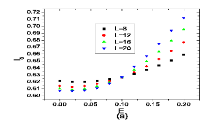
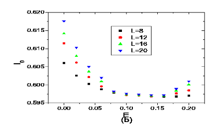
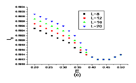
Figure 14: $I_{0}$ vs. $E$ for $L=8,12,16,20$, (a) $P=0.1$; (b) $P=0.7$; (c) $P=1.5$.

In order to show explicitly the existence of a narrow band of extended states and its evolution with increasing mixing, curves of $I_{0}$ vs. $E$ are plotted for three values of $P$ in Fig.14. A band of extended states is formed around the LB center $E\in[0,0.1]$ for $P=0.1$. When $P$ is increased to an intermediate value $0.7$, this band of extended states is lifted up to $E\in[0.8,1.6]$. For strong mixing, it is further shifted to $E\in[0.4,0.5]$. Thus the band of extended states in the lower LB emerges in weak mixing and tends to float up in energy with increased mixing. By symmetry one can expect that the extended band of the upper LB should tend to dive down in energy with increased mixing. The two bands of extended states in the lower and upper LBs should finally meet at the middle energy region in the case of strong mixing.

The above results are restricted to the case of two LBs, while there can be infinite LBs in the continuum model for a realistic system. Combine our above results and the float-up-merge picture proposed by Sheng et. al.sheng2 , one can expect the following conclusions for multiple LBs. In the case of weak interband mixing, a narrow extended band emerges in each LB. With increasing mixing, i.e., increasing disorders or decreasing magnetic field, the extended band in the lowest LB floats up and finally merges with that in the second lowest LB. Then, this extended band will further shift up and merge into that in the third lowest LB, and so on so forth.

To express our numerical results in the plane of energy and interband mixing, a topological phase diagram shown in Fig. 15(a) is obtained. In the absence of interband mixing, only the singular energy level at each LB center is extended. In the presence of interband mixing of opposite chirality, there are two regimes. At weak mixing, each of the extended states broadens into a narrow band of extended states near the LB centers. With increased mixing, the extended states in the lowest LB shift from the LB center(see Fig.14). These extended states will eventually merge with those from the higher LBs. This shifting of extended states was also observed beforekivelson . At strong mixing, a band of extended states exists between neighboring LBs where all states are localized without the mixing.

Let us look at the consequences of the above results. For weak disordered systems in IQHE regime, the Landau gap is larger than the LB bandwidth. Thus there is no overlap between adjacent LBs. According to the semiclassical picture, electronic states between the two adjacent LBs should be from either the upper or the lower bands with the same chirality in this case. It means that no interband mixing occurs and there is only one extended state in each LB. This may explain why scaling behaviors were observed for plateau transitions in early experiments on clean samples. Interband mixings occur when the Landau gap is less than the LB bandwidth. Systems of relatively strong disorders in IQHE regime should correspond to this case. As the single extended state at each LB center broadens into a narrow extended band, a narrow metallic phase emerges between two neighboring IQHE phases. Thus each plateau transition contains two consecutive quantum phase transitions for strongly disordered systems. The bands of extended states will merge together in strong mixing. This strong mixing regime corresponds to the case when the Landau gap is much smaller than the bandwidth. Since the Landau gap is proportional to the magnetic field, the disordered system should always enter the strong mixing regime before it reaches the weak field insulating phase, regardless of how weak the disorders are. In terms of QH plateau transitions, a direct transition occurs because a narrow metallic phase exists between two QH phases in a weak field. Thus, we propose that a direct transition from an IQHE phase to the insulating phase at weak field is realized by passing through a metallic phase, and it should hold for both weak and strong disordered systems.

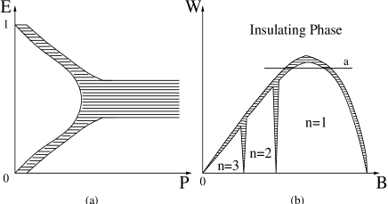
Figure 15: (a) Topological phase diagram of electron localization in $E-P$ plane. The shadowed regime is for extended states (metallic phase). (b) Topological QH phase diagram in $W-B$ plane. $W$ stands for the disorder strength, and $B$ for the magnetic field. The shadowed regime is for the metallic phase. The area indicated by the symbol $n$ is the $n$-plateau IQHE phase. The rest area is the insulating phase.

Plot above results in the plane of disorder and the magnetic field, we obtain a new topological QH phase diagram as shown in Fig. 15(b). This is similar to the empirical diagram obtained experimentally in Ref. 14. The origin ($W=0,\ B=0$) is a singular point. According to the weak localization theoryabrahams , no extended state exists at this point. Differing from existing theories, there exists a narrow metallic phase between two adjacent IQHE phases and between an IQHE phase and an insulating phase. This new phase diagram is consistent with the non-scaling experimentshilke where samples are relatively dirty, and interband mixing is strong, corresponding to a process along line $a$ in Fig. 15(b). The system undergoes two quantum phase transitions each time it moves from the QH insulating phase to IQHE phase of $n=1$ and back to the weak field insulating phase as the magnetic field decreases.

Figure 16: Experiment data of the logarithm of the longitudinal resistance $\ln[R_{xx}(f,T)/R_{xx}(0.647,40mK)]$ in Ref. 17. $f$ is the filling factor of LBs and $T$ is the temperature.

To verify this claim, we analyzed the original experimental data in Ref. 17 according to the assumption of two quantum phase transition points. The experiment data of the logarithm of the longitudinal resistance $ln[R_{xx}(f,T)]$ are shown in Fig. 16 where $f$ is the filling factor of LBs and $T$ is the temperature. According to the theory of continuous transitions, one should obtain

$$ln[R_{xx}(\nu,T)]=F_{1}(S_{1}(f)/T)$$ (12)

with $S_{1}(\nu)\sim(f_{c1}-f)^{z_{1}\nu_{1}}$ for the region of $f<f_{c1}$ while

$$ln[R_{xx}(\nu,T)]=F_{2}(S_{2}(f)/T)$$ (13)

with $S_{2}(\nu)\sim(f-f_{c2})^{z_{2}\nu_{2}}$ for the region of $f>f_{c2}$. Previous theories predict one single critical point, —i.e., $f_{c1}=f_{c2}$ and $z_{1}\nu_{1}=z_{2}\nu_{2}$. But our results suggest two distinct critical points. By standard scaling analysis, two good scaling behaviors are obtained for two close critical filling factors of $f_{c1}=0.6453$ and $f_{c2}=0.6477$ as shown in Fig. 17. The critical exponents in both the left side and the right side of the transition region are equal to the value $z\nu=2.33\pm 0.01$. On the other hand, the fit for one single critical point fails. Fig. 18 shows the result of a single critical point at $\nu_{c}=0.646$. It is the best fitting result for a single critical point if we require that the two critical exponents are approximately equal and the scaling law is optimally obeyed. The two critical exponents are $z_{1}\nu_{1}=2.58\pm 0.02$ and $z_{2}\nu_{2}=2.60\pm 0.02$, deviating from the theoretical results $\nu\sim 2.33$. One can also see clearly systematic deviations from the scaling law in the region close to the critical point at both sides in Fig. 18. This implies that the transition process is governed by two separated critical points instead of one. The regime between the two critical points should correspond to the metallic phase. Our fitting shows that the width of this regime is about $5\times 10^{-3}tesla$ while the value of the magnetic field was increased by $1\sim 2\times 10^{-3}tesla$ each time in the experiments. This may explain why the metallic phase was overlooked.

Figure 17: The fitting result of two critical points at the left and the right side. The two straight lines show coincidence with the scaling law. The critical filling factors are $f_{c1}=0.6453$ and $f_{c2}=0.6477$. The two critical exponents are equal to the value $z\nu=2.33\pm 0.01$.

Figure 18: The best fitting result of one single critical point at the left and right side. The critical filling factor is $f_{c}=0.646$. The two straight lines illustrate systematic deviations from the scaling law at regions close to the critical point. The average values of the two critical exponents are $z_{1}\nu_{1}=2.58\pm 0.02$ and $z_{2}\nu_{2}=2.60\pm 0.02$, respectively.

It is worth noting that there is another puzzle in the non-scaling experiment which may be solved by our two-critical-point picture. To be specific, let us consider the experimental data for the transition between the QH insulating phase and the $n=1$ IQHE phase. It was shown that the logarithm of the longitudinal resistance $ln[R_{xx}(f,T)]$ can be fitted with a linear function of the LB filling factor $f$ (see Fig.16) as followinghilke

$$ln[R_{xx}(f,T)]=ln[R_{xx}(f_{c},T)]-(f-f_{c})/(\alpha+\beta T)]$$ (14)

where $\alpha$ and $\beta$ are positive constants, $f_{c}$ is the filling factor where curves of different temperature $T$ cross approximately. Since $\alpha$ is non-zerohilke , it leads to the conclusion that $R_{xx}(f,T)$ at the limit of $T=0$ remains finite for every $f$. This is puzzling because it is inconsistent with the theoretical requirement that $R_{xx}(T=0)=\infty$ in the QH insulating phase, i.e., $f<f_{c}$, and $R_{xx}(T=0)=0$ in the $n=1$ IQHE phase, i.e., $f>f_{c}$. This puzzle may be solved as follows. Combine the linear relationship between $ln[R_{xx}(f,T)]$ and $f$ for fixed $T$ with our picture of two critical points $f_{c1}<f_{c2}$, we expect

$$ln[R_{xx}(f,T)]=ln[R_{xx}(f_{c1},T)]-(f-f_{c1})/(A_{1}T^{z\nu})$$ (15)

in the QH insulating phase, i.e., $f<f_{c1}$, while

$$ln[R_{xx}(f,T)]=ln[R_{xx}(f_{c2},T)]-(f-f_{c2})/(A_{2}T^{z\nu})$$ (16)

in the n=1 IQHE phase, i.e., $f>f_{c2}$, where $A_{1}$ and $A_{2}$ are positive constants, and $z$ and $\nu$ are critical exponents. It is clear that both $R_{xx}(f,T=0)=\infty$ in $f<f_{c1}$ and $R_{xx}(f,T=0)=0$ in $f>f_{c2}$ are recovered. While a finite value of $R_{xx}(f,T=0)$ in the region $f_{c1}<f<f_{c2}$ is consistent with our prediction of a metallic phase between the two critical points.

Our model can also be used to describe spin-polarized systems. In this case, the two LBs are for spin up and spin down states. Indeed, two-channel CC models have been used before to simulate a spin-resolved problemwang . In the presence of interband mixing, two distinct critical points were obtained. They were related to the two extended states in the two subbands, which are shifted by the mixings. However, this study could not discern whether the states in between are extended or localized. Thus it was not clear whether the extended states in the presence of mixing are just the two points or form a band. In this sense, our results are consistent with those of early works. It is worth noting that the spin resolved problem is different from the non-scaling experiment. In the spin resolved problem, the energy region considered includes the centers of both the spin-up and spin-down subbands. Thus there are two near-degenerate extended states in this region in the absence of interband mixing. It is then natural to regard the two distinct critical points as two distinct extended states of the two subbands in the presence of mixing. However, in the non-scaling experiment, the region considered includes only the center of the lowest LB. Thus there is only one extended state in the absence of interband mixing. In this case, the two separate critical points may not be considered as two distinct extended states. It seems that the only suitable explanation is the existence of a band of extended states between the two points.

One should also notice that two types of metallic phases have been studied extensively in the QH system. One is the composite Fermion state at the half-filling in the lowest Landau level (LL) and the other is the stripe state at the half-filled higher LLs. These states are formed by the Coulomb interaction effect in the high mobility samples. They are different from our metallic phase due to level mixing in the paper. Although we have not considered the electron-electron interactions in our study, there is no reason why the delocalization effect dof level mixing will be diminished by the Coulomb interaction. Of course, the interaction could change the level mixing effect’s dependence on the magnetic field.

V Conclusions

In conclusion, we find by numerical calculations within the network model that the single extended state at each LB center in the absence of interband mixing broadens into a narrow band of extended states when the effect of mixing of states of opposite chirality is taken into account. With the decrease of magnetic field or increase of disorders, these extended bands further broaden and may merge together. Based on this, we propose a new phase diagram in which a narrow metallic phase exists between two neighboring IQHE phases and between an IQHE phase and an insulating phase. This new phase diagram is consistent with non-scaling behaviors observed in recent experiments. A standard scaling analysis on experiment data in Ref. 17 supports our results.

*

Appendix A

Figure 19: A two-channel network model of $2\times 2$ nodes with periodic boundaries along both directions. $Z$’s are the wavefunction amplitudes on links. The notations are as follows. H and V stand for horizontal and vertical links, respectively. $u$ ($l$) is for the upper (lower) LB. $\hat{S}_{i}$ are SO(4) matrices describing tunneling at nodes, and $\hat{M}_{i}$ are $U(2)$ matrices for interband mixing.

In this appendix, we explicitly construct the evolution matrix $\hat{U}$ for a $2\times 2$ two-channel CC-network model as shown in Fig. 19. Periodical boundary conditions in both directions are imposed as explained in section III. $Z$-s are the wavefunction amplitudes on links. The notations are as follows. H and V stand for horizontal and vertical links, respectively. $u$ ($l$) is for the upper (lower) LB. $\hat{S}_{i}$ are SO(4) matrices defined in Eq. 3 describing the tunneling on nodes, and $\hat{M}_{i}$ are $U(2)$ matrices defined in Eqs. 5 and 6 describing interband mixing. From Fig. 19 we can obtain

$$\left(\begin{array}[]{l}Z_{u,H}^{1}(t+1)\\ Z_{l,H}^{1}(t+1)\\ Z_{l,H}^{2}(t+1)\\ Z_{u,H}^{2}(t+1)\end{array}\right)=\hat{H}_{1}\left(\begin{array}[]{l}Z_{l,V}^{1}(t)\\ Z_{u,V}^{1}(t)\\ Z_{u,V}^{2}(t)\\ Z_{l,V}^{2}(t)\end{array}\right)$$ (17)

$$\left(\begin{array}[]{l}Z_{u,H}^{3}(t+1)\\ Z_{l,H}^{3}(t+1)\\ Z_{l,H}^{4}(t+1)\\ Z_{u,H}^{4}(t+1)\end{array}\right)=\hat{H}_{2}\left(\begin{array}[]{l}Z_{l,V}^{3}(t)\\ Z_{u,V}^{3}(t)\\ Z_{u,V}^{4}(t)\\ Z_{l,V}^{4}(t)\end{array}\right)$$ (18)

$$\left(\begin{array}[]{l}Z_{l,V}^{1}(t+1)\\ Z_{u,V}^{1}(t+1)\\ Z_{u,V}^{2}(t+1)\\ Z_{l,V}^{2}(t+1)\end{array}\right)=\hat{H}_{3}\left(\begin{array}[]{l}Z_{u,H}^{3}(t)\\ Z_{l,H}^{3}(t)\\ Z_{l,H}^{4}(t)\\ Z_{u,H}^{4}(t)\end{array}\right)$$ (19)

$$\left(\begin{array}[]{l}Z_{l,V}^{3}(t+1)\\ Z_{u,V}^{3}(t+1)\\ Z_{u,V}^{4}(t+1)\\ Z_{l,V}^{4}(t+1)\end{array}\right)=\hat{H}_{4}\left(\begin{array}[]{l}Z_{u,H}^{1}(t)\\ Z_{v,H}^{1}(t)\\ Z_{l,H}^{2}(t)\\ Z_{u,H}^{2}(t)\end{array}\right),$$ (20)

with

$$\hat{H}_{1}=\left(\begin{array}[]{ll}\hat{1}&\hat{0}\\ \hat{0}&\hat{M}_{1}\end{array}\right)\hat{S}_{1};\quad\hat{H}_{2}=\left(\begin{array}[]{ll}\hat{M}_{2}&\hat{0}\\ \hat{0}&\hat{1}\end{array}\right)\hat{S}_{2};$$

$$\hat{H}_{3}=\left(\begin{array}[]{ll}\hat{1}&\hat{0}\\ \hat{0}&\hat{M}_{3}\end{array}\right)\hat{S}_{3};\quad\hat{H}_{4}=\left(\begin{array}[]{ll}\hat{M}_{4}&\hat{0}\\ \hat{0}&\hat{1}\end{array}\right)\hat{S}_{4},$$

where $\hat{1}$ and $\hat{0}$ are the $2\times 2$ identity and zero matrices, respectively. If we define

$$\phi_{H}=\left(\begin{array}[]{l}Z_{u,H}^{1}\\ Z_{l,H}^{1}\\ Z_{l,H}^{2}\\ Z_{u,H}^{2}\\ Z_{u,H}^{3}\\ Z_{l,H}^{3}\\ Z_{l,H}^{4}\\ Z_{u,H}^{4}\\ \end{array}\right);\quad\phi_{V}=\left(\begin{array}[]{l}Z_{l,V}^{1}\\ Z_{u,V}^{1}\\ Z_{u,V}^{2}\\ Z_{l,V}^{2}\\ Z_{l,V}^{3}\\ Z_{u,V}^{3}\\ Z_{u,V}^{4}\\ Z_{l,V}^{4}\\ \end{array}\right),$$ (37)

then the evolution equation is

$$\left(\begin{array}[]{l}\phi_{H}(t+1)\\ \phi_{V}(t+1)\end{array}\right)=\hat{U}\left(\begin{array}[]{l}\phi_{H}(t)\\ \phi_{V}(t)\end{array}\right).$$ (38)

The evolution operator $\hat{U}$ is

$$\hat{U}=\left(\begin{array}[]{llll}\hat{0}&\hat{0}&\hat{0}&\hat{H}_{1}\\ \hat{0}&\hat{0}&\hat{H}_{2}&\hat{0}\\ \hat{H}_{3}&\hat{0}&\hat{0}&\hat{0}\\ \hat{0}&\hat{H}_{4}&\hat{0}&\hat{0}\end{array}\right),$$ (39)

where $\hat{0}$ is the $4\times 4$ zero matrix. It has the structure of Eq. 9.

References

- (1) E. Abrahams, P. W. Anderson, D. C. Licciardello, and T. V. Ramakrishnan, Phys. Rev. Lett. 42, 673 (1979).
- (2) A. M. M. Pruisken, in ‘The Quantum Hall Effect’, ed. by R. E. Prange and S. M. Girvin (Springer Verlag, New York, 1987).
- (3) H. P. Wei, D. C. Tsui, M. P. Paalanen, and A. M. M. Pruisken, Phy. Rev. Lett. 61, 1294 (1988).
- (4) S. Kivelson, D. H. Lee and S. C. Zhang, Phys. Rev. B 46, 2223 (1992).
- (5) D.Z. Liu, X.C. Xie, and Q. Niu, Phys. Rev. Lett. 76, 975 (1996); X.C. Xie, et al., Phys. Rev. B54, 4966 (1996).
- (6) Z. Q. Wang, D. H. Lee and X. G. Wen, Phys. Rev. Lett 72, 2454 (1994)
- (7) K. Yang and R. N. Bhatt, Phys. Rev. Lett. 76, 1316 (1996).
- (8) A. G. Galstyan and M. E. Raikh, Phys. Rev. B56, 1422 (1997).
- (9) D. N. Sheng and Z. Y. Weng, Phys. Rev. Lett. 78, 318 (1997); ibid 80, 580 (1998).
- (10) D. N. Sheng, Z. Y. Weng, and X. G. Wen, cond-mat/0003117.
- (11) F.D.M. Haldane and K. Yang, Phys. Rev. Lett. 78, 298 (1997).
- (12) H. W. Jiang et al., Phys. Rev. Lett. 71, 1439 (1993).
- (13) T. K. Wang et al., Phys. Rev. Lett. 72, 709 (1994).
- (14) I. Glozman, C. E. Johnson, and H. W. Jiang, Phys. Rev. Lett. 74, 594 (1995).
- (15) S. V. Kravchenko, W. E. Mason, J. E. Fureaux, V. M. Pudalov, Phys. Rev. Lett. 75, 910 (1995).
- (16) S.-H. Song, D. Shahar, D. C. Tsui, Y. H. Xie, Don Monroe, Phys. Rev. Lett. 78, 2200 (1997).
- (17) X. R. Wang, X. C. Xie, Q. Niu, and J. Jain, cond-mat/0008411.
- (18) M. Hilke, D. Shahar, S. H. Song, D. C. Tsui, Y. H. Xie and D. Monroe, Phy. Rev. B56, 15545 (1997); D. Shahar, M. Hilke, C. C. Li, D. C. Tsui, S. L. Sondhi, J. E. Cunningham and M. Razeghi, Solid State Commun. 107, 19 (1998).
- (19) D. E. Khmelnitskii, Phys. Lett. 106A, 182 (1984).
- (20) R. B. Laughlin, Phys. Rev. Lett. 52, 2304 (1984).
- (21) G. Xiong, S.D. Wang, Q. Niu, D.C. Tian, and X. R. Wang, Phys. Rev. Lett., 87, 216802 (2001).
- (22) J. T. Chalker and P. D. Coddington, J.Phys. C: Solid State Phys.21, 2665 (1988).
- (23) D. Stauff and A. Aharony, ‘Introduction to Percolation Theory’ (Taylor and Francis, London, 1994).
- (24) D. K. K. Lee and J. T. Chalker, Phys. Rev. Lett 72, 1510 (1994).
- (25) V. Kagalovsky, B. Horovitz and Y. Avishiai, Phys. Rev. B55, 7761 (1997).
- (26) H. A. Fertig and B. I. Halperin, Phys. Rev. B36, 7969 (1987).
- (27) X. C. Xie, X. R. Wang, and D. Z. Liu, Phys. Rev. Lett. 80, 3563 (1998).
- (28) I. Kh. Zharekeshev and B. Kramer, Phys. Rev. Lett. 79, 717 (1997); H. Pttempa and L. Schweitzer, Ann. Phys.(Leipzig) 8, Spec. Issue, Si209 (1999); and references therein.
- (29) M. Batch and L. Schweitzer, cond-mat/9608148; Y. Ono, T. Ohtsuki and B. Kramer, J. Phys. Soc. Jpn. 65, 1734 (1996).
- (30) M. L. Mehta, ‘Random Matrices’ , 2nd ed. (Academic Press, 1991).
- (31) R. Klesse and M. Metzler, Phys. Rev. Lett. 79, 721 (1997).
- (32) H. A. Fertig, Phys. Rev. B38, 996 (1988).
- (33) M. Metzler and I. Varga, J. Phys. Soc. Jpn. 67, 1856 (1998).