Power Law Distributions of Offspring and Generation Numbers in Branching Models of Earthquake Triggering

Abstract

We consider a general stochastic branching process, which is relevant to earthquakes as well as to many other systems, and we study the distributions of the total number of offsprings (direct and indirect aftershocks in seismicity) and of the total number of generations before extinction. We apply our results to a branching model of triggered seismicity, the ETAS (epidemic-type aftershock sequence) model. The ETAS model assumes that each earthquake can trigger other earthquakes (“aftershocks”). An aftershock sequence results in this model from the cascade of aftershocks of each past earthquake. Due to the large fluctuations of the number of aftershocks triggered directly by any earthquake (“fertility”), there is a large variability of the total number of aftershocks from one sequence to another, for the same mainshock magnitude. We study the regime where the distribution of fertilities $\mu$ is characterized by a power law $\sim 1/\mu^{1+\gamma}$. For earthquakes, we expect such a power-distribution of fertilities with $\gamma=b/\alpha$ based on the Gutenberg-Richter magnitude distribution $\sim 10^{-bm}$ and on the increase $\sim 10^{\alpha m}$ of the number of aftershocks with the mainshock magnitude $m$. We derive the asymptotic distributions $p_{r}(r)$ and $p_{g}(g)$ of the total number $r$ of offsprings and of the total number $g$ of generations until extinction following a mainshock. In the regime $\gamma<2$ for which the distribution of fertilities has an infinite variance, we find $p_{r}(r)\sim 1/r^{1+{1\over\gamma}}$ and $p_{g}(g)\sim 1/g^{1+{1\over\gamma-1}}$. This should be compared with the distributions $p_{r}(r)\sim 1/r^{1+{1\over 2}}$ and $p_{g}(g)\sim 1/g^{1+{1}}$ obtained for standard branching processes with finite variance. These predictions are checked by numerical simulations. Our results apply directly to the ETAS model whose prefered values $\alpha=0.8$ and $b=1$ puts it in the regime where the distribution of fertilities has an infinite variance. More generally, our results apply to any stochastic branching process with a power-law distribution of offsprings per mother.

I Introduction

All large earthquakes are followed by an increase of seismic activity known as “aftershocks.” Aftershock sequences of small earthquakes are less obvious because the aftershock productivity is weaker, but can be clearly observed when stacking many sequences alpha . It is thus natural to assume that each earthquake can trigger its own aftershock sequence, and that observed aftershock sequences result from the cascade of direct aftershocks (triggered directly by the mainshock) and indirect aftershocks (triggered by a previous aftershock of the mainshock). This assumption is the basis of the Epidemic Type Aftershock Sequence model (ETAS) of seismicity Ogata88 ; Ogata99 ; KK81 ; KK87 ; helmsor1 , which describes earthquake triggering as a branching process. In addition, the ETAS model includes the Omori law decay $\sim 1/(t+c)^{p}$ of the number of direct aftershocks as a function of the time $t$ since the mainshock, where $c$ is a small constant and $p$ is an exponent close to but larger than 1. Previous works on this model have shown that the ETAS model provides a better fit to aftershock sequences than a single Omori law (no secondary aftershocks) GuoO97 and that a significant fraction of aftershocks, of the order of 80%, are secondary aftershocks Felzer1 ; Felzer2 . The ETAS model has been used in many studies KK81 ; Felzer1 to describe or predict the spatio-temporal distribution of seismicity and reproduces many properties of real seismicity, including a renormalization of the Omori exponent from the local Omori law (direct aftershocks) to the global Omori law (observed rate of aftershocks including secondary aftershocks) Ogata99 ; SorSor ; helmsor1 , Båth’s law Bathlawpap , a diffusion of aftershocks and realistic foreshock properties foreshockp ; Forexp . In this work, we present an analytical derivation of the distribution of the total number of aftershocks, summed over all generations of the cascade of aftershock triggering, and of the distribution of the total number of generations of aftershocks before extinction.

There are two well known statistical laws that describe the scale-invariance of earthquake physics with respect to magnitudes. First, the (complementary cumulative) Gutenberg-Richter (GR) distribution of earthquake magnitudes gives the probability

$$p_{m}(m)\sim 10^{-bm}$$ (1)

that an earthquake has magnitude equal to or larger than $m$. This magnitude distribution $p_{m}(m)$ is not dependent on the magnitude of the triggering earthquake, i.e., a large earthquake can be triggered by a smaller one alpha ; Forexp .

Second, the average number of aftershocks triggered directly by an earthquake of magnitude $m$ is found to increase with $m$ as

$$N_{m}=K~{}10^{\alpha m}$$ (2)

where $K$ is a numerical factor independent of the magnitude. The number of direct aftershocks cannot be measured, because what is observed is the total number of direct and secondary aftershocks. If earthquake triggering can be described by a branching process such as the ETAS model, then it can be shown that the scaling of the total number of aftershocks with the mainshock magnitude also obeys the law (2), but with a larger factor $K^{\prime}$ which accounts for the cascades of secondary aftershocks helmsor1 . The exponent $\alpha$ in (2) can thus be measured from a fit of the total number of aftershocks with the mainshock magnitude. Fits of the total number of aftershocks as a function of the mainshock magnitude in individual sequences support (2) with an exponent $\alpha$ in the range 0.75-1 6 ; 9 ; 11 ; 13 . However, the precision of these studies is limited by the narrow range of mainshock magnitudes considered and the large scatter of the number of aftershocks per mainshock. The value of $\alpha$ estimated in these studies may also be biased by the arbitrary constraint that aftershocks must be smaller than the mainshock, by the incompleteness of the catalog just after the mainshock, and by the background seismicity at large times after the mainshock. Other studies have measured the exponent $\alpha$ in (2) by calibrating the ETAS model to real data (individual aftershock sequences or complete catalogs) using maximum likelihood methods Ogata88 ; K91 ; GuoO97 ; Zhuangetal . These studies found a large scatter of the $\alpha$ exponent in the range $0.2-2$. It is not yet clear if this range of values reflects a real variability of $\alpha$ or the inaccuracy of the estimation of $\alpha$. One of us used a stacking method to estimate the average rate of earthquakes triggered (directly or indirectly) by a previous earthquake as a function of the magnitude of the triggering earthquake alpha , without constrain on the aftershock magnitude. For the catalog of the Southern California Data Center for Southern California, using the time period 1975-2003 and $m\geq 3$ earthquakes, $\alpha$ is found equal to $0.8\pm 0.1$, smaller than $b=1\pm 0.1$. Small earthquakes are thus collectively more important than larger earthquakes for earthquake triggering if $\alpha\leq b$, because they are much more numerous than larger ones.

Let us combine the two laws (1) and (2) to get the unconditional probability density for the number $N_{m}$ of events triggered directly by any event whose magnitude $m$ is drawn at random from the GR law. For this, we note that

$${\rm Pr}({\rm fertility}\geq N_{m})={\rm Pr}(K~{}10^{\alpha m}\geq N_{m})={\rm Pr}(m\geq{1\over\alpha}\log_{10}{N_{m}\over K})\sim 10^{-{b\over\alpha}\log_{10}{N_{m}\over K}}\sim{1\over N_{m}^{b/\alpha}},$$ (3)

where $Pr$ means “Probability”. The first equality makes use of (2) and the third equivalence makes use of (1). Hence, the probability density of the fertilities $N_{m}$, for a magnitude $m$ drawn at random in the GR law, is

$$p_{N_{m}}(N_{m})\sim{1\over{N_{m}}^{1+\gamma}}~{},$$ (4)

with $\gamma=b/\alpha$. Typically, $b=1$ and $\alpha\approx 0.8$ alpha leading to $\gamma\approx 1.25$. Because $\gamma<2$, the variance of the fertility, for an earthquake of arbitrary magnitude drawn from the GR law, is mathematically infinite (if we assume the absence of a roll-off in the GR distribution, see below).

Beyond earthquakes, a multitude of phenomena can also be described by branching processes with power-law distributions of fertility. Stochastic branching processes indeed describe well a multitude of phenomena Athreya ; Sankaranarayanan from chain reactions in nuclear and particle physics, material rupture, fragmentation and earthquake processes, critical percolation cluster sizes and population growth models, to population and biological dynamics, epidemics, economic and social cascades and so on. Branching processes are also of particular interest because deep connections have been established with critical phenomena Vere76 ; Vere77 . Epidemic transmission of diseases, and more generally transmission processes involving avalanches spreading on networks such as the World Wide Web, cellular metabolic network, ecological food webs, social networks, and so on exhibit such heavy-tail probability density functions (PDF) given by (5) below, as a consequence of the well-documented power law distribution of connectivities among nodes. Our results are thus relevant to systems in which the number of offsprings may be large due to long-range interactions, long-memory effects or large deviation processes. Goh et al. Goh actually derive results that overlap with ours in the context of avalanches in social networks.

In branching processes with a finite variance of the number of daughters per mothers, various quantities exhibit power law distributions with universal exponents at criticality (in statistical physics, the term “universal” refers to the independence of the critical exponents on the microscopic details of the physics). This includes the distributions of cluster sizes, of the number of generations before extinction and of durations which are mean field Athreya ; Sankaranarayanan (“mean field” refers to the branching approximation which leads to a lack of dependence on the space dimension). In the case of earthquakes and for other systems mentioned above, the distribution of fertilities has an infinite variance, leading to an anomalous scaling of offsprings and generation numbers. While the number of direct aftershocks per mainshock for a fixed mainshock magnitude has a finite variance, usually modeled by a Poisson distribution, the effect of multiple cascades of triggering and the variability of the fertility of each earthquake lead to a much larger power-law distribution for the total number of aftershocks summed over all generations. As a consequence, there are huge fluctuations of the total number of aftershocks from one sequence to another one, for the same mainshock magnitude.

The goal of this paper is to provide a general exact derivation of the distribution of the total aftershock productivity of any earthquake, summed over all generations of the cascade of aftershock triggering. We also derive the exact distribution of the total number of generations of aftershocks before extinction in the case of a power-law distribution of fertility relevant for earthquakes and for many other systems. Beyond earthquakes our results apply to any branching process with a power-law distribution of fertilities.

II Model and main results

We consider a general branching process in which each progenitor or mother is characterized by its average number $N_{m}\equiv\kappa\mu(m)$ of children (first generation offsprings), where $\mu(m)=10^{\alpha(m-m_{0})}$ is a mark associated with an earthquake of magnitude $m\geq m_{0}$, $\kappa$ is a constant factor and $m_{0}$ is the minimum magnitude of earthquakes capable of triggering other earthquakes. We note $\mu$ the mark of an earthquake which has an arbitrary magnitude $m$ drawn according to the GR law. According to (3), the mark $\mu$ is distributed according to

$$p_{\mu}(\mu)={\gamma\over\mu^{1+\gamma}}~{},~{}~{}~{}1\leq\mu<+\infty,~{}~{}~{}~{}~{}\gamma=b/\alpha~{}.$$ (5)

Note that $p_{\mu}(\mu)$ is normalized: $\int_{1}^{+\infty}d\mu~{}p_{\mu}(\mu)=1$. The relation $N_{m}\equiv\kappa\mu(m)$ together with (5) thus ensures that the fertility obeys the law (4). For a fixed $\gamma$, the coefficient $\kappa$ then controls the value of the average number $n$ of children of first generation per mother:

$$n=\langle N_{m}\rangle=\kappa\langle\mu\rangle=\kappa{\gamma\over\gamma-1}~{},$$ (6)

where the average $\langle N_{m}\rangle$ is taken over all mothers’ magnitudes drawn in the GR law. In the terminology of branching processes, $n$ is called the branching ratio. For $n<1$, there are less than one child per mother: this corresponds to transient (sub-critical) branching processes with finite lifetimes with probability one. For $n>1$, there are more than one child per mother: this corresponds to explosive (super-critical) branching processes with a number of events growing exponentially with time. The value $n=1$ of exactly one child per mother on average is the critical point separating the two regimes.

The realized number of children of an earthquake of fixed magnitude $m$ can be deterministic or may result from a Poisson or other more general distribution with mean $\kappa\mu(m)$. Any given child $i$ may then generate an average number $\kappa\mu_{i}$ of children, where the mark $\mu_{i}$ is specific to the child $i$ and is drawn from the PDF (5). These grand-children of the initial progenitor in turn generate new children with marks drawn from (5), and so on. The process cascades down along generations.

Here, we focus on global quantities $p_{r}(r)$ (total number $r$ of offsprings until extinction following a mainshock) and $p_{g}(g)$ (total number $g$ of generations until extinction following a mainshock). Therefore, arbitrary time-dependent branching processes can be considered and our results thus apply to arbitrary stochastic marked point-processes in discrete or continuous time. In particular, our results apply to the ETAS model. We have previously shown that, for $n<1$, the infinite variance of the number of first-generation events leads to anomalous global direct and inverse Omori law with apparent exponents varying continuously with $\gamma$ foreshockp . Our results also apply to variations of the ETAS models with different arbitrary time dependences.

In this work, we present an analytical derivation of the distribution of the total number of aftershocks, summed over all generations of the cascade of aftershock triggering, and of the distribution of the total number of generations of aftershocks before extinction. Specifically, we uncover a novel regime with continuously varying exponents for the probability density function (PDF) $p_{r}(r)$ of the total number $r$ of progenies and $p_{g}(g)$ of their total number $g$ of generations of aftershocks of a mainshock before extinction. This regime appears in the regime of large deviations $\gamma<2$ relevant for earthquakes, when the distribution of the number of first-generation offsprings from any mother has a power law tail with infinite variance.

We study the sub-critical and critical regimes for which the number $n$ of children per mother, averaged over all possible numbers of children per mother, is less than or equal to $1$. This condition $n\leq 1$ ensures that, with probability $1$, the cascade ends after a finite number of generations with a finite total number of offsprings Athreya ; Sankaranarayanan . Figure 1 presents comparisons between numerical simulations of branching processes for different values of $\gamma$ and our main result (at criticality $n=1$) derived below:

$$p_{r}(r)\approx C_{r}/r^{1+{1\over\gamma}}~{}~{};~{}~{}p_{g}(g)\approx C_{g}/g^{1+{1\over\gamma-1}}~{},$$ (7)

for $1<\gamma\leq 2$. $C_{r}$ and $C_{g}$ are two constants independent of $r$ and $g$, respectively, such that $p_{r}(r)$ and $p_{g}(g)$ are normalized to 1. For $n<1$, the intermediate asymptotics (7) holds for $r<R_{2}\simeq 1/(1-n)^{\gamma/(\gamma-1)}$ beyond which there is another power-law asymptotic

$$p_{r}(r)\sim 1/r^{1+\gamma}~{}.$$ (8)

For $\gamma\geq 2$ and $n=1$, the standard mean field scaling

$$p_{r}(r)\sim 1/r^{3/2}~{}~{}~{}~{}~{}~{}{\rm and}~{}~{}~{}~{}~{}~{}p_{g}(g)\sim 1/g^{2}$$ (9)

are retrieved. The regime $0<\gamma\leq 1$ gives rise to explosions and, in continuous time, to stochastic finite-time singularities sorhelmsing . If the GR law is truncated or exhibits a deviation from its standard form in the large magnitude range, our results will hold for intermediate values of $r$ and $g$ and will be truncated at large $r$’s and large $g$’s.

The following section gives the technical derivation of the results (7,8,9).

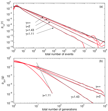
Figure 1: Numerical tests of the anomalous scalings (7) at criticality $n=\kappa\langle\mu\rangle=1$. The noisy lines are the Monte-Carlo simulations. The smoothed lines are the predictions (7). The deviation between theory and numerical simulations on $P_{g}(g)$ for $\gamma=1.1$ results from the very large theoretical exponent equal to $1+{1\over\gamma-1}=11$, describing a fast fall-off which is hard to document numerically since one decade in the horizontal scale corresponds to 11 decades on the vertical scale.

III General formulation

III.1 Formal solution in terms of Probability Generating Functions (PGF)

The most general relations of branching theory are expressed via probability generating functions (PGF) defined by

$$\langle z^{R}\rangle=\sum_{r=0}^{\infty}p_{r}(r)~{}z^{r}~{}$$ (10)

where $\langle\dots\rangle$ means statistical averaging. By definition, $p_{r}(r)=\text{Pr}(R=r)$ is the probability that the random variable $R$ takes the value $r$. It can be obtained from its PGF by the relation

$$p_{r}(r)=\text{Pr}(R=r)=\frac{1}{r!}\left.\frac{d^{r}\langle z^{R}\rangle}{dz^{r}}\right|_{z=0}\,.$$ (11)

The key property of PGFs is that the PGF of the sum of statistically independent summands is equal to the product of the summands PGF’s. This is useful for branching processes for which the number of daughters triggered by different mothers are statistically independent. We introduce four PGF’s: (i) $G_{\mu_{0}}(z)$ is the PGF of the number $R_{1}$ of daughters generated from a given mother with fertility $\kappa\mu$ at the first generation; (ii) $G(z)$ is the same as $G_{\mu}(z)$ but averaged over all mothers’ fertility $\kappa\mu$; (iii) $\Theta_{\mu}(z)$ is the PGF of the total number of daughters generated from a given mother with fertility $\kappa\mu$ summed over all generations; (iv) $\Theta(z)$ is the same as $\Theta_{\mu}(z)$ but for a mother of arbitrary fertility. Then, general branching theory Athreya ; Sankaranarayanan gives the functional equations

$$\Theta(z)=G(z\Theta(z))~{}~{}~{};~{}~{}~{}\Theta_{\mu}(z)=G_{\mu}(z\Theta(z))~{}.$$ (12)

Using $\langle R\rangle=d\Theta(z)/dz|_{z=1}$ and similarly for the other PGF, the formulas (12) lead to $\langle R\rangle=n/(1-n)$ for the number of daughters summed over all generations and averaged over all possible mother’s fertilities, where $n$ defined by (6) is the average number of first-generation daughters from mothers of arbitrary fertility.

Using Lagrange series, we transform the implicit equation (12) in $\Theta_{\mu}$ into an explicit equation. Recall that a Lagrange series is the Taylor expansion of the function $G_{\mu}(y(z,a))$ with respect to $z$, where $y(z,a)$ is solution of the implicit equation $y=a+z\,G(y)$. For infinitely differentiable functions $G_{\mu}(y)$ and $G(y)$ in the neighborhood of $z=a$, we have the following Taylor series

$$G_{\mu}(y)=G_{\mu}(a)+\sum_{k=1}^{\infty}\frac{z^{k}}{k!}\,\frac{d^{k-1}}{da^{k-1}}\left[G^{k}(a)\frac{dG_{\mu}(a)}{da}\right]\,.$$ (13)

In (12), we have $y(z,a=0)=z\,\Theta(z)$, and using the identity $p_{r,\mu}(r)=(1/r!)d^{r}\Theta_{\mu}(z)/dz^{r}|_{z=0}$ allowing to recover the PDF from its generating function, we obtain the explicit formula for the PDF $p_{r,\mu}(r)$ of the total number of daughters born from a mother with fertility $\mu$:

$$p_{r,\mu}(0) = G_{\mu}(0)$$ (14)

$$p_{r,\mu}(r) = \left.\,\frac{1}{r!}\,\frac{d^{r-1}}{dz^{r-1}}\left[G^{r}(z)\frac{dG_{\mu}(z)}{dz}\right]\right|_{z=0}~{},~{}~{}~{}~{}~{}r>0~{}.$$ (15)

Let us now specialize to the Poisson distribution

$$p_{r_{1},\mu}(r_{1})=\frac{(\mu\kappa)^{r_{1}}}{r_{1}!}\,e^{-\mu\kappa}~{},$$ (16)

giving the PDF of the number $R_{1}$ of daughters of first generation born from a mother with fertility $\mu$. By construction, the average of $R_{1}$ at fixed mother fertility $\mu$ over an ensemble of Poisson realizations is $\langle R_{1}\rangle_{\mu}=\mu\kappa$. The PGF associated with (16) is

$$G_{\mu}(z)=e^{\mu\kappa(z-1)}\,.$$ (17)

From (17), we obtain the expression of $G(z)$ by averaging over all possible fertilities $\mu$ according to the PDF (5). Using explicitly the normalized PDF $p_{\mu}(\mu)=\gamma/\mu^{1+\gamma}$ for $\mu\geq 1$ and $0$ otherwise, we obtain

$$G(z)=\gamma\,\kappa^{\gamma}(1-z)^{\gamma}\,\Gamma(-\gamma,\kappa(1-z))\,.$$ (18)

Expression (18) can be expanded as

$$G(z)\simeq 1-a_{1}~{}y~{}-~{}a_{\gamma}~{}y^{\gamma}~{}+~{}a_{2}~{}y^{2}~{}+~{}\dots$$ (19)

where $y=\kappa(1-z)$, $a_{1}=\frac{\gamma}{\gamma-1}$, $a_{\gamma}=\Gamma(1-\gamma)$ and $a_{2}=\frac{\gamma}{2(\gamma-2)}$. This expansion (19), valid for any $\gamma$, applies beyond the specific Poisson process (16). It is solely based on the asymptotic power law PDF (5) of the average number of daughters at the first generation. Thus, our asymptotic results (7) derived below hold under very general conditions.

III.2 Probabilistic interpretation

Let us provide a probabilistic interpretation of formula (15). In addition to be of intuitive appeal, it will be very useful for the derivation of our results.

Let us consider the random integer $R$ with PDF $P(k)=\text{Pr}(R=k)$ and its PGF as

$$S(z)=\sum_{k=0}^{\infty}P(k)z^{k}\,,$$ (20)

and reciprocally

$$P(k)=\text{Pr}(R=k)=\frac{1}{k!}\left.\frac{d^{k}S(z)}{dz^{k}}\right|_{z=0}\,.$$ (21)

Let us decompose $R=X+Y$, where $X$ and $Y$ are statistically independent random integers with PGFs $Q(z)$ and $G(z)$ respectively. Due to the statistical independence of $X$ and $Y$, we have $S(z)=Q(z)G(z)$ and relation (21) takes the form

$$P(k)=\text{Pr}(X+Y=k)=\frac{1}{k!}\left.\frac{d^{k}}{dz^{k}}\left[Q(z)G(z)\right]\right|_{z=0}\,.$$ (22)

Let in turn

$$Y=Y(r)=Y_{1}+Y_{2}+\dots+Y_{r}$$ (23)

where $\{Y_{1},\dots,Y_{r}\}$ are $r$ statistically independent random integers with the same PGF $G(z)$. Then, formula (22) takes the form

$$P(k)=\text{Pr}(X+Y(r)=k)=\frac{1}{k!}\left.\frac{d^{k}}{dz^{k}}\left[Q(z)G^{r}(z)\right]\right|_{z=0}\,.$$ (24)

Let us now rewrite relation (15) in a form similar to (24). For this, let us introduce the auxiliary PGF

$$Q_{\mu}(z)=\frac{1}{\left<r_{1}(\mu)\right>}\frac{dG_{\mu}(z)}{dz}\,.$$ (25)

It is easy to prove rigorously that, for an arbitrary PGF $G_{\mu}(z)$ possessing a finite mean value

$$\left<r_{1}(\mu)\right>=\left.\frac{dG_{\mu}(z)}{dz}\right|_{z=1}<\infty~{},$$ (26)

then the auxiliary function $Q_{\mu}(z)$ is indeed the PGF of some random variable. Moreover, in the case under consideration of a Poissonian PGF, we have

$$G_{\mu}(z)=e^{\mu\kappa(z-1)}\qquad\Rightarrow\qquad Q_{\mu}(z)\equiv G_{\mu}(z)=e^{\mu\kappa(z-1)}$$ (27)

and

$$\left<r_{1}(\mu)\right>=\mu\kappa\,.$$ (28)

One can thus rewrite relation (15) in the form

$$p_{r,\mu}(r)=\left.\,\frac{\mu\kappa}{r!}\,\frac{d^{r-1}}{dz^{r-1}}\left[G^{r}(z)G_{\mu}(z)\right]\right|_{z=0}\,.$$ (29)

Taking into account relation (24) and introducing the new random integer $X(\kappa\mu)$ possessing the Poissonian PGF (27), we can rewrite (29) in the form

$$p_{r,\mu}(r)=\frac{\mu\kappa}{r}\,\text{Pr}\left[X(\kappa\mu)+Y(r)=r-1\right]\,.$$ (30)

This is the key formula that we will use for deriving the asymptotic relations for the PDF $p_{r,\mu}(r)$ using limit theorems.

IV Distribution of the total number of aftershocks

IV.1 Case $\gamma\to\infty$

Let us first consider the limiting case $\gamma\to\infty$. The formal limit of a power law with an exponent going to infinity can be assimilated to an exponential in the following sense. Writing the tail of the complementary distribution as $A^{\gamma}/(A+\mu)^{\gamma}$, and assuming that $A$ also grows with $\gamma$ as $A=\gamma/a$, then $A^{\gamma}/(A+\mu)^{\gamma}=1/(1+a\mu/\gamma)^{\gamma}\to_{\gamma\to+\infty}\exp[-a\mu]$. This corresponds to an exponential tail for the distribution of the number of first generation daughters for arbitrary mother’s fertilities, as in (16) but with the same fertility for all mothers. In this case, $n=\kappa$ as can be seen from (6). This amounts to replacing expression (18) by $G(z)=e^{\kappa(z-1)}$ and we also have $G_{\mu}(z)=e^{\mu\kappa(z-1)}$. Thus,

$$G^{r}(z)\frac{dG_{\mu}(z)}{dz}=\mu\kappa\,e^{\kappa(z-1)(r+\mu)}~{}.$$

Correspondingly,

$$\frac{d^{r-1}}{dz^{r-1}}\left[G^{r}(z)\frac{dG_{\mu}(z)}{dz}\right]=\mu\kappa^{r}(r+\mu)^{r-1}\,e^{\kappa(z-1)(r+\mu)}~{}.$$ (31)

By substituting (31) into the right-hand-side of (15) gives exactly

$$p_{\mu}(r)=\mu\,\kappa^{r}~{}e^{-\kappa\mu}\,\frac{\left[(\mu+r)\,e^{-\kappa}\right]^{r}}{r!(\mu+r)}\,.$$ (32)

There are two ways of deriving asymptotic formulas for $p_{r,\mu}(r)$ in the case $\gamma=\infty$. The first one relies on Stirling’s formula $r!\simeq\sqrt{2\pi r}\,r^{r}e^{-r}$ applied to expression (32). The second method relies on the probabilistic interpretation of the general formula (15) given in section III.2 together with the central limit theorem. The formulas obtained by these two methods differ in details, but are actually very close quantitatively over the most part of the tail, and are easily checked to converge to the same result asymptotically. The approach using the Stirling formula works only for $\gamma=\infty$ and does not allow to derive more general results for $1<\gamma<\infty$. The second approach is much more powerful and elegant. In particular, all asymptotics and crossovers in the case $1<\gamma<\infty$ are obtained by the second approach.

Let us first examine the first method. Using the above mentioned Stirling’s formula, one can rewrite (32) in the form

$$p_{r,\mu}(r)=\frac{1}{\mu}\,f(x)\,\qquad x=\frac{r}{\mu}\,,$$ (33)

where

$$f(x)\simeq\frac{C}{\sqrt{2\pi x}~{}(1+x)}\left(1+\frac{1}{x}\right)^{\mu x}\,e^{-\mu\delta x}$$ (34)

and

$$C=\sqrt{\mu}\,e^{-\kappa\mu}\,,\qquad\delta=\kappa-\ln\kappa-1\,.$$ (35)

Because Stirling’s formula is very precise even for $r\simeq 1$ (for example $1!=1$ while Stirling’s formula gives $1!\simeq 0.922$, $2!=2$ while Stirling’s gives $2!\simeq 1.919$ and so on), formula (34) actually works well even for not too large $\mu$ and intermediate $\kappa<1$. The advantage of (34) is that it gives a clear understanding of the structure of the PDF $f(x)$. It consists of (i) a characteristic power tail

$$f(x)\propto\frac{1}{\sqrt{2\pi x}(1+x)}\sim x^{-3/2}\,,$$ (36)

(ii) an exponential decaying factor

$$f(x)\propto e^{-\mu\delta x}$$ (37)

which disappears when $\kappa=1$, i.e., $\delta=0$, and (iii) an algebraic factor

$$f(x)\propto\left(1+\frac{1}{x}\right)^{\mu x}\sim e^{\mu}\,\exp\left(-\frac{\mu}{x}\right)$$ (38)

which possesses a lower cut-off at $x\lesssim\mu$.

The shortcoming of (34) is that we can derive it only when an explicit expression such as (32) is available. We have not such luxury in the more general case $1<\gamma<\infty$ for which we need the second approach. Let us first quote the asymptotic formula (39) given below for $\gamma\to+\infty$ obtained from the application of the second probabilistic method. We shall show how to derive (39) as a special case of the next section for $2<\gamma$.

When the variance $\sigma_{1}^{2}$ of the number $r_{1}$ of daughters of the first generation from mothers of arbitrary fertilities is much greater than $1-\kappa$, we find (see next section) that, due to central limit theorem, expression (32) reduces to

$$p_{\mu}(r)\simeq\frac{\mu\kappa}{r\sqrt{2\pi\,\kappa\,(r+\mu)}}\,\exp\left(-\frac{[(1-\kappa)r-\mu\kappa-1]^{2}}{2\kappa\,(r+\mu)}\right)\,.$$ (39)

At criticality, $n=\kappa=1$, this expression becomes

$$p_{\mu}(r)\simeq\frac{\mu}{r\sqrt{2\pi r}}\,\exp\left(-\frac{\mu^{2}}{2r}\right)\,,$$ (40)

which retrieves the announced well-known mean field asymptotics $p_{\mu}(r)\sim 1/r^{3/2}$. The exponential term $\exp(-\mu^{2}/(2r))$ describes the roll-off of the number of aftershocks for small numbers close to the characteristic value $r\approx\mu^{2}$.

In the subcritical regime $n<1$, expression (32 ) gives an exponential decay of the number of aftershocks for large $r$.

These results can be checked explicitly as follows. The case of $\gamma\to+\infty$ corresponds either to $b\to\infty$ (all events have the same magnitude) or to $\alpha=0$ (all the events trigger the same expected number of offsprings independently of their magnitude). In both cases, $\mu$ tends to a constant independent of the mainshock magnitude. In order to check the above results, let us take this constant equal to $1$. This choice will modify the constants but not the functional dependences. Assuming $\mu=1$ transforms (32) into Taking $\mu=1$ transforms (32) into

$$p_{\mu}(r)=\kappa^{r}~{}{(r+1)^{r}\over(r+1)!}~{}e^{-\kappa(r+1)}~{}.$$ (41)

By using the Stirling formula, it has the approximation

$$p_{\mu}(r)\approx{e^{r\ln\kappa+(r+1)(1-\kappa)}\over\sqrt{2\pi}~{}(r+1)^{3/2}}~{}.$$ (42)

When $\kappa=n=1$ (critical case), we retrieve $p_{\mu}(r)\sim r^{-3/2}$. When $\kappa=n<1$ is close to $1$, $p_{\mu}(r)\sim r^{-3/2}~{}e^{-\delta~{}r}$ where $\delta$ is defined in (35).

IV.2 Case of finite variance $2<\gamma<\infty$

In this case, the summands in the sum (23) have a finite mean $\left<Y_{1}\right>$ and finite variance $\sigma^{2}_{1}$. Thus, the Central Limit Theorem (CLT) holds (see for instance Sorbook for a pedagogical exposition of the CLT). Let us recall the explicit expressions of the mean and variance:

$$\left<Y_{1}\right>=n=\frac{\kappa\gamma}{\gamma-1}\,,\qquad\sigma_{1}^{2}=\frac{n^{2}}{\gamma(\gamma-2)}+n\,,$$ (43)

If $r\gg 1$ (in practice, it is sufficient that $r\gtrsim 6$), the sum $Y(r)$ in (23) converges to a Gaussian variable with the following mean and variance

$$\left<Y(r)\right>=r\,n\,,\qquad\sigma^{2}(r)=r\sigma^{2}_{1}\,.$$ (44)

Let $\mu\kappa$ be integer (just for illustrative purpose). Then, one can imagine $X(\mu\kappa)$ as a sum

$$X(\mu\kappa)=\sum_{m=1}^{\mu\kappa}X_{m}$$ (45)

of independent summands $\{X_{1},X_{2},\dots,X_{\mu\kappa}\}$ with the following PGF, mean and variance:

$$Q(z)=e^{z-1}\,,\qquad\left<X_{1}\right>=\sigma^{2}=1\,.$$ (46)

If the number of summands $\mu\kappa\gg 1$, then the sum (45) is asymptotically Gaussian as well, with mean and variance equal to $\mu\kappa$.

Thus if $r\gg 1$ and $\mu\kappa\gg 1$, then the sum $X(\mu\kappa)+Y(r)$ is asymptotically Gaussian and we can use the following asymptotic formula

$$\text{Pr}\left[X(\kappa\mu)+Y(r)=m\right]=\frac{1}{\sqrt{2\pi\sigma_{\mu}^{2}(r)}}\exp\left[-\frac{(m-a_{\mu}(r))^{2}}{2\sigma_{\mu}^{2}(r)}\right]\,.$$ (47)

Here $a_{\mu}(r)$ and $\sigma_{\mu}^{2}(r)$ are respectively the mean and variance of the sum $X(\mu\kappa)+Y(r)$:

$$a_{\mu}(r)=rn+\mu\kappa\,,\qquad\sigma_{\mu}^{2}(r)=r\sigma_{1}^{2}+\mu\kappa\,.$$ (48)

Substituting (48) into (47) and (47) into (30), we obtain

$$p_{r,\mu}(r)\simeq\frac{\mu\kappa}{r\sqrt{2\pi(\sigma_{1}^{2}r+\mu\kappa)}}\,\exp\left(-\frac{[(1-n)r-\mu\kappa-1]^{2}}{2(\sigma_{1}^{2}r+\mu\kappa)}\right)\,.$$ (49)

For $\gamma=\infty$, for which we have the mean and variance defined in (43) reduce to $\sigma^{2}_{1}=n=\kappa$, relation (49) transforms into the previously announced result (39). In this case, we can test the quality of the general asymptotic relation (49) by comparing its particular application (39) with the exact expression (32) and its Stirling asymptotics (34). The exact and Stirling’s approximation essentially coincide while the “Gaussian” approximation is also excellent and goes closer and closer to the exact formula the larger $\mu$ is and the closer $n=\kappa$ is to $1$.

For $\sigma_{1}^{2}~{}r>\mu\kappa$, expression (49) can be simplified into

$$p_{\mu}(r)\simeq\frac{\mu\kappa}{r\sqrt{2\pi\sigma_{1}^{2}\,r}}\,\exp\left(-\frac{[(1-n)r-\mu\kappa-1]^{2}}{2\sigma_{1}^{2}\,r}\right)\,,$$ (50)

which reduces again to the standard mean field asymptotics (40) at the critical point $n=1$ and for $r\gg\mu^{2}\kappa^{2}$. Expression (50) is obtained using the following approximation

$$\sigma_{1}^{2}r+\mu\kappa\simeq\sigma_{1}^{2}r\,,$$ (51)

that is, by neglecting the term $\mu\kappa$. From a probabilistic point of view, this corresponds to using the Law of Large Numbers for the sum (45). Namely, if $\mu\kappa\gg 1$, then one can replace (45) by its mean field limit

$$X(\mu\kappa)\simeq\left<X(\mu\kappa)\right>=\mu\kappa~{},$$ (52)

which provides the truncated equality (51). Another reason for using the mean field limit (52) is more technical: in order to be able to effectively use the same technique in the case $1<\gamma<2$, we need to implement such a “mean field approximation.” Otherwise, the formulas would include very complicated convolutions of Gaussian and Levy stable laws.

We have checked the validity of the mean field approximation by comparing numerically the general asymptotics (49) and of its truncated mean field limit version (50) for various values of $\gamma$, $n$ and $\mu\kappa$. We find always an excellent convergence in the tail. For instance, consider the simplest case $\gamma=\infty$, for which the general asymptotic formula (49) transforms into (39), while its truncated mean field version is

$$p_{r,\mu}(r)\simeq\frac{\mu\kappa}{r\sqrt{2\pi\kappa r}}\,\exp\left(-\frac{[(1-\kappa)r-\mu\kappa-1]^{2}}{2\kappa r}\right)\,.$$ (53)

The agreement between all these expressions is excellent in the tails for all values of the parameters. The truncated mean field approximation describes satisfactory the body of distribution and becomes very precise in the tail of the distribution, even for moderate values of $\mu\approx 25$ and $n=\kappa<0.9$. Even better agreement is obtained for larger $\mu$ and closer to the critical case $n=1$.

Let us complement this section by a few additional useful formulas. The expansion (19) with $\langle r_{1}\rangle=dG(z)/dz|_{z=1}$ shows that the average number $r_{1}$ of first-generation daughters from mothers of arbitrary fertilities is $n=\langle\mu\rangle\kappa=\kappa\gamma/(\gamma-1)$ and that, for $1<\gamma<2$, the variance of $r_{1}$ is infinite. For $\gamma>2$, the variance of $r_{1}$ is $\sigma_{1}^{2}=n+n^{2}/[\gamma(\gamma-2)]$. The form of (19) is essentially controlled by the expression of the characteristic function of the PDF (5) and it is thus not a surprise that the PDF of the number of daughters of first generation born from a mother with arbitrary fertility has the same asymptotic form as (5). For a mother with fixed fertility $\mu$, the average and variance of the total number of daughters are respectively

$$\langle r_{\mu}\rangle=\frac{\mu\kappa}{1-n}~{}~{};~{}~{}\sigma^{2}_{\mu}=\frac{\mu\kappa}{(1-n)^{3}}\left[1+\frac{n^{2}}{\gamma(\gamma-2)}\right]~{},~{}~{}~{}~{}{\rm for}~{}~{}\gamma>2~{}.$$ (54)

IV.3 Case of infinite variance $1<\gamma<2$

We now turn to the novel regime $1<\gamma<2$. In this case, it is convenient to rewrite relation (15) in a more transparent probabilistic form

$$p_{\mu}(r)=\frac{\mu\kappa}{r}\,\text{Pr}\left[X+Y(r)=r-1\right]\,,Y(r)=\sum_{k=1}^{r}Y_{k}\,,$$ (55)

where $\{X,Y_{1},\dots,Y_{r}\}$ are mutually independent random integers such that the PGF of $X$ is $G_{\mu}(z)$ given by (17) while the PGF’s of the remaining integers are equal to $G(z)$ given by (18). For $1<\gamma<2$, the variance of each variable $Y_{k}$ is infinite, for the same reason that $\sigma_{1}^{2}$ is infinite. From the generalized limit theorem Major , $\tilde{Y}(r)=Y(r)-nr$ converges in distribution to a PDF $f_{y}(s)$ which is proportional to a stable infinitely-divisible PDF $\varphi_{\gamma}(x)$ with exponent $\gamma$

$$f_{y}(s)={1\over\nu r^{1/\gamma}}\varphi_{\gamma}\left({s\over\nu r^{1/\gamma}}\right)~{},$$ (56)

where

$$\nu=\kappa[\gamma\Gamma(-\gamma)]^{1/\gamma},$$ (57)

and

$$\varphi_{\gamma}(x)=\int\limits_{0}^{\infty}\exp\left(u^{\gamma}~{}\cos\left({\pi~{}\gamma\over 2}\right)\right)~{}\cos\left(u^{\gamma}~{}\sin({\pi~{}\gamma\over 2})+u~{}x\right)~{}du$$ (58)

with $\varphi_{\gamma}(0)=-1/\Gamma\left(-1/\gamma\right)$. Thus we obtain the distribution of aftershock number from (55) and (56)

$$p_{\mu}(r)\simeq\frac{\mu\kappa}{\nu r^{1+{1\over\gamma}}}\,\varphi_{\gamma}\left(\frac{(1-n)r-\mu\kappa-1}{\nu r^{1/\gamma}}\right)\,.$$ (59)

For large number of aftershocks $r>>R_{1}$ where $R_{1}$ is defined by

$$R_{1}=\left(\frac{\mu\kappa+1}{\nu}\right)^{\gamma}\simeq\frac{\mu^{\gamma}}{\gamma\Gamma(-\gamma)}~{},$$ (60)

we can use the following asymptotic of $\varphi_{\gamma}(x)$ for $x\to\infty$

$$\varphi_{\gamma}(x)\sim\frac{x^{-1-\gamma}}{\Gamma(-\gamma)}$$ (61)

Putting (61) in (59) retrieves at criticality ($n=1$) our main result announced in (7) with $C_{r}=\mu\,\varphi_{\gamma}(0)/[\gamma\Gamma(-\gamma)]^{1/\gamma}$.

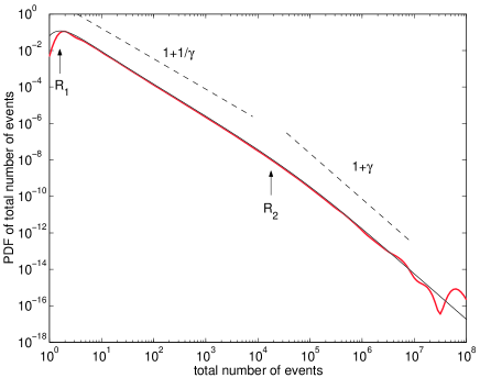
Figure 2: Numerical tests of the cross-over between (7) and (64) which is predicted by (59) of the PDF $p_{\mu}(r)$. The thick (resp. thin) line is the numerical simulation (resp. prediction (59)) for $n=0.97$ and $\gamma=1.5$. The two dashed lines outline the first intermediate asymptotic with exponent $1+1/\gamma$ for $R_{1}\ll r\ll R_{2}$ and truly asymptotic with exponent $1+\gamma$ for $r\gg R_{2}$. The crossovers $R_{1}=1.5$ and $R_{2}=1.6\times 10^{4}$ are defined by (60) and (63) respectively.

In the subcritical case ($n<1$), there is another power asymptotics. For $r\gg R_{1}$, one can rewrite (59) in the form

$$p_{\mu}(r)\simeq\frac{\mu}{[\gamma\Gamma(-\gamma)]^{1/\gamma}r^{\beta}}\,\varphi_{\gamma}\left(\frac{1-n}{\nu}r^{\frac{\gamma-1}{\gamma}}\right)\,.$$ (62)

If additionally $r\gg R_{2}$, where $R_{2}$ is defined by

$$R_{2}=\left(\frac{\nu}{1-n}\right)^{\gamma/(\gamma-1)}~{},$$ (63)

then, using the asymptotic (61) of $\varphi_{\gamma}(x)$, we obtain

$$p_{\mu}(r)\simeq\mu\,\gamma\,\left(\frac{n(\gamma-1)}{(1-n)\gamma}\right)^{\gamma+1}\,~{}~{}{1\over r^{1+\gamma}}\,,$$ (64)

for $r\gg\text{max}\{R_{1},R_{2}\}$. If additionally $R_{2}\gg R_{1}$, which holds if $\frac{1-n}{n}\ll(\gamma-1)\Gamma(-\gamma)\,\mu^{1-\gamma}$, then for $R_{1}\ll r\ll R_{2}$, there is an intermediate asymptotics following expression (7). These results are checked in Figure 2.

V Distribution of the total number of generations

We now turn to the determination of the PDF of the total number of branching generations, in other words, to the probability that the branching process terminates at a given generation number. Let $U_{\mu}(z;g)$ (respectively $U(z;g)$) denote the PGF corresponding to the number of daughters born from a mother with fertility $\mu$ (respectively with arbitrary fertility) at the $g$-th generation. A standard result of branching theory is Athreya

$$U_{\mu}(z;g+1)=G_{\mu}(U(z;g))~{};~{}U(z;g+1)=G(U(z;g)),$$ (65)

where $U(z;0)=z$. The probability that the branching process survives at the $g$-th generation is

$$p_{\mu}(g)=1-U_{\mu}(0,g)~{}.$$ (66)

The probability of termination of the branching process at the $g$-th generation is then given by

$$p_{g,\mu}(g)=p_{\mu}(g)-p_{\mu}(g+1)\,.$$ (67)

From (65,66), the probability for the branching process to survive at the $g$-th generation is

$$p_{\mu}(g+1)=1-G_{\mu}(1-p(g))\,.$$ (68)

$p(g)$ is the surviving probability at the $g$-th generation triggered by a mother of arbitrary fertility $\mu$, which obeys the recurrence

$$p(g+1)=1-G(1-p(g))\,,\qquad p(0)=1\,.$$ (69)

Equations (68) and (69) are easily solved numerically. We now extract the asymptotic power law behavior of $p_{g,\mu}(g)$. For small $p(g)$, the right-hand-side of (69) can be expanded as

$$1-G(1-p)\simeq np-\frac{C}{\gamma-1}p^{\gamma}-D~{}p^{2}\,,$$ (70)

where $C=n^{\gamma}\,\Gamma(2-\gamma)[(\gamma-1)/\gamma]^{\gamma}$ and $D=n^{2}\,(\gamma-1)^{2}/[2\gamma(\gamma-2)]$. For $\gamma>2$, it is enough to take the leading behavior of (70) up to second order in powers of $p$: $1-G(1-p)\simeq np-Dp^{2}$. With (69), this gives $p(g+1)-p(g)=-(1-n)p(g)-Dp^{2}$. Close to criticality $n\to 1$ for which a large number $g$ of generations occur, the leading behavior of the survival probability can be obtained by taking a continuous approximation to (69), giving $\frac{dp(g)}{dg}=-(1-n)p-D~{}p^{2}$. Its solution with initial condition $p(g_{0})=p_{0}$ has the form

$$p(g)=\frac{p_{0}(1-n)}{\displaystyle(1-n+p_{0}D)\,e^{(1-n)(g-g_{0})}-p_{0}D}\,.$$ (71)

Expression (71) gives a power law $p(g)\simeq 1/(D~{}g)$ for $1\ll g<1/(1-n)$ and crosses over to an exponential law for $g\geq 1/(1-n)$. Knowing $p(g)$, $p_{\mu}(g)$ given by (68) can be obtained. For instance, in the case of a Poisson distribution (16) giving (17), we obtain $p_{\mu}(g+1)=1-\exp\left[-\mu\,\kappa p(g)\right]$. For $\mu\kappa\,p(g)\ll 1$, $p_{\mu}(g+1)$ becomes $p_{\mu}(g+1)\simeq\mu\kappa\,p(g)$. The sought PDF of $p_{g,\mu}(g)$ defined by (67) is given by

$$p_{g,\mu}(g)\simeq\mu\kappa\,{dp(g)\over dg}\simeq{\mu\kappa\over D~{}g^{2}}.$$ (72)

The last equality holds for $g\geq 1/(1-n)$. This retrieves the standard mean field asymptotics $p_{g,\mu}(g)\sim 1/g^{2}$.

For $1<\gamma<2$, it is sufficient to keep only the following terms $1-G(1-p)\simeq np-\frac{C}{\gamma-1}p^{\gamma}$ in the expansion (70). Taking again a continuous approximation of (69) gives $\frac{dp(g)}{dg}=-(1-n)p-\frac{C}{\gamma-1}p^{\gamma}$, whose solution, for $g\ll 1/[(\gamma-1)(1-n)]$, reads

$$p(g)\simeq\left[p_{0}^{1-\gamma}+C(g-g_{0})\right]^{-1/(\gamma-1)}\sim{C\over(g-g_{0})}^{1/(\gamma-1)}~{},$$ (73)

Correspondingly, the PDF $p_{g,\mu}(g)$ that the number of generations is exactly $g$ is given by (7) with $C_{g}=\frac{\mu n}{\gamma}\,C^{-1/(\gamma-1)}$, valid for $\gamma$ not too close to $2$.

VI Concluding remarks

We have shown that the existence of cascades of triggered seismicity produces huge fluctuations of the total number of aftershocks and of the total number of generations from one sequence to another one for the same mainshock magnitude, characterized by power-law asymptotics. If the distribution of offsprings per mothers (of direct aftershocks per mainshock for seismicity) has a finite variance, we recover the well known mean-field results (9). In the case of an infinite variance relevant for earthquakes, we have discovered a new regime with exponents that varies continuously with the exponent $\gamma=b/\alpha$. The anomalous scaling reported here for $1<\gamma<2$ gives rise to less wild fluctuations in the total number of daughters from one mother to the next, compared with the mean field regime $\gamma\geq 2$. For instance, for earthquakes, we have probably $\gamma\approx 1.25$ for the preferred values $b\approx 1$ and $\alpha\approx 0.8$ alpha , which leads to $p_{r}(r)\sim 1/r^{1+0.8}$ and $p_{g}(g)\sim 1/g^{1+4}$ at $n=1$, compared with $p_{r}(r)\sim 1/r^{1+0.5}$ and $p_{g}(g)\sim 1/g^{1+1}$ for $\gamma\geq 2$. The reason for this behavior lies in the important role exerted by the mothers with the largest fertilities $\propto\mu$ on the rate of daughter births. In particular, this role explains why, away from criticality but close to it ($n\leq 1$), $p_{r}(r)$ crosses over from $1/r^{1+{1\over\gamma}}$ to $1/r^{1+\gamma}$ as $r$ increases: the latter asymptotic regime is nothing but the tail of the PDF (5) which controls the number of daughters born in the first generation from a mother with arbitrary fertility.

How relevant is the infinite variance regime $\gamma<2$ in view of the uncertainties in the exponents $\alpha$ and $b$? Indeed, the value of $\alpha$ is not only approximately known but its constancy (as a function of time) and uniformity (as a function of space) remains to be ascertained. In addition, the $b$-value also fluctuates and is typically in the range $0.75-1.25$ Frohlich . If we take the largest $b$-value of this interval ($b=1.25$), we remain in the infinite variance regime $\gamma<2$ as long as $\alpha>0.63$. Most present estimations discussed in section 2 give values above this lower bound. It thus seems that the results presented here should remain pertinent as more precise estimations of $\alpha$ and $b$ become available.

All these discussions assume untruncated power law distributions. However, it is well-known that the Gutenberg-Richter law exhibits an upper magnitude cut-off Kagan11 ; Pisor22 . By the logic leading to (4), this automatically implies also an upper fertility cut-off. This in turn removes the divergence of the variance for $\gamma<2$. How does this affect the distributions $p_{r}(r)$ and $p_{g}(g)$? This question is standard in the theory of power laws (see for instance Sorbook and references therein). Since the upper cutoff is very large so that the actual range of events is very large, our results obtained without truncation hold for a large range of values of $r$ and of $g$ respectively. However, the predicted power laws (7) have to cross-over to the mean-field ones (9) at threshold values beyond which the finiteness of the variance of fertilities become flagrant. In contrast, the presence of a lower cutoff magnitude benzion does not modify our results on the power law tail and has an influence only in shaping the bulk (small values) of the distributions.

The direct validation of our predictions (7) and (8) on earthquake catalogs is not feasible, due to the impossibility to distinguish aftershocks from uncorrelated events at large times after the mainshock, and due to the limited number of large aftershock sequences. Our results have however some consequences for the statistical properties of aftershock sequences. We have indeed shown in Bathlawpap that the existence of large fluctuations of the number of aftershocks per mainshock (summed over all generations) induces a non-trivial scaling of the difference in magnitude between a mainshock and its largest aftershock, so that Båth law can be recovered in the regime $b\gtrsim\alpha$. These results also suggest that the common use of a Poisson distribution in seismicity forecasts to model the distribution of the number of events within a finite space-time window is questionable, since the simple physics of cascades of earthquake triggering gives a very different (power law) distribution. Recent observations show non-Poisson power law distributions of seismic rates (see PG96 and work in progress). We suggest that these observations and our results could be used to improve earthquake forecasting by providing a more realistic distribution of the number of events.

Acknowledgments: We are grateful to two unknown referees and to Y. Ben-Zion as the editor, for useful remarks that helped improve the manuscript. This work is partially supported by NSF-EAR02-30429, by the Southern California Earthquake Center (SCEC) and by the James S. Mc Donnell Foundation 21st century scientist award/studying complex system. SCEC is funded by NSF Cooperative Agreement EAR-0106924 and USGS Cooperative Agreement 02HQAG0008. The SCEC contribution number for this paper is 741.

References

- (1) K.B. Athreya and P. Jagers, eds., Classical and modern branching processes (Springer, New York, 1997).
- (2) Ben-Zion, Y., Appendix 2, Key Formulas in Earthquake Seismology, in International Handbook of Earthquake and Engineering Seismology, Part B, 1857-1875, Academic Press, 2003.
- (3) G. Drakatos and J. Latoussakis, A catalog of aftershock sequences in Greece (1971-1997): Their spatial and temporal characteristics, J. Seismol. 5, 137-145 (2001).
- (4) Felzer, K.R., T.W. Becker, R.E. Abercrombie, G. Ekström and J.R. Rice, Triggering of the 1999 Hector Mine earthquake by aftershocks of the 1992 Landers earthquake, J. Geophys. Res., 107, doi:10.1029/2001JB000911, (2002).
- (5) K.R. Felzer, R.E. Abercrombie and G. Ekstrom, Secondary aftershocks and their importance for aftershock forecasting, Bull. Seis. Soc. Am., 93, 1433-1448 (2003).
- (6) C. Frohlich and S.D. Davis, Teleseismic values; or, much ado about 1.0, J. Geophys. Res., 98, 631-644 (1993).
- (7) K.I. Goh, Lee, D.S., Kahng, B. and Kim D., Sandpile on scale-free networks, 148701, Phys. Rev. Lett. 9114(14), 8701 (2003).
- (8) Guo and Y. Ogata, Statistical relations between the parameters of aftershocks in time, space, and magnitude, J. Geophys. Res. 102, 2857-2873 (1997).
- (9) A. Helmstetter, Is earthquake triggering driven by small earthquakes?, Phys. Rev. Lett. 91, 058501 (2003).
- (10) A. Helmstetter and D. Sornette, Sub-critical and supercritical regimes in epidemic models of earthquake aftershocks, J. Geophys. Res. 107, NO. B10, 2237, doi:10.1029/2001JB001580, (2002).
- (11) A. Helmstetter and D. Sornette, Bath’s law Derived from the Gutenberg-Richter law and from aftershock Properties, Geophys. Res. Lett., 30, 2069, 10.1029/2003GL018186 (2003)
- (12) A. Helmstetter and D. Sornette, Foreshocks explained by cascades of triggered seismicity, J. Geophys. Res. (Solid Earth) 108 (B10), 2457 10.1029/2003JB002409 01 (2003).
- (13) A. Helmstetter, D. Sornette and J.-R. Grasso, Mainshocks are aftershocks of conditional foreshocks: how do foreshock statistical properties emerge from aftershock laws, J. Geophys. Res., 108 (B10), 2046, doi:10.1029/2002JB001991 (2003).
- (14) Y.Y. Kagan, Likelihood analysis of earthquake catalogues, Geophys. J. Int. 106, 135-148 (1991).
- (15) Y.Y. Kagan, Universality of the seismic moment-frequency relation, Pure and Appl. Geophys. 155, 537-573 (1999).
- (16) Y.Y. Kagan and L. Knopoff, Stochastic synthesis of earthquake catalogs, J. Geophys. Res., 86, 2853 (1981).
- (17) Y.Y. Kagan and L. Knopoff, Statistical short-term earthquake prediction, Science, 236, 1563 (1987).
- (18) P. Major, The limit behaviour of elementary symmetric polynomials of i.i.d. random variables when their order tends to infinity, The Annals of Probability 27 (4), 1980-2010 (1999).
- (19) G.M. Molchan and O. E. Dmitrieva, Aftershock identification: methods and new approaches, Geophys. J. Int. 109, 501-516 (1992).
- (20) Y. Ogata, Statistical models for earthquake occurrence and residual analysis for point processes, J. Am. stat. Assoc. 83, 9 (1988).
- (21) Y. Ogata, Seismicity analysis through point-process modeling : a review, Pure Appl. Geophys.155, 471 (1999).
- (22) V. F. Pisarenko and T. Golubeva, The use of stable laws in seismicity models, Computational Seismology and Geodynamics 4, 127-137 (1996).
- (23) V.F. Pisarenko and D. Sornette, Characterization of the frequency of extreme events by the Generalized Pareto Distribution, Pure and Appl. Geophys. 160, 2343-2364 (2003).
- (24) G. Sankaranarayanan, Branching processes and its estimation theory (Wiley, New York, 1989).
- (25) S.K. Singh and G. Suarez, Regional variation in the number of aftershocks () of large, subduction-zone earthquakes (), Bull. Seism. Soc. Am. 78, 230-242 (1988).
- (26) A. Sornette and D. Sornette, Renormalization of earthquake aftershocks, Geophys. Res. Lett. 6, N13, 1981-1984 (1999).
- (27) D. Sornette, Critical Phenomena in Natural Sciences (Chaos, Fractals, Self-organization and Disorder: Concepts and Tools), second enlarged edition (Springer Series in Synergetics, Heidelberg, 2004)
- (28) D. Sornette and A. Helmstetter, Occurrence of finite-time-singularity in epidemic models of rupture, earthquakes and starquakes, Phys. Rev. Lett. 89, 158501 (2002).
- (29) D. Vere-Jones, A branching model for crack propagation, Pure Appl. Geophys. 114, 711-725 (1976).
- (30) D. Vere-Jones, Statistical theories of crack propagation, Math. Geol. 9, 455-481 (1977).
- (31) Y. Yamanaka and K. Shimazaki, Scaling relationship between the number of aftershocks and the size of the main shock, J. Phys. Earth 38, 305-324 (1990).
- (32) Zhuang, J., Ogata. Y. and Vere-Jones D., Analyzing earthquake clustering features by using stochastic reconstruction, in press in J. Geophys. Res., 2004.