ELECTRON-PHONON INTERACTION IN ULTRASMALL-RADIUS CARBON NANOTUBES

Abstract

We perform analysis of the band structure, phonon dispersion, and electron-phonon interactions in three types of small-radius carbon nanotubes. We find that the (5,5) can be described well by the zone-folding method and the electron-phonon interaction is too small to support either a charge-density wave or superconductivity at realistic temperatures. For ultra-small (5,0) and (6,0) nanotubes we find that the large curvature makes these tubes metallic with a large density of states at the Fermi energy and leads to unusual electron-phonon interactions, with the dominant coupling coming from the out-of-plane phonon modes. By combining the frozen-phonon approximation with the RPA analysis of the giant Kohn anomaly in 1d we find parameters of the effective Frölich Hamiltonian for the conduction electrons. Neglecting Coulomb interactions, we find that the (5,5) CNT remains stable to instabilities of the Fermi surface down to very low temperatures while for the (5,0) and (6,0) CNTs a CDW instability will occur. When we include a realistic model of Coulomb interaction we find that the charge-density wave remains dominant in the (6,0) CNT with $T_{\rm CDW}$ around 5 K while the charge-density wave instability is suppressed to very low temperatures in the (5,0) CNT, making superconductivity dominant with transition temperature around one Kelvin.

I INTRODUCTION

It has been over a decade since the discovery of carbon nanotubes (CNTs) Ijima91 and the interest level in these systems continues to be high. The majority of theoretical work on CNTs focuses on understanding the effects of the electron-electron interactions using the celebrated Luttinger liquid theory.Egger00 Experimental observation of superconductivity in ropes of nanotubes Kociak01 and small-radius nanotubes in a zeolite matrix Tang01 has also motivated theoretical studies of the electron-phonon interactions (EPI), including the analysis of charge density wave (CDW) Mintmire92 ; Huang96 ; Sedeki00 ; Dubay02 and superconducting (SC) Benedict95 ; Sedeki02 ; Byczuk02 ; Gonzalez02 ; Kamide03 instabilities. In this work we study the electron-phonon interactions in CNTs and discuss possible instabilities to the CDW and SC orders. Our approach provides reliable parameters for the effective Hamiltonians we use in contrast to the Luttinger liquid treatments where obtaining such accurate quantities is quite difficult.

A conventional starting point for discussing the electron-phonon interaction in solids is the Frölich Hamiltonian Schrieffer64

$${\cal H} = \sum_{k\tau\sigma}\varepsilon_{k\tau}c_{k\tau\sigma}^{\dagger}c_{k\tau\sigma}+\sum_{q\mu}\Omega^{0}_{q\mu}(a_{q\mu}^{\dagger}a_{q\mu}+\frac{1}{2})$$ (1)

$$+ \sum_{k\tau k^{\prime}\tau^{\prime}\sigma\mu}g_{k\tau k^{\prime}\tau^{\prime}\mu}c_{k\tau\sigma}^{\dagger}c_{k^{\prime}\tau^{\prime}\sigma}(a_{q\mu}+a_{-q\mu}^{\dagger}).$$

Here $c^{\dagger}_{k\tau\sigma}$ creates an electron with quasimomentum $k$ in band $\tau$ with spin $\sigma$, $a^{\dagger}_{q\mu}$ creates a phonon with lattice momentum $q$ and polarization $\mu$, and $q=k-k^{\prime}$ modulo a reciprocal lattice vector. The energies of electron quasiparticles and phonons (in the absence of EPC) are given by $\varepsilon_{k\tau}$ and $\Omega^{0}_{q\mu}$ respectively. The EPC vertex is given by

$$g_{k\tau k^{\prime}\tau^{\prime}\mu}=\sqrt{\frac{1}{2\Omega^{0}_{q}MNN_{c}}}M_{k\tau k^{\prime}\tau^{\prime}\mu}$$ (2)

with

$$M_{k\tau k^{\prime}\tau^{\prime}\mu}=N\langle{\psi_{k\tau}}|\sum_{i}\frac{\partial V}{\partial{\bf R}_{0i}}\cdot\hat{\epsilon}_{q\mu}(i)|{\psi_{k^{\prime}\tau^{\prime}}}\rangle.$$ (3)

Here $|{\psi_{k\tau}}\rangle=c^{\dagger}_{k\tau}|{0}\rangle$ is a quasistationary electron state in band $\tau$ with quasimomentum $k$, $\hat{\epsilon}_{q\mu}(i)$ is the phonon polarization vector on atom $i$ in the unit cell, $N_{c}$ is the number of atoms per unit cell, $M$ is the mass of a single C atom, $N$ is the total number of unit cells in the system, and $\frac{\delta V}{\delta{\bf R}_{0i}}$ is the derivative of the crystal potential with respect to the ion position ${\bf R}_{0i}$.

A common approach to obtaining parameters of the Hamiltonian Eq. (1) for the CNTs is the zone-folding method (ZFM). Saito98 The essence of this method is to take the electron band structure and the phonon dispersion for graphene and quantize momenta in the direction of the wrapping. The main results of such a procedure may be summarized as follows. The only bands crossing the Fermi level in graphene are the bonding and the antibonding combinations of the atomic $p_{z}$ orbitals. Hence, the zone-folding method predicts that these are the only bands which may cross the Fermi level in carbon nanotubes. The condition for the quantized momenta to cross the Dirac points of the graphene gives the condition for the (N,M) CNT to be metallic: $N-M$ should be divisible by 3. The ZFM also predicts that the electron-phonon coupling in the CNTs should be dominated by the in-plane optical modes. This follows from the fact that the latter have the largest effect on the overlaps between the $p_{z}$ orbitals of the neighboring carbon atoms.

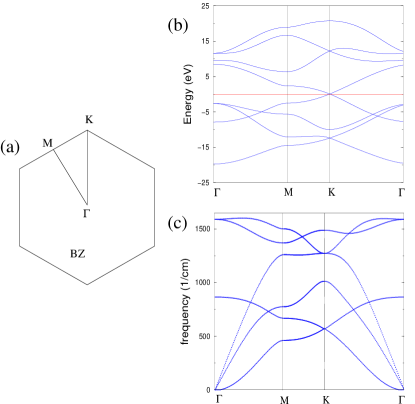
Figure 1: The first Brillouin zone (a), electronic band structure (b), and phonon dispersion (c) of graphene.

While the ZFM was shown to provide a quantitatively accurate description of the larger radius nanotubes, it is expected to fail as the radius of the nanotubes is decreased and the curvature of the C-C bonds becomes important. Determining the band structure, the phonon dispersion, and the electron-phonon coupling of the small radius CNTs requires detailed microscopic calculations. In this paper we use the empirical tight-binding model Mehl96 to provide such analysis for three types of small-radius nanotubes: (5,0) with the diameter 3.9 Å, (6,0) with the diameter 4.7 Å, and (5,5) with the diameter 6.8 Å. We find that the large curvature of the C-C bonds leads to qualitative changes in the band structure of the (5,0) and (6,0) nanotubes (band structures of the (6,0) and (7,0) nanotubes have been discussed previously in Blase94 ). For example, the (5,0) CNT becomes metallic from strong hybridization between the $\sigma$ and $\pi$ bands (see Fig. 4). Frequencies of the phonon modes in small radius CNTs are also strongly renormalized from their values in graphene. Not only does the out-of-plane acoustic mode become a finite frequency breathing mode, Saito98 but even the optical modes change their energy appreciably (see e.g. Fig. 7). Finally, the electron-phonon coupling changes qualitatively in the small-radius CNTs. It is no longer dominated by the in-plane optical modes but by the out-of-plane optical modes which oscillate between the $sp_{2}$ bonding of graphene and the $sp_{3}$ bonding of diamond (see discussion in Sec. VI). We find that the strong effects of the CNT curvature decrease rapidly with increasing the tube radius. Already for the (5,5) nanotubes the ZFM gives a fairly accurate description of the band structure as well as the electron-phonon interactions.

Determining parameters of the Frölich Hamiltonian for a one-dimensional system is not as straightfoward as for two and three-dimensional metals. Traditional methods for analyzing EPI from first-principles calculations are mean-field and, therefore, suffer from instabilities intrinsic to one-dimensional systems. In particular, the frozen-phonon approximation, which is commonly used to determine the phonon frequencies, $\Omega^{0}_{q\mu}$, in Eq. (1) gives imaginary frequencies close to the nesting wave vector $q=2k_{F}$. This is the result of the giant Kohn anomaly, Kohn59 which corresponds to the Peierls instability of the one-dimensional electron-phonon system.Peierls55 An important result of our paper is that we developed a new formalism, which combines the frozen-phonon approximation with the Random-Phase Approximation (RPA) analysis of the EPI. This allows us to extract effective non-singular parameters of the Frölich Hamiltonian from first-principles calculations or from the empirical tight-binding model. This technique should be applicable to many systems other than carbon nanotubes.

After determining parameters of the Frölich Hamiltonian Eq. (1) for the (5,0), (6,0), and (5,5) CNTs we discuss possible superconducting and charge-density wave instabilities in these systems. We find that neglecting the residual Coulomb interaction leads to much stronger CDW instabilities in all three cases (in such analysis Coulomb interaction is included only at the mean-field level via the energy of the single-particle quasi-stationary states, $\varepsilon_{k\tau}$). In the mean-field approximation we find the onset of the Peierls instability at temperatures 160, 5, and $10^{-14}$ K for (5,0), (6,0), and (5,5) CNTs respectively. However, including the Coulomb interactions at the RPA level Levin74 can lead to a stronger suppression of the CDW transition temperatures, $T_{\rm CDW}$, than the superconducting $T_{\rm SC}$. For instance, we find by using the model Coulomb interaction of Ref. Egger98, that for the (5,0) CNT, the CDW transition is suppressed to very low temperatures while superconductivity becomes the dominant phase with transition temperature of $T_{\rm SC}\approx 1$ K.

This paper is organized as follows. In Sec. II we discuss our method for extracting parameters for the one-dimensional Frölich Hamiltonian. We then apply this method to the (5,0), (6,0), and (5,5) CNTs in Sec. III. In Sec. IV, we use the constructed Hamiltonian for these CNTs to study their instabilities toward superconductivity and charge-density wave states. The effect of introducing the residual Coulomb interacting between electrons is covered in Sec. V. Finally all of the results are discussed and summarized in Sec. VI.

II EXTRACTING PARAMETERS OF THE EFFECTIVE FRÖLICH HAMILTONIAN FROM THE FIRST PRINCIPLE CALCULATIONS

Now we discuss our methods for calculating input parameters to the Frölich Hamiltonian Eq. (1) for the representative nanotubes. Our analysis relies on the the empirical tight-binding model Mehl96 but it is easily amenable to any density-functional theory Hohenberg64 ; Kohn65 treatment of the system.

II.1 Band Structure

To compute the electronic structure of the CNTs we study, we use the NRL tight-binding method Mehl96 which has been tested and provided accurate results on a variety of materials. In this method, the Slater-Koster tight-binding matrix elements are parametrized and are fit to reproduce the first-principles density-functional band structures and total energies, with around 70 adjustable parameters per element.

We study the (5,0), (6,0), and (5,5) CNTs which are shown in Figs. 4,8, and 10. The smallest possible unit cells for these CNTs contain 20, 24, and 20 atoms respectively. These CNTs are relaxed by minimizing their total energy per unit cell with respect to the atomic coordinates using 35 k-points in the first Brillouin zone. Matrix elements between neighboring atoms of up to 5.5 Å were used. The calculations were performed on an orthorhombic lattice with spacing between parallel CNTs of 16 Å, a distance sufficiently large to ensure negligible dispersion from inter-tube hopping. Once the CNTs are relaxed, the band structure is calculated.

II.2 The phonon modes

To calculate the electron-phonon coupling vertices and the phonon frequencies which will be discussed in the subsequent sections, one needs to have the ionic displacements corresponding to the normal vibrational modes of the CNT. As pointed out previously, Sanchez-Portal99; Saito98 we find that it is typically sufficient to use the zone-folded modes of a graphene sheet, even for the small-radius CNTs we study as will be discussed below.

Following the method used in the book of Saito et al., Saito98 we have computed the $60\times 60$ dynamical matrix of a (5,0) CNT and in Fig. 2 we compare the resulting phonon dispersions with the zone-folding results. The ionic displacement modes obtained by the two different methods are very similar except for a few special cases. For instance, the zone-folding results give three acoustic modes which correspond to translating the graphene sheet in different directions. Upon rolling the graphene sheet, these modes get mapped to two acoustic modes corresponding to rotation about the CNT axis and translation along the CNT axis and the optical breathing mode. Conversely, diagonalizing the dynamical matrix of the CNT gives four acoustic modes corresponding to translations in three directions and the rotating mode (actually using the method of Ref. Saito98, , one obtains a small spurious frequency for the rotating mode as pointed in this reference). Upon unrolling the CNT to the graphene sheet, the rotating mode and the mode corresponding to translation along the CNT axis will become acoustic modes of the graphene sheet. However, the two CNT translational modes which are perpendicular to the CNT axis will get mapped to ionic displacements which are not eigenmodes of the graphene sheet which are mixtures of in-plane and out-of-plane oscillations. In addition, using the dynamical matrix of the CNT, we find that there is mixing between the breathing and strething modes around $k=0.3$. In this vicinity, there is level repulsion from the lifting of the degeneracy of these modes. Away from this point, the modes are, to a good approximation, decoupled.

In our analysis of the electron-phonon coupling we use the displacements obtained from the zone-folding method to simplify the calculations, as well as to give a clear conceptual picture. We then check that none of the important electron-phonon couplings come from any of the few graphene modes for which the zone-folding method breaks down.

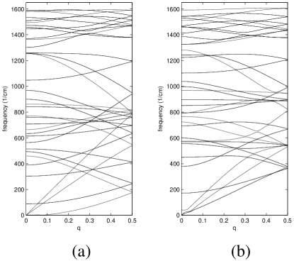
Figure 2: The phonon dispersions of a (5,0) CNT determined by (a) the zone-folding method and (b) diagonalizing the full dynamical matrix of the CNT.

II.3 The electron-phonon coupling vertices

The electron-phonon coupling (EPC) matrix in Eq. (3) can be evaluated by using the finite difference formula

$$M_{k\tau k^{\prime}\tau^{\prime}\mu}=\frac{1}{u}\langle{\psi_{k\tau}}|(V_{q\mu}-V_{0})|{\psi_{k^{\prime}\tau^{\prime}}}\rangle$$ (4)

where $V_{q\mu}$ and $V_{0}$ are the perturbed and the unperturbed lattice potentials respectively. A method for calculating the expression (4) with a plane-wave basis set was previously developed.Lam86 In this paper we extend this procedure to tight-binding models. We introduce the standard tight-binding notation

$$|{\psi_{k\tau}}\rangle=\sum_{il}A_{k\tau il}|{\chi_{kil}}\rangle.$$ (5)

$$|{\chi_{kil}}\rangle=\frac{1}{\sqrt{N}}\sum_{n}e^{ik\cdot R_{n}}|{\phi_{nil}}\rangle.$$ (6)

Here $|{\phi_{ni}}\rangle$ are the electron states for isolated carbon atoms, $n$ runs over unit cells, $i$ runs over basis vectors in the unit cell, and $l$ runs over orbital type. We find (for details, see Appendix A)

$$M_{k\tau k^{\prime}\tau^{\prime}\mu}=\frac{1}{u}\sum_{ili^{\prime}l^{\prime}}A^{*}_{k\tau il}\langle{\chi_{kil}^{q\mu}}|({\cal H}^{q\mu}-E_{F})|{\chi_{k^{\prime}i^{\prime}l^{\prime}}^{q\mu}}\rangle A_{k^{\prime}\tau^{\prime}i^{\prime}l^{\prime}}.$$ (7)

This expression can be computed by evaluating the tight-binding Hamiltonian and overlap matrices for the distorted lattice, evaluating the coefficients $A_{ki}$ and $A_{k^{\prime}i^{\prime}}$ of the wave functions for the undistorted lattice, and performing the above sum.

In all the calculations presented in this paper we used the ZFM to find phonon eigenvectors in the nanotubes starting from the phonon eigenvectors in graphene.Saito98 The latter have been obtained using the $6\times 6$ dynamical matrix of graphene given in Ref. Jishi93, . We emphasize that we use the ZFM only to find the phonon eigenvectors in small nanotubes, but not the phonon frequencies. The frequencies are affected strongly by the CNT curvature, and should be computed directly. This is discussed in detail in Sec. II.4 and Sec. III.

II.4 Phonon frequencies

A standard method of calculating the bare phonon frequencies $\Omega_{q\mu}^{0}$ in Eq. (1) is the frozen-phonon approximation (FPA).Yin82 In this approach

$$\Omega_{q\mu}=\frac{1}{u\sqrt{MN_{c}}}\sqrt{\Delta E_{\cos}(q)+\Delta E_{\sin}(q)}$$ (8)

where $u$ is the amplitude of the displacement, and $\Delta E_{\cos}(q)$ and $\Delta E_{\sin}(q)$ are the energy differences per unit cell between the distorted and equilibrium lattice structures where the distortion corresponds to the real and imaginary parts of $\delta{\bf R}_{ni}=ue^{iqR_{n}}\hat{\epsilon}_{q\mu}(i)$ respectively. When we apply this procedure to one-dimensional CNTs, we find that $\Delta E_{\cos}(q)+\Delta E_{\sin}(q)$ becomes negative around certain wave vectors (see e.g. Fig. 7). A closer inspection shows that such anomalous softening always corresponds to one of the $2k_{F}$ wave vectors of the electron bands indicating the presence of the giant Kohn anomaly.

It is important to realize that the divergence of $\Omega_{q\mu}$ obtained in the FPA does not imply the divergence of $\Omega^{0}_{q\mu}$ in the Frölich Hamiltonian Eq. (1). The frequencies $\Omega_{q\mu}$ are calculated after the electron-phonon interaction in Eq. (1) have been included, which gives anomalous softening at $2k_{F}$ due to the well-known Peierls instability of electron-phonon systems in 1d. In two and three dimensional systems renormalization of the phonon frequency by electrons in the conduction band is typically negligible. So, one can use phonon energies obtained in the FPA as a direct input into the Frölich Hamiltonian. By contrast, nesting of the one-dimensional Fermi surfaces, leads to dramatic renormalization of the phonon dispersion by electrons in the conduction band.

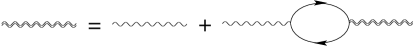
Figure 3: The phonon propagator evaluated within the RPA.

To extract the bare phonon frequency $\Omega^{0}_{q\mu}$ from the numerically computed $\Omega_{q\mu}$, we point out a connection between the FPA and the RPA for the Frölich Hamiltonian. For negligible interband coupling (this condition is satisfied for all modes showing the giant Kohn anomaly, which we discuss in this paper) Dyson’s equation for the phonon propagator $D(q,i\nu_{m})$, as shown in 3 is given by

$$D_{\mu}(q,i\nu_{m})=D_{0\mu}(q,i\nu_{m})\left(1+\Pi_{\mu}(q,i\nu_{m})D_{\mu}(q,i\nu_{m})\right).$$ (9)

Here $\nu_{m}=2\pi mT$ are the bosonic Matsubara frequencies and

$$D_{0\mu}(q,i\nu_{m})=\frac{2\Omega_{q\mu}}{(i\nu_{m})^{2}-(\Omega_{q\mu}^{0})^{2}}.$$ (10)

is the non-interacting phonon Green’s function. The phonon self-energy evaluated in the RPA is given by

$$\Pi_{\mu}(q,i\nu_{m})=2T\sum_{np\tau}|g_{p\tau p+q\tau\mu}|^{2}G_{0\tau}(p+q,i\omega_{m+n})G_{0\tau}(p,i\omega_{n}).$$ (11)

where non-interacting electronic Green’s functions are given by $G_{0\tau}(p,i\omega_{n})=(i\omega_{n}-\varepsilon_{p\tau})^{-1}$ and $\omega_{n}=\pi(2n+1)T$ for integer $n$ are the fermionic Matsubara frequencies. Summing over $n$, we obtain for Eq. (11)

$$\Pi_{\mu}(q,i\nu_{m})=2\sum_{\tau}|g_{q\tau\mu}|^{2}\chi_{0\tau}(q,i\nu_{m})$$ (12)

where the bare susceptibility is given by

$$\chi_{0\tau}(q,i\nu_{m})=\sum_{p}\frac{f(\varepsilon_{p\tau})-f(\varepsilon_{p+q\tau})}{i\nu_{m}+\varepsilon_{p\tau}-\varepsilon_{p+q\tau}}.$$ (13)

with $f(\varepsilon_{p\tau})=(1+e^{\beta\varepsilon_{p\tau}})^{-1}$ being the Fermi-Dirac distribution function.

The poles of the phonon Green’s function $\Omega_{q\mu}$ (we put $i\nu_{m}\rightarrow\Omega_{q\mu}$ in $D_{\mu}(q,i\nu_{m})$), which give the dressed phonon frequencies, will satisfy the equation

$$\left(\Omega_{q\mu}\right)_{\rm RPA}^{2}=\left(\Omega_{q\mu}^{0}\right)^{2}+2\Omega^{0}_{q\mu}\Pi_{\mu}(q,\Omega_{q\mu}).$$ (14)

Due to the large energy difference between electrons and phonons, it is typically a good approximation to set $\Omega_{q\mu}\rightarrow 0$ in $\Pi_{\mu}(q,\Omega_{q\mu})$. This approximation results in an expression that can be derived by doing stationary second-order perturbation theory to obtain the change in energy due to the presence of the phonon. That is, setting $\Omega_{q\mu}\rightarrow 0$ in $\Pi(q,\Omega_{q\mu})$ corresponds to the frozen-phonon approximation

$$\left(\Omega_{q\mu}\right)_{\rm FPA}^{2}=\left(\Omega_{q\mu}^{0}\right)^{2}+2\Omega^{0}_{q\mu}\Pi_{\mu}(q,0).$$ (15)

We can typically approximate well the quasiparticle energy by a plane-wave state with given effective mass $m^{*}$. Then, by incorporating the FPA, at zero temperature the integral in Eq. (13) can be done which will enable us to obtain

$$\left(\Omega_{q\mu}\right)_{\rm FPA}^{2}=\left(\Omega_{q\mu}^{0}\right)^{2}$$ (16)

$$+ \sum_{\tau}|M_{2k_{\rm F}\tau\mu}|^{2}\frac{2m^{*}a}{\pi MN_{c}k_{{\rm F}\tau}}\log\left|\frac{2k_{{\rm F}\tau}-q}{2k_{{\rm F}\tau}+q}\right|$$

This expression explicitly shows the logarithmic divergences in the phonon dispersion at the nesting wave vectors of the Fermi surface. This is the famous Peierls instability to a CDW state. Our procedure for determining the elusive undressed frequencies is then as follows. We take $\Omega_{q\mu}$ obtained from the FPA and fit them with the expression Eq. (16) using $\Omega_{q\mu}^{0}$ as an adjustable parameter. The coefficients of the log divergences at the nesting wave vectors of the Fermi surface are fixed by the effective masses $m_{\tau}^{*}$ and $k_{{\rm F}\tau}$ (known from the band structure) and the computed EPC matrix elements $M_{2k_{F}\tau\mu}$. In all cases we found excellent agreement of the calculated FPA frequencies with Eq. (16) in the vicinity of the singular points, which provides a good self-consistency check for our analysis.

III RESULTS FOR REPRESENTATIVE NANOTUBES

III.1 (5,0) nanotube

The zig-zag (5,0) CNT has a diameter of around 3.9 Å making it close to the theoretical limit.Peng00 Nanotubes of this size have been experimentally realized through growth in the channels of a zeolite host.Tang01 Through the Raman measurement of the frequency of the radial breathing mode, the (5,0) CNT is thought to be a likely candidate structure for these experiments.Li01

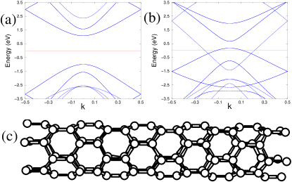
Figure 4: The band structure of the (5,0) CNT obtained through zone-folding (a) and calculated directly (b) along with the atomic structure (c).

We first compute the band structure of this tube by using the zone-folding method.Saito98 To do this, we use the band structure of graphene, which is shown in Fig. 1, computed by using the NRL tight binding method. Shown in this figure are four valence bands and four conduction bands, coming from the three $sp_{2}$ and one $p_{z}$ bonding and antibonding states respectively. There is a degeneracy between the $p_{z}$ bonding and antibonding states at the Fermi energy at the $K$ point in the first Brillouin zone which accounts for the semimetallic behavior of graphene. The zone-folding band structure of the (5,0) CNT is shown in the right of Fig. 4. Since $5/3$ is not an, zone-folding predicts this CNT to be semiconducting.

Fig. 4 (b) shows the band structure of the (5,0) CNT calculated directly by using a unit cell of 20 atoms. One sees that there are significant qualitative differences between the two band structures, one being that the directly computed band structure predicts metallic behavior. The inner band (with smaller Fermi point $k_{F}^{\rm A}$) is doubly degenerate while the outer band (with larger Fermi point $k_{F}^{\rm B}$) is nondegenerate. The strong curvature effects causes hybridization between $\sigma$ and $\pi$ bands, pushing them through the Fermi energy and therefore making the tube metallic. Furthermore, for the (5,0) CNT, we see that inner band is close to the Van Hove singularity at $k=0$, which produces a large density of states at the Fermi energy. The calculated density of $\nu(0)=0.16$ states/ eV / C atom is around a factor of five larger than that of larger radius metallic armchair CNTs.

After the band structure is calculated, we consider all possible scattering processes of electrons between Fermi points $-k_{F}^{\rm B},-k_{F}^{\rm A},k_{F}^{\rm A}$, and $k_{F}^{\rm B}$ due to phonons with wave vectors $q$ that satisfy the momentum conservation condition. As a starting point for the phonon spectrum, we use the dynamical matrix of Jishi et al. Jishi93 which uses a fourth nearest-neighbor model, and we employ the zone-folding method. The reproduced phonon dispersion of graphene is shown in Fig. 1. For a given process, we calculate the coupling for all of the $3\times N_{c}$ distinct phonon modes where $N_{c}=20$ is the number of atoms per unit cell. Shown in Fig. 5 is an example of the outcome for one of these calculations. Shown is the coupling for the outer band $2k_{F}^{\rm A}$ processes vs. graphene frequency. One can immediately see that most couplings vanish which can be explained by symmetry of the electronic wave functions and the phonon modes.

Figure 5: The coupling $M_{kk^{\prime}}$ for the outer band $2k_{F}^{\rm B}$ process for each of the 3 $\times$ 20 = 60 phonon modes respectively vs. graphene frequency.

To keep this paper concise, we cannot present all of the coupling results for each scattering process. Instead, we show the most dominant couplings. These dominant couplings were found to be from intraband $2k_{F}$ processes. The largest couplings for the (5,0) CNT occur for phonons along the $\Gamma M$ line of graphene at the appropriate wave vector corresponding to the particular $2k_{F}$. For the inner band, the largest couplings, in descending order, occur for the out-of-plane optical mode, the radial breathing mode, and the in-plane acoustic stretching mode. For the outer (with larger $k_{F}$) band, the dominant couplings occur for the out-of-plane optical, an in-plane optical, the radial breathing, and in-plane stretching modes. These results are summarized in Fig. 6 and Table 1. Although the magnitunde of the dominant coupling matrix element for the outer band is larger than that of the inner band, the inner band processes are significantly more important in the study of instabilities because their contribution to the total density of states at the Fermi energy is significantly larger than that of the outer band. This is due to the small Fermi velocity of the inner band and its degeneracy.

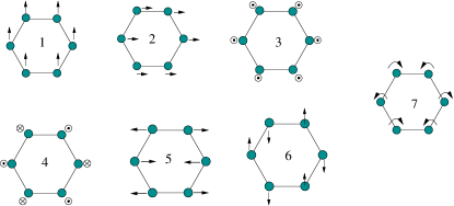
Figure 6: 1-6: The phonon modes at the $\Gamma$ point in the first Brillouin zone of graphene. 7: An in-plane optical phonon mode at the $K$ point of the first Brillouin zone of graphene. The out-of-plane optical mode 4 is the leading cause of the CDW instability in the (5,0) and (6,0) CNTs.

(5,0)	mode	$\omega_{q}^{graph}$ (cm-1)	$M_{kk^{\prime}}$(eV/Å)
$2k_{F}^{\rm A}$	4	853	5.55
	3	39	4.46
	5	1588	4.24
$2k_{F}^{\rm B}$	4	829	8.56
	5	1593	5.23
	3	133	4.97
	2	684	4.10

Table 1: Calculated values for the dominant coupling processes for the (5,0) CNT. The numbering scheme here corresponds to that given in Fig. 6. $2k_{F}^{\rm A}$ and $2k_{F}^{\rm B}$ correspond to inner and outer band processes respectively. Phonon frequencies are given for graphene.

It is interesting to note that the phonons that have the strongest coupling to electrons at the Fermi surface are out-of-plane modes. This is different than intercalated graphene where in-plane phonon modes are responsible for superconductivity.Dresselhaus81 The fact that the out-of-plane modes are the most important for this CNT are presumably due to the large curvature effects. For instance, we find that the bond angles of the relaxed (5,0) CNT structure (having the values of $119.4^{\circ}$ and $111.9^{\circ}$)are intermediate between the $sp_{2}$ bond angle (found in graphene) of $120^{\circ}$ and the $sp_{3}$ bond angles (found in diamond) of $109.4^{\circ}$.

Now we calculate the CNT phonon frequencies by using the frozen-phonon approximation with the eigenvectors from graphene. The circles shown in Fig. 7 are the frequencies obtained for phonon modes along the $\Gamma M$ line of graphene for the out-of-plane optical mode which was found to be the most important mode. First, we see that the calculated FPA frequencies are significantly lower than the corresponding ones in graphene. This can be understood as follows. The strong curvature of the nanotube changes the C-C bonds so that they are in an intermediate regime between the $sp_{2}$ bonding (found in graphene) and $sp_{3}$ bonding (found in diamond). The out-of-plane optical mode oscillates between these two bonding configurations and is therefore significantly softened. Next, we notice that there are divergences at $q=2k_{F}^{\rm A}$ and $q=2k_{F}^{\rm B}$. This result is the giant Kohn anomaly.

Figure 7: (a): Phonon dispersion for the (5,0) CNT along the $\Gamma M$ line of graphene. The X’s denote values for which the frozen-phonon approximation gave imaginary frequencies for the out-of-plane optical mode in the vicinity of $2k_{F}^{\rm A}$. (b): The mode showing the most softening fit to the RPA expression.

To extract the bare phonon frequency of the Frölich Hamiltonian Eq. 1 for the (5,0) CNT we follow the procedure discussed in Sec. II.4. The dressed phonon frequencies are given by

$$\left(\Omega_{q\mu}\right)^{2}=\left(\Omega_{q\mu}^{0}\right)^{2} + D_{\rm A}\log\left|\frac{2k_{F}^{\rm A}-q}{2k_{F}^{\rm A}+q}\right|$$

$$+ D_{\rm B}\log\left|\frac{2k_{F}^{\rm B}-q}{2k_{F}^{\rm B}+q}\right|.$$

where

$$D_{\rm A}=|M_{2k_{F}^{\rm A}}|^{2}\frac{2m_{\rm A}^{*}a}{\pi MN_{c}k_{F}^{\rm A}}$$ (18)

and

$$D_{\rm B}=|M_{2k_{F}^{\rm B}}|^{2}\frac{m_{\rm B}^{*}a}{\pi MN_{c}k_{F}^{\rm B}}$$ (19)

All of the quantities needed to calculate the coefficients $D_{\rm A}$ and $D_{\rm B}$have been obtained already. We assume that the bare phonon frequencies are fit well by the form $(\Omega_{q\mu}^{0})^{2}=a_{0}+a_{1}q+a_{2}q^{2}$. We then use $a_{0},a_{1}$ and $a_{2}$ as fitting parameters to fit our expression for $\Omega_{q}$ to the calculated FPA frequencies. Doing this thereby enables us to extract the important bare frequency dispersion $\Omega_{q}^{0}$ which is shown in Fig. 7. Extracting these bare frequencies $\Omega_{q}^{0}$ allows us to calibrate the effective Frölich Hamiltonian Eq. (1) which will be used to study instabilities of the electron-phonon system. With our previously calculated quantities, we obtain $D_{\rm A}=(219$ cm${}^{-1})^{2}$ and $D_{\rm B}=(146$ cm${}^{-1})^{2}$. Using these values we thereby extract $\Omega_{q=2k_{F}^{\rm A}}^{0}=433$ cm^-1.

III.2 (6,0) nanotube

The band structure of the (6,0) CNT was considered extensively by Blase et al. in Ref. Blase94, . This tube has a slightly larger diameter of 4.7 Å. The zone-folding band structure of this CNT is shown in the left of Fig. 8. As is typical of metallic zig-zag tubes, there are two bands crossing at $k=0$ at the Fermi energy. The band structure directly computed with 24 atoms in the unit cell is shown in the right of Fig. 8. As discussed before Blase94 , these band structures differ qualitatively which is a result of the hybridization of the $sp_{2}$ and $p_{z}$ bands. Here the inner band (with smaller $k_{F}^{\rm B}$) is nondegenerate and originates from the $p_{z}$ bonds in graphene while the outer band (with larger $k_{F}^{\rm A}$) is degenerate and originates from the $sp_{2}$ bonds in graphene.

The coupling matrix elements for the (6,0) CNT were computed and the coupling for the most dominant modes are shown in Fig. 6 and Table 2. The dominant inner band couplings were for intraband processes and are, in descending order, to the out-of-plane optical and an in-plane optical. The dominant outer band couplings processes were found to be the out-of-plane optical mode, an in-plane optical mode, the radial breathing mode, and the in-plane acoustic stretching mode.

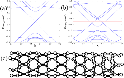
Figure 8: The band structure of the (6,0) CNT obtained through zone-folding (a) and calculated directly (b) along with the atomic structure (c).

(6,0)	mode	$\omega^{graph}_{q}$ (cm-1)	$M_{kk^{\prime}}$(eV/Å)
$2k_{F}^{\rm A}$	4	857	7.27
	5	1585	6.80
$2k_{F}^{\rm B}$	4	847	6.84
	6	1591	6.12
	3	68	3.73
	2	493	2.31

Table 2: Calculated values for the dominant coupling processes for the (6,0) CNT. The numbering scheme here corresponds to that given in Fig. 6. $2k_{F}^{\rm A}$ and $2k_{F}^{\rm B}$ correspond to inner and outer band processes respectively. Phonon frequencies are given for graphene.

Figure 9: (a): Phonon dispersion for the (6,0) CNT along the $\Gamma M$ line of graphene. (b): The mode showing the most softening fit to the RPA expression.

Using the same procedure as was used for the (5,0) CNT in the previous section for extracting the bare phonon frequency at $2k_{F}^{\rm A}$. From the previously computed values for the electron-phonon coupling matrix elements and the band structure, we find $D_{\rm A}=(166$ cm${}^{-1})^{2}$ and $D_{\rm B}=(107$ cm${}^{-1})^{2}$. After fitting, we extract the value $\Omega_{q=2k_{F}^{\rm A}}^{0}=480$ cm^-1.

III.3 (5,5) nanotube

Finally, we study the more conventional armchair (5,5) CNT which has a diameter of around 6.8 Å. As shown in Fig. 10, the zone-folding and directly computed band structure for this larger diameter tube agree quite will. Both of these band structures show two bands which originate from $p_{z}$ orbitals which cross at the Fermi energy at around $k=\frac{2}{3}\frac{a}{\pi}$.

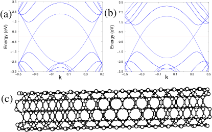
Figure 10: The band structure of the (5,5) CNT obtained through zone-folding and calculated directly are shown in the upper right and left. Bottom: the structure of the (5,5) CNT.

The largest couplings for the CNT were found to again be from the intraband processes and are shown in Fig. 6 and Table 3. The only significant intraband coupling is for an in-plane mode shown denoted by 7 in Fig. 6. The wave vector for this mode is at the $K$ point in the first Brillouin zone of graphene. For the interband processes, there is coupling to the the radial breathing mode, but this is significantly smaller.

(5,5)	mode	$\omega^{graph}_{q}$ (cm-1)	$M_{kk^{\prime}}$(eV/Å)
	7	1479	11.60
	3	542	4.64

Table 3: Calculated values for the dominant coupling processes for the (5,5) CNT. The numbering scheme here corresponds to that given in Fig. 6. Phonon frequencies are given for graphene.

Figure 11: (a): Phonon dispersion for the (5,5) CNT along the $MK$ line of graphene. (b): The mode showing the most softening fit to the RPA expression.

For the (5,5) CNT, applying our method of extracting the bare phonon frequencies, we obtain $D_{\rm B}=(228$ cm${}^{-1})^{2}$. Note that for this system, only $\pi$ bands are relevant at the Fermi surface. We extract $\Omega_{q=2k_{F}^{\rm B}}^{0}=1469$ cm^-1.

It is worth pointing out that there has been some controversy about the relevant phonon mode which couples the electrons at the Fermi surface for the (5,5) CNT.Huang96 ; Caron00 Our results confirm the study of Ref. Caron00, . The $2k_{F}$ processes couple to the phonons at the K point of graphene and the relevant graphene mode has polarization vectors $\hat{\epsilon}_{q}(1)=\frac{1}{\sqrt{2}}(i,1,0)$ and $\hat{\epsilon}_{q}(2)=\frac{1}{\sqrt{2}}(1,i,0)$. This out-of-phase circular motion is qualitatively different from the linear oscillations thought to couple previously.

IV INSTABILITIES OF THE ELECTRON-PHONON SYSTEM

IV.1 Charge-Density Wave Order

The RPA analysis presented in Sec. II.4 can be used to investigate the CDW (Peierls) transition temperature. This instability corresponds to softening of the phonon frequency to zero, so we can obtain it from the condition $\Omega_{Q_{\tau}}=0$ in Eq. (14) where $Q_{\tau}=2k_{{\rm F}\tau}$ is one of the nesting wave vectors of the Fermi surface. The electron polarization evaluated at temperature $T$ is given by $\chi_{0\tau}(2k_{{\rm F}\tau},\omega=0,T)=\frac{1}{2}\nu_{\tau}(0)\log(T/4\varepsilon_{{\rm F}\tau})$, where $\nu_{\tau}(0)=2m^{*}_{\tau}/Lk_{{\rm F}\tau}$ is the contribution to the total density of states from band $\tau$. We introduce the CDW coupling constant

$$\lambda_{{\rm CDW},\tau\mu}=\frac{|g_{Q_{\tau}\mu}|^{2}\nu_{\tau}(0)}{\Omega_{Q_{\tau}\mu}^{0}}$$ (20)

where $\tau$ specifies which of the $2k_{F}$ nesting wave vectors we are considering and $\mu$ labels the phonon mode. Note, that distinguishing between various phonon modes is important, since it tells us about the nature of the distortion of atoms below the Peierls transition (i.e. the in the plane vs out of the plane). One finds for the CDW transition temperature

$$T_{{\rm CDW},\tau\mu}=4\varepsilon_{{\rm F}\tau}e^{-1/\lambda_{{\rm CDW}\tau\mu}}.$$ (21)

Corrections to this equation due to an additional band with different Fermi wave vector (e.g. the term with the logarithmic divergence at 2$k_{F}^{B}$ in Eq. III.1) is small and will be neglected. Degenerate bands (e.g. the $\rm A$ band for the (5,0) CNT), are accounted for by an additional factor of 2 in the density of states is Eq. (20). In Table 4 we summarize our results for the CDW instability for the CNTs studied.

	(5,0)	(6,0)	(5,5)
mode	4	4	7
$\Omega_{2k_{F}}^{0}$(cm-1)	433	480	1469
$\lambda_{\rm CDW}$	0.26	0.12	0.024
$T_{\rm CDW}$ (K)	160	5	$7\times 10^{-14}$

Table 4: The dominant mode for the CDW instability, the extracted bare phonon frequency, the CDW coupling parameter, and the CDW transition temperature for the various CNTs studied.

IV.2 Superconductivity

To analyze the superconducting instability of the CNTs we use the Migdal-Eliashberg theory. The isotropic Eliashberg equations for the one-dimensional case, neglecting the Coulomb interaction, can be written as (see Appendix B for details)

$$Z_{n}=1+f_{n}s_{n}\sum_{n^{\prime}}\lambda(n-n^{\prime})s_{n^{\prime}}$$ (22)

$$Z_{n}\Delta_{n}=\sum_{n^{\prime}}\lambda(n-n^{\prime})f_{n^{\prime}}\Delta_{n^{\prime}}$$ (23)

where $f_{n}=1/|2n+1|$, $s_{n}={\rm sgn}(2n+1)$, $\Delta_{n}=\phi_{n}/Z_{n}$, and the frequency dependent coupling constant $\lambda(n)$ is given by

$$\lambda(n-n^{\prime})=-\frac{1}{\nu_{\sigma}(0)} \sum_{k\tau k^{\prime}\tau^{\prime}\mu} \delta(\varepsilon_{k\tau})\delta(\varepsilon_{k^{\prime}\tau^{\prime}})|g_{kk^{\prime}\mu}|^{2}$$ (24)

$$\times D_{\mu}(k-k^{\prime},n-n^{\prime})$$

where $\nu_{\sigma}(0)$ is the density of states per spin at the Fermi energy. When analyzing superconductivity in two and three dimensional systems using the Eliashberg equations it is sufficient to take the bare phonon propagators $D_{0}(k-k^{\prime},n-n^{\prime})$ in Eq. (24). This is justified since in the absence of Fermi surface nesting there is typically little difference between the bare and the dressed phonon frequencies and propagators. In one-dimensional systems, however, there is a strong temperature dependent renormalization of the phonon spectrum which needs to be taken into account. The simplest way to do so is to use the FPA form of the phonon propagator (see eqs (9) - (15))

$$D_{\mu}^{\rm FPA}(q,i\nu_{m})=\frac{2\Omega^{0}_{q\mu}}{(i\nu_{m})^{2}-(\Omega_{q\mu})^{2}}$$ (25)

Here $\Omega_{q\mu}$ is the dressed phonon frequency in the FPA given in Eq. (15). Taking a soft dressed phonon propagator immediately leads to the enhancement of the electron pairing via the increase of $\lambda(n)$. Enhancement of superconductivity by the giant Kohn anomaly in one-dimensional systems has been discussed previously by Heeger in Ref. Heeger79, . The main subtlety of the Eliashberg equations in this case is that the phonon frequency $\Omega_{q\nu}$ now has temperature dependence which needs to be found using the finite temperature form of the polarization operator $\Pi(q,0)$ in Eq. (15).

When we analyze the (5,0) nanotube following this strategy, we find, however, that the CDW instability always appears before the superconducting one. This is in agreement with the general argument proposed in Ref. Ginzburg82, that in strictly one-dimensional electron-phonon systems Peierls instability alway dominates, since it involves all electrons in the band, compared to the superconducting instability, which involves only electrons in the vicinity of the Fermi surface.

To introduce a quantitative measure of the strength of superconducting pairing we use the bare phonon propagator in Eq. (24). This approximation will be more carefully considered in Sec. V.4, along with inclusion of the Coulomb interaction. A useful approximate solution of the Eliashberg equations (22) - (24) is given by the McMillan formula (again in the absence of Coulomb interaction) McMillan68 ; Allen82

$$T_{\rm SC}=\frac{\langle\Omega\rangle}{1.20}\exp\left[-\frac{1.04(1+\lambda_{\rm SC})}{\lambda_{\rm SC}}\right]$$ (26)

Here $\lambda_{\rm SC}$ is the zero frequency component of Eq. (24) where, again, the bare phonon frequencies are used

$$\lambda_{\rm SC}=-\frac{1}{\nu_{\sigma}(0)}\sum_{kk^{\prime}}\delta(\varepsilon_{k})\delta(\varepsilon_{k^{\prime}})|g_{kk^{\prime}}|^{2}D_{0}(k-k^{\prime},0).$$ (27)

In accordance with Ref. Benedict95, , we take $\langle\Omega\rangle=1400$ K. The superconducting coupling constants and transition temperatures calculated in this manner are summarized in Table 5. We emphasize, however, that these numbers should be taken with some scepticism, since within the same approximation the CDW instability is usually the dominant one and appears at much higher temperatures (compare to Table 4).

	(5,0)	(6,0)	(5,5)
$\lambda_{\rm SC}$	0.57	0.12	0.031
$T_{\rm SC}$ (K)	64	0.071	$1.11\times 10^{-12}$

Table 5: The SC coupling parameter, and the SC transition temperature for the various CNTs studied. The CDW instability and the residual Coulomb interaction between electrons are neglected in the calculation of these quantities.

Finally, it is known that $q\approx 0$ scattering processes due to acoustic phonons can be important in one-dimensional electron-phonon systems.Wentzel51 ; Bardeen51 ; Engelsberg64 However, in the approximations leading to Eq. 27 these contributions were neglected. In Appendix C we show that while these processes can be important for some systems, their inclusion leads to only a small correction to $\lambda_{\rm SC}$ for the CNTs we study. This is due to the fact that the dominant contributions to the superconducting coupling constant are from optical phonons.

V Role of the Coulomb interaction

In the discussion above we concentrated on the electron-phonon interaction with electron-electron Coulomb interaction included only at the mean-field level via the band structure. It is useful to consider how the residual Coulomb interaction can modify the analysis of the Peierls and superconducting instabilities discussed above. We take

$${\cal H} = {\cal H}_{\rm e-ph}+{\cal H}_{\rm e-e}$$ (28)

$${\cal H}_{\rm e-e} =\frac{1}{2} \sum_{kk^{\prime}q\tau\tau^{\prime}\sigma\sigma^{\prime}}V_{q\tau\tau^{\prime}}c^{\dagger}_{k+q\tau\sigma}c^{\dagger}_{k^{\prime}-q\tau^{\prime}\sigma^{\prime}}c_{k^{\prime}\tau^{\prime}\sigma^{\prime}}c_{k\tau\sigma}$$

where ${\cal H}_{\rm e-ph}$ is still given by Eq. (1) and we will always assume $k$ and $k^{\prime}$ around the Fermi surface. Note that we have neglected interband scattering which is typically small. In the following, we will consider how introducing this Coulomb interaction modifies the results.

V.1 Coulomb interaction potential

For the Coulomb interaction between conduction electrons, we take the form used by Egger et al. in Ref. Egger98,

$$V({\bf r-r^{\prime}})=\frac{e^{2}/\kappa}{\sqrt{(x-x^{\prime})^{2}+\left(2R\sin\left(\frac{y-y^{\prime}}{2R}\right)\right)^{2}+a_{z}^{2}}}.$$ (29)

Here, the $y$-direction is chosen to be along the perimeter of the CNT and $x$ measures the distance along the CNT axis. A measure of the spatial extent of the $p_{z}$ electrons perpendicular to the CNT is given by $a_{z}\approx 1.6$ Å and $R$ is the CNT radius. Note that this interaction potential is periodic in the $y$-direction. For the dielectric constant due to the bound electrons, we will take the value $\kappa\approx 2$ predicted by the model of Ref. Benedict95_2, .

We can now use Eq. (29) to obtain the Coulomb interaction entering Eq. (28)

$$V_{q\tau\tau^{\prime}}= \int d^{2}rd^{2}r^{\prime}V({\bf r}-{\bf r}^{\prime})$$

$$\times \psi^{*}_{k+q\tau}({\bf r})\psi_{k\tau}({\bf r})\psi^{*}_{k^{\prime}-q\tau^{\prime}}({\bf r}^{\prime})\psi_{k^{\prime}\tau^{\prime}}({\bf r}^{\prime}).$$

The region of integration above is over areas of length $L$ along the $x$-direction where $L$ is the length of the system and of width $2\pi R$ along the $y$-direction. For backward scattering processes ($q\approx 2k_{F}$) between the inner bands of the (5,0) and (6,0) CNTs we find that $V_{q\tau\tau^{\prime}}$ is independent of $\tau$ and $\tau^{\prime}$, and (see Appendix E for derivation)

$$V_{q} \approx \gamma\frac{1}{L^{2}}\int dxdx^{\prime}e^{-iq(x-x^{\prime})}$$ (31)

$$\times \int_{0}^{2\pi R}\frac{dy}{2\pi R}\int_{0}^{2\pi R}\frac{dy^{\prime}}{2\pi R}V({\bf r}-{\bf r}^{\prime})$$

where $\gamma=$ 0.59 and 0.0016 for the (5,0) and (6,0) CNTs respectively. This is significantly reduced from the value of $\gamma\approx 1$ that one obtains for larger radius CNTs Egger98 which is due to the fact that wave functions at the Fermi points have different symmetries for the (5,0) CNT and (6,0) CNTs. More specifically, it can be found that $\mu_{\rm CDW}$ is very small for the (6,0) CNT due to the fact that for metallic zig-zag nanotubes, the wave functions at $-k$ and $k$ close to the Fermi energy are nearly orthogonal within the unit cell of the CNT since they correspond to symmetric and antisymmetric combinations of atomic orbitals in the graphene sheet.

V.2 Modification of CDW instability due to Coulomb interaction

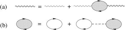
Figure 12: Dyson’s equation for the phonon propagator (a) where the Coulomb interactions are taken into account within the RPA (b).

The simplest approximation (beyond mean-field) which includes the Coulomb repulsion is the RPA shown in Fig. 12 (see e.g. Refs. Schrieffer64, ; Levin74, ), Eq. (14) now becomes for a one-band system

$$\left(\Omega_{q\mu}\right)^{2}=\left(\Omega_{q\mu}^{0}\right)^{2}+2\Omega^{0}_{q\mu}\frac{\Pi_{\mu}(q,\Omega_{q\mu})}{1-V(q)\chi_{0}(q,\Omega_{q\mu})}$$ (32)

where $\Pi_{\mu}(q,\Omega_{q\mu})=|g_{q\mu}|^{2}\chi_{0}(q,\Omega_{q\mu})$. We immediately see that including the Coulomb interaction can suppress the CDW instability. The second term in Eq. (32) no longer diverges when $q=2k_{F}$ and the softening of the $2k_{F}$ phonons occurs only for $\mu_{{\rm CDW}}<\lambda_{{\rm CDW},\mu}$, where

$$\mu_{{\rm CDW}}\equiv\frac{1}{2}\nu(0)V_{q=2k_{F}}.$$ (33)

From equation (32) we also find how the Coulomb interaction modifies the Peierls transition temperature

$$T_{{\rm CDW},\mu}=4\varepsilon_{{\rm F}}\exp\left(-\frac{1}{[\lambda_{{\rm CDW},\mu}-\mu_{{\rm CDW}}]}\right).$$ (34)

We will now estimate the magnitude of $\mu_{\rm CDW}$ from this residual Coulomb interaction for the (5,0) which was seen above to be the most unstable toward the formation of a CDW from distortion of the out-of-plane optical mode shown in Fig. 6. Carrying through the straightforward generalization of the RPA analysis for the multiple-band system, and carrying out the integrals in Eq. (31) for the Coulomb backward scattering interaction, we obtain $\mu_{\rm CDW}=0.24$. Note that this is quite close to $\lambda_{\rm CDW}=0.26$ for this particular instability. This indicates that it is possible that the Coulomb interaction can significantly suppress the CDW transition temperature or even remove the CDW instability altogether. Indeed, taking these values we find that $T_{\rm CDW}$ is suppressed to less than $10^{-18}$ K.

For the (6,0) CNT, we calculate the smaller value $\mu_{\rm CDW}=0.0019$. This will not change the value of $T_{\rm CDW}=5.0$ K that we calculated previously for the (6,0) CNT.

V.3 Phonon vertex renormalization through screening

It can be seen that the Coulomb interaction further can screen the electron-phonon vertex. By including screening through the RPA, we find that the screened vertex is given by Schrieffer64

$$\bar{g}_{q\mu}=\frac{g_{q\mu}}{1-V_{q}\chi_{0}(q)}$$ (35)

for a one-band system where $\chi_{0}(q)\equiv\chi_{0}(q,\Omega_{q\mu}=0)$. Thus we see that the inclusion of screening reduces the electron-phonon vertex. We note that in the treatment in Sec. V.2 of the CDW instability it would be inappropriate to use the screened vertices since this would lead to double-counting.

Full charge self-consistent calculations will determine the dressed electron-phonon vertex (see Appendices A and D). This is desirable in 3d, where the renormalization is presumably small. However in 1d, one would calculate greatly suppressed values for the couplings, dominated by the screening due to the logarithmic divergence of the susceptibility at $2k_{F}$. Because of the subtle interplay between these divergences, it is desirable to calculate the bare vertex and then manually put in the Coulomb interaction as we do.

Since with the method we use, the charge distribution is not calculated self-consistently, we calculate the bare electron-phonon vertex $g_{q\mu}$. We point out, however, that there is an approximation here. The true bare electron-phonon vertex should be calculated in the absence of the conduction electron entirely which is separately accounted for in the residual Coulomb term. In our method, however, the conduction electron is taken to adiabatically follow the ion through the distortion. Because of this, we expect our results to slightly underestimate the bare electron-phonon coupling vertices.

V.4 Modification of superconducting instability due to Coulomb interactions

To include the Coulomb interaction in the Eliashberg equations, it is necessary to dress both electron-phonon vertices shown in Fig. 14 according to Sec. V.3 as well as the phonon propagator according to Sec. V.2. This leads to the modified phonon-mediated interaction between electrons of

$$|\bar{g}_{q\mu}|^{2}D_{\mu}(q,\Omega) = \frac{|g_{q\mu}|^{2}}{(1-V_{q}\chi_{0}(q))^{2}}$$

$$\times \frac{2\Omega_{q\mu}^{0}}{\Omega^{2}-(\Omega_{q\mu}^{0})^{2}-2\Omega_{q\mu}^{0}|g_{q\mu}|^{2}\frac{\chi_{0}(q)}{1-V_{q}\chi_{0}(q)}}.$$

Using this leads to a modified result for the superconducting coupling constant $\lambda_{\rm SC}$. For a specific process of wave vector $q$, coupling points on the Fermi surface, we find that the renormalized contribution to the superconducting coupling constant is given by

$$\lambda_{q\mu}=\left(\frac{1}{(1-V_{q}\chi_{0}(q))^{2}}\right)\left(\frac{1}{1+\frac{2|g_{q\mu}|^{2}}{\Omega_{q\mu}^{0}}\frac{\chi_{0}(q)}{1-V_{q}\chi_{0}(q)}}\right)\lambda_{q\mu}^{0}$$ (37)

where $\lambda_{q\mu}^{0}$ is the unrenormalized contribution. All such contributions must be summed over to determine the total $\lambda_{\rm SC}$. The first and second factors tend to decrease and increase the electron-phonon coupling respectively. Physically, the first factor is due the screening of the electron-ion interaction due to conduction electrons. The second factor is due to the softening of particular modes due to the Kohn Anomaly which will in turn enhance the overall electron-phonon coupling. Since these renormalization factors depend on temperature through the susceptibility $\chi_{0}$, $T_{\rm SC}$ must be determined self-consistently.

In addition to the renormalization of the Coulomb vertex, there is also the direct Coulomb repulsion between electrons that is taken into account through the Coulomb pseudopotential $\mu^{*}_{\rm SC}$ which is included in McMillan’s expression McMillan68 ; Allen82

$$T_{\rm SC}=\frac{\langle\Omega\rangle}{1.2}\exp\left(-\frac{1.04(1+\lambda_{\rm SC})}{[\lambda_{{\rm SC}}-\mu^{*}_{{\rm SC}}(1+0.62\lambda_{\rm SC})]}\right)$$ (38)

where

$$\mu^{*}_{{\rm SC}}=\frac{\mu_{{\rm SC}}}{1+\mu_{{\rm SC}}\ln\left(\frac{E_{F}}{\omega_{D}}\right)}$$ (39)

and $\mu_{\rm SC}$ is the screened Coulomb interaction averaged over the Fermi surface.

We will now estimate $\mu^{*}_{\rm SC}$. Taking into account screening within the RPA one finds

$$V^{s}_{q}=\frac{V_{q}}{1-V_{q}\chi_{0}(q)}$$ (40)

for the screened Coulomb interaction. In 1d for $q\approx 2k_{F}$, $V^{s}_{q}\approx 0$. This is due to the divergence of $\chi_{0}(q)$ at $q=2k_{F}$. Also, one finds that for $q\approx 0$, $V^{s}(q)\approx 1/\nu(0)$. Using this RPA screened Coulomb interaction we find for our three band system of the (5,0) CNT

$$\mu_{\rm SC}\equiv\frac{1}{\nu_{\sigma}(0)}\sum_{k\tau k^{\prime}\tau^{\prime}}\delta(\varepsilon_{k\tau})\delta(\varepsilon_{k^{\prime}\tau^{\prime}})V_{\tau\tau^{\prime}}^{s}(k-k^{\prime})=0.25.$$ (41)

Then, using Eq. (39), we obtain $\mu_{\rm SC}^{*}=0.19$ for the Coulomb pseudopotential with the calculated values of the Fermi energy and Debye frequency.

We now see how taking into account the Coulomb interaction in this manner modifies the superconducting transition temperature for the (5,0) CNT. The most significant renormalization of the total superconducting $\lambda_{\rm SC}$ given by Eq. (37) will be for the $2k_{F}$ process that couples to the out-of-plane optical mode which was previously seen to have the overall strongest coupling. That is, at temperatures where the renormalized $\lambda_{\rm SC}$ will start to differ from the bare $\lambda_{\rm SC}^{0}$, all of the renormalization will come from this mode. Using Eqns. (37) and 38, we find that a self-consistent solution for the superconducting transition temperature occurs at $T_{\rm SC}\approx 1.1$ K which is larger than the previously calculated CDW transition temperature. This therefore shows that the Coulomb interactions can favor superconductivity over the CDW instability.

For the (6,0) CNT, we see that the value of $T_{\rm SC}$ without the inclusion Coulomb interaction is smaller than $T_{\rm CDW}=5$K that we computed in the previous section with the inclusion of the Coulomb interaction. We therefore conclude that the CDW will be dominant for the (6,0) CNT.

V.5 Summary of Coulomb effects

In the above, we have shown that the introduction of the residual Coulomb interaction will lower both the SC and CDW transition temperatures. We also illustrated the possibility that the CDW instability can be suppressed so much by Coulomb interactions that SC will be dominant at low temperatures. However, we stress the difficulty of obtaining such quantitative results. In principle, to obtain an accurate Coulomb interaction in our basis of Bloch states, one needs to use the interaction

$$V_{kk^{\prime}k^{\prime\prime}k^{\prime\prime\prime}}=\frac{1}{\kappa}\int d^{3}rd^{3}r^{\prime}\psi_{k}^{*}(\textbf{r})\psi_{k^{\prime}}^{*}(\textbf{r}^{\prime})\frac{e^{2}}{|\textbf{r}-\textbf{r}^{\prime}|}\psi_{k^{\prime\prime}}(\textbf{r}^{\prime})\psi_{k^{\prime\prime\prime}}(\textbf{r})$$ (42)

where the $\psi_{k}$’s are Bloch state wave functions of the CNT which is difficult to obtain. The Coulomb interaction $V_{q}$ we used is only a rough approximation to this more realistic interaction. On the other hand, the SC and CDW transition temperatures have exponential dependence on the Coulomb interaction parameters. One also has to be very careful not to double-count the electron-electron interaction terms taken into account in the single-particle energies $\varepsilon_{k}$ through the Hartree term. As shown in Appendix D, using a method in which the charge density is calculated self-consistently will give more accurate values for the phonon frequencies calculated through the FPA. However, there are serious difficulties with calculating the bare electron-phonon vertex with such a method as discussed in Sec. V.3.

VI DISCUSSION

VI.1 Comparison to other carbon based materials

As a consistency check, we now compare our results for the attractive potential due to electron-phonon coupling to established results for other carbon based solids, namely the intercalated graphene KC₈ and the carbon fullerene K₃C₆₀. Calculations of the density of states at the Fermi energy yield $\nu(0)=$ 0.24 (Ref. [Inoshita77, ]) and 0.29 (Ref. [Antropov92, ]) states/ eV / C atom for KC₈ and K₃C₆₀ respectively. Estimates of $\lambda_{\rm SC}$ for these are 0.21 (Ref. [Inoshita77, ]) and 0.7 (Ref. [Benedict95, ]). In the BCS theory, $\lambda_{\rm SC}$ is expressed in terms of the product of the electronic density of states at the Fermi level and the attractive pairing potential strength $\lambda_{\rm SC}=\nu(0)V$. Schrieffer64 Now that we have the magnitude $\lambda_{\rm SC}$ and $\nu(0)$, we can extract the magnitude of the pairing potential for the intercalated graphene, the fullerene, and the CNTs we study. The results are summarized in Table 6.

	KC8	K3C60	(5,0) CNT	(6,0) CNT	(5,5) CNT
$\nu(0)$ (eV-1)	0.24a	0.29b	0.16	0.068	0.034
$\lambda_{\rm SC}$	0.21a	0.7c	0.57	0.12	0.031
$V$ (eV)	0.875	2.4	3.6	1.8	0.92

Table 6: Density of states at the Fermi energy, the superconducting coupling strength, and the attractive potential strength for various carbon materials. Superscripts $a,b,$ and $c$ denote Refs. [Inoshita77, ], [Antropov92, ], and [Benedict95, ] respectively.

The following analysis will be very similar to that of Benedict et al. in Ref. Benedict95, The central idea in their analysis is as follows. Since curvature increases the amount of hybridization between $\sigma$ and $\pi$ states at the Fermi energy, the strict selection rules for phonon scattering between pure $\pi$ states in graphene will be lifted. The amount of $\sigma-\pi$ hybridization has roughly a $1/R$ dependence on the radius of curvature, so the matrix elements and therefore the attractive potential due to curvature will go as $1/R^{2}$.

Neglecting presence of pentagons in fullerenes, we write the attractive potential for the fullerene $V_{\rm{ball}}$ as the sum of contributions from that of the graphene sheet $V_{\rm{flat}}$ and that from curvature effects $V_{\rm{curve}}$

$$V_{\rm{ball}}=V_{\rm{flat}}+V_{\rm{curve}}.$$ (43)

This relation enables us to obtain the value for $V_{\rm{curve}}=1.5$ eV. Now we can write the expected attractive interaction for the CNT

$$V_{\rm{tube}}(R)=V_{\rm{flat}}+V_{\rm{curve}}\left(\frac{R_{0}/2}{R}\right)^{2}$$ (44)

where $R_{0}\approx 5$ Å is the radius of a fullerene and the factor of two comes in because there is twice as much $\sigma-\pi$ hybridization in a fullerene as there is in a CNT of radius $R_{0}$. Benedict95 In Fig. 13, we show that Eq. (44), which was calibrated by using only quantities from intercalated graphene and fullerenes, is consistent with the attractive potentials we obtain for the (5,0), (6,0), and (5,5) CNTs.

Figure 13: $V_{\rm tube}(R)$ from Eq. (44) calibrated with parameters from intercalated graphene and fullerenes (solid line) compared to the attractive potentials calculated for the representative CNTs (filled circles).

VI.2 Beyond Mean Field Theory

One-dimensional electron-phonon systems have several competing instabilities and the true ground state may be found only by analyzing their interplay. Voit87 ; Voit88 Hence, one may be concerned that we use a mean-field approach to analyze a 1d CNT. We point out that when we calculate the superconducting $T_{\rm SC}$ we include the interplay of the CDW and SC orders. That is, the effective superconducting coupling $\lambda_{\rm SC}$ that we obtain in Eq. 37 includes softening of the $2k_{F}$ phonon mode. Such an approach is equivalent to the two parameter RG analysis used in Ref. Grest76, . The mean-field transition temperature obtained by our method is equivalent to the coupling constants becoming of the order of unity in the RG analysis. At $T_{\rm SC}$ electrons start to pair, but the system has strong fluctuations in the phase of the SC order parameter. The most important kind of fluctuations are thermally activated phase slips, discussed originally for superconducting wires in Refs. Langer67, ; McCumber70, . Phase slips lead to only a gradual decrease of resistivity with temperatures below $T_{\rm SC}$.

For an incommensurate CDW, long range order may not appear at finite temperature either. To understand the physical meaning of the mean-field transition, we can introduce a Landau-Ginzburg formalism. caron94 Here we concentrate on the (5,0) and (6,0) CNTs which have three partially filled bands with Fermi points $k_{F}^{A}$ and $k_{F}^{B}$ where the exact relation $2k_{F}^{A}=k_{F}^{B}$ is satisfied. We introduce a complex order parameter $\Psi_{1}(x)$ related to the amplitude of the lattice distortion as $q(x)=e^{2ik^{A}_{F}x}\,\Psi_{1}(x)+e^{-2ik^{A}_{F}x}\,\Psi^{*}_{1}(x)$. At low temperature the free energy is given by $F_{\sigma}[\Psi_{1}]=\int dx(a|\Psi_{1}|^{2}+b|\Psi_{1}|^{4}+c|\frac{d\Psi_{1}}{dx}|^{2}).$ Below the mean-field transition temperature $T_{\rm CDW}$ we have $a<0$ and the system develops an amplitude for the order parameter $\Psi_{1}$. The phase of $\Psi_{1}$, however, is still fluctuating, leading to short range correlations for the CDW order $\langle\Psi_{1}(x)\Psi^{*}_{1}(0)\rangle\propto e^{-x/\xi(T)}$. Even at $T=0$ we can have at best a quasi long-range order for $\Psi_{1}$ due to the incommensurate value of $2k^{A}_{F}$. Lattice distortions at $2k^{B}_{F}$ can be included by introducing another complex field $\Psi_{2}(x)$ that contributes $e^{2ik^{B}_{F}x}\,\Psi_{2}(x)+e^{-2ik^{B}_{F}x}\,\Psi^{*}_{2}(x)$ to the distortion amplitude. The relation $2k^{A}_{F}=k^{B}_{F}$ implies that the free energy allows coupling between $\Psi_{1}$ and $\Psi_{2}$ of the form $F_{\pi\sigma}[\Psi_{1},\Psi_{2}]=\gamma\int dx(\Psi^{2}_{1}\Psi^{*}_{2}+\Psi^{*2}_{1}\Psi_{2})$, so when the amplitude of $\Psi_{1}$ is established, it will immediately induce the amplitude for $\Psi_{2}$ (although none of the fields have a long-range order). Appearance of such amplitudes should lead to a pseudogap state of the system below $T_{\rm CDW}$. caron94 The dominant contribution to electrical conductivity in a clean system would then come from the Goldstone mode of the phase of the $\Psi$’s, i.e. sliding of CDWs (Frölich mode). Any kind of disorder (e.g. impurities or crystal defects), however, gives strong pinning of the CDW phase and suppresses collective mode contributions to transport. Therefore, we expect insulating behavior of the low temperature resistivity in most experimentally relevant circumstances if CDW is the dominant low temperature phase.

VI.3 Experimental Implications

Proximity inducedKasumov99 ; Morpurgo99 as well as intrinsic Kociak01 ; Tang01 superconductivity has been experimentally observed in carbon nanotubes. On the other hand, the CDW state, despite being endemic to quasi 1d systems has never been reported for carbon nanotubes. As we discuss above, one needs to have very small carbon nanotubes to have electron-phonon interaction strong enough to make either the CDW or the SC instabilities appear at experimentally relevant temperatures. In this work we address quantitatively both of these instabilities. Our main conclusion is that when we include Coulomb interaction between electrons, the CDW instability does no appear even for the ultrasmall nanotubes, whereas the superconducting $T_{\rm SC}$ may be in the few Kelvin range.

In the work by Kociak et al. in Ref. Kociak01, , electronic transport through ropes of single-walled CNTs suspended between normal metal contacts was measured. The ropes are composed of several hundred CNTs in parallel with diameters of the order 1.4 nm. It was found that below 0.5 K, the resistance abruptly drops, an effect which is destroyed by the application of an external magnetic field of order 1 T. The largest radius CNT we study is the (5,5) CNT, which was seen to be in the regime where zone-folding is applicable. For this CNT, we calculated $\lambda_{\rm SC}=0.031$, a value far too small to support superconductivity at this temperature even without the inclusion of the Coulomb interaction. This small value of $\lambda_{\rm SC}$ is consistent with the experimental measurements of the electron-phonon coupling in CNTs of similar diameter by Hertel et al. in Ref. Hertel00, . It is possible that the interactions between CNTs in the rope play a tantamount role for superconductivity in the experiment of Ref. Kociak01, as suggested by Gonzalez in Ref. Gonzalez02, . Another possibility is that a small number of nanotubes in the rope have a small diameter. For nanotubes with a diameter of 4 Å we find superconducting $T_{\rm SC}$ in the 1 K range which would be consistent with these experiments. A small number of superconducting nanotubes could provide a short-circuiting in transport measurements or even induce superconductivity in other CNTs via the proximity effect.

In the experimental work of Tang et al. in Ref. Tang01, , electrical transport was measured through a zeolite matrix containing single-walled CNTs. In the zeolite matrix, the CNTs are well-separated from each other creating an idealized one-dimensional system. The diameters of the CNTs were determined to be approximately 4 Å by measuring the radial breathing phonon mode frequency by Raman spectroscopy. The superconducting transition temperature for this system was found to be 15 K from transport measurements. In addition, the Meissner effect was observed through the temperature dependence of the magnetic susceptibility suggesting that the large currents observed in transport measurements are not from the sliding charge-density wave collective mode, but are indeed from superconducting correlations.

The ultrasmall (5,0) CNT we study is the likely candidate structure for the CNTs confined in the zeolite matrix in these experiments. We find for this system that the electron-phonon coupling is very strong. We find in the mean-field theory, neglecting Coulomb interactions, that $T_{\rm CDW}=160$ K and $T_{\rm SC}=64$ K, indicating that the charge-density wave instability is stronger in this approximation. However, putting in the Coulomb interaction as in Eq. (28), the charge-density wave transition was suppressed to very low temperatures, making superconductivity dominant with $T_{\rm SC}=1$ K. Discrepancy between our calculated $T_{\rm SC}$ and the experimentally observed 15 K should not be a reason for concern. The superconducting transition temperature in Eq. 38 is exponentially sensitive to the strength of the Coulomb interaction, and our estimates of the latter are not very accurate.

VII Summary and Conclusions

In this work, we have used the Frölich Hamiltonian written in Eq. (1) to study three types of small-radius CNTs. For this Hamiltonian, the band structure energies were computed by using an empirical tight-binding method Mehl96 to first relax the structure, and then to compute the eigenvalues of the secular tight-binding equation. The electron-phonon interaction $g_{k\tau k^{\prime}\tau^{\prime}\mu}$ is evaluated for scattering between all Fermi points. The dressed phonon frequencies $\Omega_{q\mu}$ are computed by using the frozen-phonon approximation given in Eq. (8) by the displacement vectors from the dynamical matrix of graphene given in Ref. Jishi93, . The undressed frequencies $\Omega_{q\mu}^{0}$, which enter the Frölich Hamiltonian in Eq. (1), are then extracted by using the previously computed quantities of the band structure and the electron-phonon coupling, and the RPA analysis of the Peierls instability. This method is elaborated in Sec. II.4. After the calculation of these quantities, the effective Frölich Hamiltonian has been fully constructed. The remarkable agreement of the coefficients of the logarithmic divergences computed by using quantities from the band structure and the electron-phonon coupling with the frozen-phonon frequencies is a consistency check for this method.

With the Frölich Hamiltonian, we then used the RPA analysis of the Peierls instability (in Sec. IV.1 ) and the McMillan equation (in Sec. IV.2 and Appendix B) to obtain the charge-density wave and superconducting transition temperatures, the result with the higher transition temperature being the dominant phase at low temperatures. For instance, when the CDW is dominant, the Fermi surface will be destroyed around $T_{\rm CDW}$ eliminating superconductivity altogether. By this method, we provided an exhaustive analysis of three types of CNTs: (5,0), (6,0), and (5,5). The more conventional larger-radius (5,5) CNT was seen to be stable against the CDW and SC transitions down to very low temperatures ($\ll 1$K) if we only include electron-phonon interactions. For the ultrasmall radius (5,0) and (6,0) CNTs, however, the CDW was found to be the dominant phase, with transition temperatures of $160$ and $6$ K respectively. For both of these CNTs, $2k_{F}$ is incommensurate with the underlying lattice. Furthermore, in contrast to larger radius CNTs which have dominant electron-phonon coupling to the in-plane phonon modes, the ultrasmall (5,0) and (6,0) CNTs were found to have dominant coupling to the out-of-plane phonon modes (see Fig. 6), as seen from the direct computation of the electron-phonon matrix elements $M_{k\tau k^{\prime}\tau^{\prime}\mu}$. This is further supported by the frozen-phonon computation of frequencies which show the most robust Kohn anomalies for these modes (see Fig. 6).

When we include the Coulomb interaction, for the (5,0) CNT we find that the CDW order is suppressed much more strongly than superconductivity. More specifically, our analysis presented in Sec. V shows that the CDW transition is pushed down to unobservably low temperatures, whereas the superconducting $T_{\rm SC}$ is reduced to 1 K. Hence our calculation supports the possibility of observing superconductivity in ultrasmall CNTs. It is quite foreseeable that a more detailed model for the Coulomb interaction could raise $T_{\rm SC}$ to the value seen experimentally, especially considering the exponential dependence of the superconducting transition temperature on the Coulomb interaction strength. For the (6,0) CNT, we found that the CDW remains dominant when the Coulomb interactions are included due to the weak Coulomb interaction between electrons at the Fermi points, and occurs at around $T_{\rm CDW}=$5K.

Appendix A The electron-phonon coupling vertices

The electron-phonon coupling matrix is given by

$$M_{k\tau k^{\prime}\tau^{\prime}\mu}=N\langle{\psi_{k\tau}}|\sum_{i}\frac{\partial V}{\partial{\bf R}_{0i}}\cdot\hat{\epsilon}_{q\mu}(i)|{\psi_{k^{\prime}\tau^{\prime}}}\rangle.$$ (45)

One can see that the above expression can be evaluated by using the finite difference formula

$$M_{k\tau k^{\prime}\tau^{\prime}\mu}=\frac{1}{u}\langle{\psi_{k\tau}}|(V^{q\mu}-V_{0})|{\psi_{k^{\prime}\tau^{\prime}}}\rangle.$$ (46)

A method for calculating this expression with a plane-wave basis set was previously developed.Lam86 This section will be devoted to describing how to calculate $M_{k\tau k^{\prime}\tau^{\prime}\mu}$ with a tight-binding method. We introduce the standard tight-binding notation

$$|{\psi_{k\tau}}\rangle=\sum_{il}A_{k\tau il}|{\chi_{kil}}\rangle$$ (47)

$$|{\chi_{kil}}\rangle=\frac{1}{\sqrt{N}}\sum_{n}e^{ik\cdot R_{n}}|{\phi_{nil}}\rangle.$$ (48)

Here $n$ runs over unit cells and $i$ runs over basis vectors in the unit cell and $l$ over orbital type. Because the kinetic energy operator will be the same in the perturbed and unperturbed Hamiltonians, we can write

$$M_{k\tau k^{\prime}\tau^{\prime}\mu}=\frac{1}{u}\langle{\psi_{k\tau}}|(H^{q\mu}-\varepsilon_{F})|{\psi_{k^{\prime}\tau^{\prime}}}\rangle.$$ (49)

The reason why we keep the $\varepsilon_{F}$ term which clearly is zero through orthogonality will become clear below. Expanding the wave functions in the tight-binding basis set, we obtain

$$M_{k\tau k^{\prime}\tau^{\prime}\mu}=\frac{1}{u}\sum_{ili^{\prime}l^{\prime}}A^{*}_{k\tau il}\langle{\chi_{kil}}|(H^{q\mu}-\varepsilon_{F})|{\chi_{k^{\prime}i^{\prime}l^{\prime}}}\rangle A_{k^{\prime}\tau^{\prime}i^{\prime}l^{\prime}}.$$ (50)

Now, we write $|{\chi_{kil}^{q\mu}}\rangle=|{\chi_{kil}}\rangle+|{\delta\chi_{kil}^{q\mu}}\rangle$ where the orbitals of $|{\chi_{kil}^{q\mu}}\rangle$ are centered on the perturbed lattice. Inserting this into the above equation, we obtain

$$M_{k\tau k^{\prime}\tau^{\prime}\mu} = \frac{1}{u}\sum_{ili^{\prime}l^{\prime}}A^{*}_{k\tau il}\left(\langle{\chi_{kil}^{q\mu}}|(H^{q\mu}-\varepsilon_{F})|{\chi_{k^{\prime}i^{\prime}l^{\prime}}^{q\mu}}\rangle\right.$$

$$- \left.\left(\langle{\delta\chi_{kil}^{q\mu}}|(H^{q\mu}-\varepsilon_{F})|{\chi_{k^{\prime}i^{\prime}l^{\prime}}}\rangle+{\rm h.c.}\right)\right)A_{k^{\prime}\tau^{\prime}i^{\prime}l^{\prime}}.$$

In the second term we can do the substitution $H^{q\mu}\rightarrow H_{0}$ because the effect of doing this will be second order in $u$ and we are interested in an expression that is accurate to first order. Then, this term will be

$$\sum_{ili^{\prime}l^{\prime}}A^{*}_{k\tau il}\left(\langle{\delta\chi_{kil}}|(H-\varepsilon_{F})|{\chi_{k^{\prime}i^{\prime}l^{\prime}}}\rangle+h.c.\right)A_{k^{\prime}\tau^{\prime}i^{\prime}l^{\prime}}$$ (52)

$$= \sum_{il}A^{*}_{k\tau il}\langle{\delta\chi_{kil}}|(H-\varepsilon_{F})|{\psi_{k^{\prime}\tau^{\prime}}}\rangle+h.c.=0.$$

So we finally have the expression

$$M_{k\tau k^{\prime}\tau^{\prime}\mu}=\frac{1}{u}\sum_{ili^{\prime}l^{\prime}}A^{*}_{k\tau il}\langle{\chi_{kil}^{q\mu}}|(H^{q\mu}-\varepsilon_{F})|{\chi_{k^{\prime}i^{\prime}l^{\prime}}^{q\mu}}\rangle A_{k^{\prime}\tau^{\prime}i^{\prime}l^{\prime}}.$$ (53)

This expression can be computed by evaluating the tight-binding Hamiltonian and overlap matrices for the distorted lattice, evaluating the coefficients $A_{k\tau il}$ and $A_{k^{\prime}\tau^{\prime}i^{\prime}l^{\prime}}$ of the wave functions for the undistorted lattice, and performing the above sum. There is a slight technical problem with the above method because $k$ and $k^{\prime}$ are not the same in the tight-binding matrix. However, it can be shown that the correct result will be obtained by using $\langle{\chi_{kil}^{q\mu}}|H^{q\mu}|{\chi_{ki^{\prime}l^{\prime}}^{q\mu}}\rangle$ and $\langle\chi_{kil}^{q\mu}|{\chi_{ki^{\prime}l^{\prime}}^{q\mu}}\rangle$ for the tight-binding and overlap matrices (or the similar expression with $k\rightarrow k^{\prime}$) in the limit of a large supercell. That is, when the distance over which neighboring atoms interact is small compared to the length of a unit cell, this method becomes exact. When we apply this method, we checked for convergence of the coupling as a function of the unit cell size.

Appendix B Isotropic Eliashberg equations in 1D

Obtaining quantitative parameters of superconductors described by the BCS theory like the transition temperature and the wave vector-dependent superconducting gap from microscopic models has developed into a powerful tool for understanding experimentally realized systems as well as even predicting new superconductors.Cohen86 Though excellent review articles exist, Allen82 ; Rainer86 we will establish the key results of the theory below in attempt to be as self-contained as possible. We will also show how to incorporate the electron-phonon coupling into the phonon parameters which become important in 1d due to the CDW instability.

Figure 14: Migdal’s expression for the electronic self-energy. The thick line denotes the dressed electronic Green’s function and the wavy line denotes the phonon Green’s functions.

In the following to simplify notation, we will consider a single band system only. The central ingredient which, in principle, allows one to calculate the superconducting transition temperature to high accuracy is Migdal’s theorem Migdal58 which allows one to evaluate the electron self-energy with small error as

$${\bf\Sigma}(k,i\omega_{n})=-\frac{1}{\beta} \sum_{k^{\prime}n^{\prime}\mu} \tau_{3}{\bf G}(k^{\prime},i\omega_{n^{\prime}})\tau_{3}|g_{kk^{\prime}\mu}|^{2}$$ (54)

$$\times D_{0\mu}(k-k^{\prime},n-n^{\prime}).$$

This expression for the self-energy is shown in Fig. 14. In this equation, $\beta$ is inverse temperature, $\tau_{i}$ are Pauli matrices ($i=0$ gives the identity matrix while $i=1,2,3$ give the $x,y,z$ Pauli matrices respectively), $D_{0}$ is the noninteracting phonon Green’s function, and $\omega_{n}=\pi(2n+1)/\beta$ are the fermionic Matsubara frequencies. The electronic Nambu-Green’s function, a $2\times 2$ matrix, is given by $\bf G\mit(k,i\omega_{n})=(i\omega_{n}\tau_{0}-\varepsilon_{k}\tau_{3}-\bf\Sigma\mit)^{-1}$.

Now, we can expand $\bf\Sigma\mit$ in terms of Pauli matrices

$${\bf\Sigma}=(1-Z)i\omega_{n}\tau_{0}+\phi\tau_{1}.$$ (55)

We did not include the $\tau_{3}$ term because this just shifts the quasiparticle energies and similarly we neglected the $\tau_{2}$ term which can be eliminated by a proper choice of phase for $\phi$. Written in terms of these parameters, the Green’s function becomes

$${\bf G}=-\frac{Zi\omega_{n}\tau_{0}+\varepsilon_{k}\tau_{3}+\phi\tau_{1}}{(Z\omega_{n})^{2}+\varepsilon_{k}^{2}+\phi^{2}}.$$ (56)

Inserting this into 54 we obtain

$${\bf\Sigma} = \frac{1}{\beta}\sum_{k^{\prime}n^{\prime}\mu}\frac{Z^{\prime}i\omega_{n^{\prime}}\tau_{0}+\varepsilon_{k^{\prime}}\tau_{3}-\phi^{\prime}\tau_{1}}{(Z^{\prime}\omega_{n^{\prime}})^{2}+\varepsilon_{k^{\prime}}^{2}+\phi^{\prime 2}}$$ (57)

$$\times |g_{kk^{\prime}\mu}|^{2}D_{0\mu}(k-k^{\prime},n-n^{\prime}).$$

Now, we insert the identity $\int d\varepsilon\delta(\varepsilon-\varepsilon_{k}^{\prime})$ into the above expression to obtain

$${\bf\Sigma} = \frac{1}{\beta}\int d\varepsilon\sum_{k^{\prime}n^{\prime}\mu}\delta(\varepsilon-\varepsilon_{k})\frac{Z^{\prime}i\omega_{n^{\prime}}\tau_{0}+\varepsilon\tau_{3}-\phi^{\prime}\tau_{1}}{(Z^{\prime}\omega_{n^{\prime}})^{2}+\varepsilon^{2}+\phi^{\prime 2}}$$ (58)

$$\times |g_{kk^{\prime}\mu}|^{2}D_{0\mu}(k-k^{\prime},n-n^{\prime}).$$

The Lorentzian term in the integrand peaks very strongly at $\varepsilon=\varepsilon_{F}=0$ with width on the order of temperature. Assuming that the rest of the integrand doesn’t vary as rapidly about $\varepsilon=0$, we can replace $\delta(\varepsilon-\varepsilon_{k^{\prime}})$ with $\delta(\varepsilon_{k^{\prime}})$ and perform the $\varepsilon$ integral to obtain

$${\bf\Sigma}=\frac{\pi}{\beta}\sum_{k^{\prime}n^{\prime}\mu}\delta(\varepsilon_{k^{\prime}})\frac{Z^{\prime}i\omega_{n^{\prime}}\tau_{0}-\phi^{\prime}\tau_{1}}{\sqrt{(Z^{\prime}\omega_{n^{\prime}})^{2}+\phi^{\prime 2}}}|g_{kk^{\prime}\mu}|^{2}D_{0\mu}(k-k^{\prime},n-n^{\prime}).$$ (59)

This approximation can be seen to break down for small momentum (forward) scattering due to acoustic phonons. This case will be discussed in Appendix C. When close to $T_{\rm SC}$, $\phi^{\prime}$ will be small and can be neglected in the denominator of 59.

Now we perform the so-called isotropic approximation. Multiply both sides of 59 by $\delta(\varepsilon_{k})/\nu_{\sigma}(0)$ where $\nu_{\sigma}(0)$ is the density of states at the Fermi level per spin and sum over $k$. In the right-hand side of 59 we then replace $Z(k^{\prime},n^{\prime})$ and $\phi(k^{\prime},n^{\prime})$ with their Fermi-surface averages $Z_{n^{\prime}}$ and $\phi_{n^{\prime}}$. This approximation is valid when the Fermi-surface is fairly isotropic. Now by equating the coefficients of the matrices $\tau_{0}$ and $\tau_{1}$ we finally arrive at the equations

$$Z_{n}=1+f_{n}s_{n}\sum_{n^{\prime}}\lambda(n-n^{\prime})s_{n^{\prime}}$$ (60)

$$Z_{n}\Delta_{n}=\sum_{n^{\prime}}(\lambda(n-n^{\prime})-\mu_{\rm SC}^{*})f_{n^{\prime}}\Delta_{n^{\prime}}$$ (61)

where $f_{n}=1/|2n+1|$, $s_{n}={\rm sgn}(2n+1)$, $\Delta_{n}=\phi_{n}/Z_{n}$, and

$$\lambda(n-n^{\prime})=-\frac{1}{\nu_{\sigma}(0)}\sum_{kk^{\prime}\mu}\delta(\varepsilon_{k})\delta(\varepsilon_{k^{\prime}})|g_{kk^{\prime}\mu}|^{2}D_{0\mu}(k-k^{\prime},n-n^{\prime}).$$ (62)

The Coulomb pseudopotential $\mu_{\rm SC}^{*}$ was inserted to account for the bare electron-electron interaction that is not included in our original Hamiltonian Eq. (1). The superconducting transition temperature $T_{\rm SC}$ is the temperature at which nontrivial solutions for the gap $\Delta_{n}$ begin to appear. Equations (60), (61), and (62) are known as the isotropic Eliashberg equations.Eliashberg60 Input parameters have been calculated and the Eliashberg equations have been solved to calculate $T_{\rm SC}$ for a variety of superconductors described by the BCS theory. We also note that a generalization to the case where the Fermi surface is anisotropic is straightforward.Allen76

Now, for typical three-dimensional solids the phonon frequencies are affected very little by the electron-phonon coupling. Therefore, the above formalism where we have used the non-interacting phonon Green’s function $D_{0\mu}$ works remarkably well in 3d. This is not the case, however, in 1d where one is encountered with the CDW instability. A more accurate phonon Green’s function is given by

$$D_{\mu}(k,n)=\frac{2\Omega_{q\mu}^{0}}{(i\nu_{n})^{2}-(\Omega_{q\mu})^{2}}$$ (63)

where $\Omega_{q\mu}^{0}$ is the undressed frequency (without electron-phonon coupling) and $\Omega_{q\mu}$ is the dressed frequency (which, as seen above can have strong temperature dependence). Calculating the dressed phonon Green’s function can be challenging because one needs both $\Omega_{q\mu}^{0}$ and $\Omega_{q\mu}$. However, we notice that when we substitute Eq. (63) into Eq. (62) we have the fortuitous cancellation of $\Omega_{q\mu}^{0}$ in the numerator of $D_{\mu}(k,n)$ with that in the denominator of $|g_{kk^{\prime}\mu}|^{2}$. Thus one sees that knowledge of the undressed frequencies (which are significantly more difficult to obtain) will not be necessary to construct the Eliashberg equations. By doing the substitution $\Omega_{q}^{0}\rightarrow\Omega_{q\mu}$ in Eqns. (60), (61), and (62), one can thereby construct the “dressed” Eliashberg equations which takes into account the influence of the electron-phonon coupling on the phonon frequencies which is important in 1d.

Note also that since some modes will have temperature dependence, the Eliashberg equations must be solved self consistently. That is, we must find a temperature such that the SC transition temperature determined from the Eliashberg equations is the same as the temperature used for the input dressed phonon frequencies. This can be done by iteration. Furthermore, this method allows us to tell which will be the dominant phase at low temperature of our system. If we find a self-consistent solution of the Eliashberg equations and $T_{\rm SC}>T_{\rm CDW}$, then superconductivity will be the dominant correlation. Otherwise, the system will prefer the CDW state.

Finally, we will write down an expression which approximately solves the Eliashberg equations, originally developed by McMillan

$$T_{\rm SC}=\frac{\langle\Omega\rangle}{1.20}\exp\left[-\frac{1.04(1+\lambda_{\rm SC})}{\lambda_{\rm SC}-\mu_{\rm SC}^{*}(1+0.62\lambda_{\rm SC})}\right]$$ (64)

where $\lambda_{\rm SC}\equiv\lambda(0)$. From the above analysis, we see that to be self-consistent, one should use the dressed frequencies to evaluate $\lambda_{\rm SC}$.

Appendix C Incorporating $q\approx 0$ scattering from acoustic phonons in the Eliashberg equations.

In this Appendix, we discuss in detail the role of acoustic phonons for small-radius nanotubes. Earlier theoretical analysis of the electron-phonon interactions in 1d systems suggested that acoustic phonons can play a dominant role in stabilizing the superconducting state.Loss94 ; DeMartino03 We will show, however, that since the dominant coupling comes from optical modes, that this effect is not important for the CNTs we study.

We now consider explicitly the contributions to $q\approx 0$ scattering processes coupled to acoustic phonon modes which are not accounted for in the approximations leading to 59. For the electron-phonon coupling to acoustic modes, we take

$$|g_{q\mu}|^{2}=\frac{\gamma|q|/L}{1+(q/q_{0})^{2}}$$ (65)

where $q_{0}$ is a cut-off of order $k_{F}$ and $L$ is the system length. We also take $\Omega_{q\mu}=c|q|$ and $\varepsilon_{k}=v_{F}(|k|-k_{F})$. Inserting these quantities into 54, setting $Z=1$ for simplicity, we obtain for the off-diagonal element

$$\Delta_{n}^{(q\approx 0)} = \frac{1}{\beta}\sum_{n^{\prime}}\frac{1}{2\pi}\int dq\frac{\Delta_{n^{\prime}}}{\omega_{n^{\prime}}^{2}+(v_{F}q)^{2}}$$

$$\times \frac{\gamma|q|}{1+(q/q_{0})^{2}}\cdot\frac{2c|q|}{(\omega_{n}-\omega_{n^{\prime}})^{2}+(c|q|)^{2}}$$

This integral can be evaluated to give

$$\Delta_{n}^{(q\approx 0)} = \frac{\gamma}{v_{F}\beta}\sum_{n^{\prime}}\frac{\Delta_{n^{\prime}}}{|\omega_{n^{\prime}}|c+|\omega_{n}-\omega_{n^{\prime}}|v_{F}}$$

$$\times \frac{q_{0}}{|\omega_{n}-\omega_{n^{\prime}}|/c+q_{0}}\cdot\frac{q_{0}}{|\omega_{n}-\omega_{n^{\prime}}|/v_{F}+q_{0}}.$$

One then sees that scattering from $q\approx 0$ acoustic phonons gives an approximate contribution to $\lambda_{\rm SC}$ (when $n=n^{\prime}$) of $\lambda_{\rm SC}^{(q\approx 0)}={\gamma}/(\pi v_{F}c)$.

Now we consider the $q\approx 2k_{F}$ scattering process from the same acoustic phonon. For this process we obtain

$$\Delta_{n}^{(q\approx 2k_{F})}\approx\frac{1}{\beta}\sum_{n^{\prime}}|g_{q=2k_{F},\mu}|^{2}D(2k_{F},n-n^{\prime})$$

$$\times\frac{L}{2\pi}\int dq\frac{\Delta_{n^{\prime}}}{\omega_{n^{\prime}}^{2}+(v_{F}q)^{2}}.$$ (68)

This integral can be evaluated to give

$$\Delta_{n}^{(q\approx 2k_{F})}=\frac{4\gamma ck_{F}^{2}}{\beta v_{F}}\sum_{n^{\prime}}\frac{1}{(\omega_{n}-\omega_{n^{\prime}})^{2}+(c2k_{F})^{2}}\frac{1}{|\omega_{n^{\prime}}|}.$$ (69)

One then finds that this gives a contribution of $\lambda_{\rm SC}^{(q\approx 2k_{F})}=\gamma/(\pi v_{F}c)$ to $\lambda_{\rm SC}$ which is exactly the same as the $q\approx 0$ scattering contribution. Thus one sees that $q\approx 0$ scattering from acoustic phonons can be very important in one-dimensional electron-phonon systems. From such a process the so-called Wentzel-Bardeen instability Wentzel51 ; Bardeen51 ; Engelsberg64 can occur which has recently been studied in the context of CNTs.DeMartino03 We also note that a similar analysis can be carried out for the optical phonons, and it is found that the $q\approx 0$ processes are much smaller than the $q\approx 2k_{F}$ process.

With the above method, we now see how to include the contribution from $q\approx 0$ scattering into $\lambda_{\rm SC}$. To do this, we simply double the contributions to $\lambda_{\rm SC}$ from $2k_{F}$ processes which couple to acoustic phonons to include the $q\approx 0$ contribution. In practice, we find that using this procedure actually changes $\lambda_{\rm SC}$ by only a small amount. For instance, for the (5,0) CNT, $\lambda_{\rm SC}$ only increases by less than 1%. This is because the dominant contributions to $\lambda_{\rm SC}$ are from coupling to the optical modes as discussed in Sec. III.

We also point out that presence of the Wentzel-Bardeen singularity would significantly renormalize the acoustic phonon mode frequencies of the CNTs. The fact that the calculated phonon frequencies using the frozen-phonon approximation for the CNTs are quantitatively similar to the analogous modes of graphene as shown in Figs. 7, 9, and 11 further supports the the notion that the Wentzel-Bardeen instability is unimportant in these systems.

Appendix D Limitations of non self-consistent method

In this Appendix, we will discuss the limitations of using a method in which the charge density is not evaluated self-consistently. For simplicity, we will neglect the contribution from the exchange-correlation energy $E_{\rm XC}$ in the Kohn Sham energy functional.

First we will consider the case of the equilibrium lattice structure. For this, the self-consistent total energy is given by

$$E_{\rm SC}^{\rm eq} = \sum_{i}\langle{\psi_{i}}|\left(\frac{{\bf p}^{2}}{2m}+V_{\rm{ion}}^{\rm eq}({\bf r})+\frac{1}{2}\int d^{3}r^{\prime}\frac{n({\bf r}^{\prime})}{|{\bf r}-{\bf r}^{\prime}|}\right)|{\psi_{i}}\rangle$$ (70)

$$+ E_{\rm{ion-ion}}^{\rm eq}$$

where the charge-density is given by $n({\bf r})=\sum_{i}|\psi_{i}({\bf r})|^{2}$, $V_{\rm ion}^{\rm eq}$ is the ionic potential, and $E_{\rm ion-ion}^{\rm eq}$ is the ion-ion interaction. In the above and in what follows, the $i$ summation is carried out only over occupied electronic states. Applying the variational principle to Eq. 70 gives the equation for the wave functions $|{\psi_{i}}\rangle$ and therefore the charge-density $n({\bf r})$

$${\cal H}^{\rm eq}[n]|{\psi_{i}}\rangle=\varepsilon_{i}|{\psi_{i}}\rangle$$ (71)

where

$${\cal H}^{\rm eq}[n]=\frac{{\bf p}^{2}}{2m}+V_{\rm{ion}}({\bf r})+\int d^{3}r^{\prime}\frac{n({\bf r}^{\prime})}{|{\bf r}-{\bf r}^{\prime}|}.$$ (72)

In solving this equation, the charge density $n({\bf r})$ entering ${\cal H}^{\rm eq}[n]$ must be determined self-consistently to agree with the eigenfunctions $\psi_{i}$. Using this, the self-consistent totally energy for the equilibrium lattice is determined to be

$$E_{\rm SC}^{\rm eq}=\sum_{i}\langle{\psi_{i}}|{\cal H}^{\rm eq}[n]|{\psi_{i}}\rangle+F^{\rm eq}[n]$$ (73)

where

$$F^{\rm eq}[n]=-\frac{1}{2}\int d^{3}rd^{3}r^{\prime}\frac{n({\bf r})n({\bf r}^{\prime})}{|{\bf r}-{\bf r}^{\prime}|}+E_{\rm ion-ion}^{\rm eq}.$$ (74)

to be essentially the same as for non-interacting atoms. In the tight-binding limit we expect the equilibrium electron density to be essentially the same as for non-interacting atoms. If we denote the latter as $n_{0}({\bf r})$, we can replace $n({\bf r})$ by $n_{0}({\bf r})$ in $E_{\rm SC}^{\rm eq}$ and expect the resulting non-self-consistent total energy $E_{\rm NSC}^{\rm eq}$ to be quite close to the self-consistent total energy for the equilibrium lattice structure:

$$E_{\rm NSC}^{\rm eq}\approx E_{\rm SC}^{\rm eq}.$$ (75)

This approach is the basis for using an effective tight-binding model to calculate band structures.

Such a method, however, breaks down when we consider a lattice perturbed by a phonon. In the presence of a lattice distortion, the ionic potential changes to $V_{\rm ion}^{\rm dist}=V_{\rm ion}^{\rm eq}+\delta V_{\rm ion}$ which, in turn, makes the charge-density non-uniform $n=n_{0}+\delta n$. The energy of the distorted structure is then

$$E_{\rm SC}^{\rm dist} = \sum_{i}\langle{\psi_{i}}|\left(\frac{{\bf p}^{2}}{2m}+V_{\rm{ion}}^{\rm dist}({\bf r})+\frac{1}{2}\int d^{3}r^{\prime}\frac{n({\bf r}^{\prime})}{|{\bf r}-{\bf r}^{\prime}|}\right)|{\psi_{i}}\rangle$$ (76)

$$+ E_{\rm{ion-ion}}^{\rm dist}.$$

Now replacing $n$ with $n_{0}+\delta n$, this can be written as

$$E_{\rm SC}^{\rm dist} = \sum_{i}\langle{\psi_{i}}|{\cal H}^{\rm dist}[n_{0}]|{\psi_{i}}\rangle+F^{\rm dist}[n_{0}]$$

$$+ \frac{1}{2}\int d^{3}rd^{3}r^{\prime}\left(\frac{1}{|{\bf r}-{\bf r}^{\prime}|}\right)\delta n({\bf r})\delta n({\bf r^{\prime}})$$

where ${\cal H}^{\rm dist}$ and $F^{\rm dist}$ are given by ${\cal H}^{\rm eq}$ and $F^{\rm eq}$ defined above with $V_{\rm ion}^{\rm eq}$ and $E_{\rm ion-ion}^{\rm eq}$ replaced by $V_{\rm ion}^{\rm dist}$ and $E_{\rm ion-ion}^{\rm dist}$. The first two terms on the right of Eq. D can be seen to be the total energy of the distorted structure computed with the non-self-consistent method. We therefore obtain

$$E_{\rm SC}^{\rm dist}=E_{\rm NSC}^{\rm dist}+\frac{1}{2}\int d^{3}rd^{3}r^{\prime}\left(\frac{1}{|{\bf r}-{\bf r}^{\prime}|}\right)\delta n({\bf r})\delta n({\bf r^{\prime}}).$$ (78)

Subtracting Eq. 75 from this then gives

$$\Delta E_{\rm SC}=\Delta E_{\rm NSC}+\frac{1}{2}\int d^{3}rd^{3}r^{\prime}\left(\frac{1}{|{\bf r}-{\bf r}^{\prime}|}\right)\delta n({\bf r})\delta n({\bf r^{\prime}})$$ (79)

where $\Delta E_{\rm SC,NSC}=E_{\rm SC,NSC}^{\rm dist}-E_{\rm SC,NSC}^{\rm eq}$. Rewriting the second term in momentum space gives

$$\Delta E_{\rm SC}=\Delta E_{\rm NSC}+\frac{1}{2}\int\frac{d^{3}q}{(2\pi)^{3}}V(q)|\delta n_{\bf q}|^{2}.$$ (80)

which then makes it clear that $\Delta E_{\rm SC}>\Delta E_{\rm NSC}$. So we see that using the a non-self-consistent method to calculate phonon frequencies by the frozen-phonon approximation will underestimate the phonon frequencies. More specifically, in a non-self-consistent method, the Hartree term displayed in Eq. (80) is not accounted for. This should be particularly important in the vicinity of a CDW instability, where there will be a larger response of the charge distribution to a lattice distortion.

Appendix E Derivation of Eq. (31)

In this Appendix, we will derive Eq. (31) by evaluating the integral appearing in Eq. (V.1). To estimate this Coulomb interaction integral, we will take the tight-binding wave function of graphene

$$\psi_{{\bf k}\gamma}({\bf r})=\frac{1}{\sqrt{N}}\sum_{n}e^{i{\bf k}\cdot{\bf R}_{n}}\frac{1}{\sqrt{2}}\left(\gamma\frac{f({\bf k})}{|f({\bf k})|}\phi_{n1}({\bf r})+\phi_{n2}({\bf r})\right).$$ (81)

Now ${\bf k}$ is a two dimensional vector in reciprocal space of the graphene lattice and $\gamma=\pm 1$ corresponds to the conduction and valence bands. Orbitals centered on the first and second carbon atoms respectively in the $n$th unit cell are given by $\phi_{n1}({\bf r})$ and $\phi_{n2}({\bf r})$ respectively, and $f({\bf k})$ is given by $f({\bf k})=1+e^{-i{\bf k}\cdot{\bf a}_{1}}+e^{-i{\bf k}\cdot{\bf a}_{2}}$ where ${\bf a}_{1}$ and ${\bf a}_{2}$ are the lattice vectors of graphene. For metallic large radius CNTs, the Fermi points correspond to ${\bf K}=\frac{1}{3}({\bf b}_{1}-{\bf b}_{2})$ and ${\bf K}^{\prime}=\frac{2}{3}({\bf b}_{1}-{\bf b}_{2})$ where ${\bf b}_{1}$ and ${\bf b}_{2}$ are the reciprocal lattice vectors corresponding to ${\bf a}_{1}$ and ${\bf a}_{2}$. For these points, we have $f({\bf K})=f({\bf K}^{\prime})=0$. However, for the smaller radius CNTs we study, as indicated by the failure of the zone-folding method, the Fermi points are shifted away from ${\bf K}$ and ${\bf K}^{\prime}$. We denote the Fermi points of the inner band $\tau_{a}$ of the (5,0) CNT by ${\bf k}_{\tau_{a}+}={\bf K}+k_{x}{\bf\hat{x}}-k_{y}{\bf\hat{y}}$ and ${\bf k}_{\tau_{a}-}={\bf K}-k_{x}{\bf\hat{x}}-k_{y}{\bf\hat{y}}$ and for the other inner band $\tau_{b}$ by ${\bf k}_{\tau_{b}+}={\bf K}^{\prime}+k_{x}{\bf\hat{x}}+k_{y}{\bf\hat{y}}$ and ${\bf k}_{\tau_{b}-}={\bf K}^{\prime}-k_{x}{\bf\hat{x}}+k_{y}{\bf\hat{y}}$ where the $x$-direction is still along the CNT axis and the $y$-direction is along the perimeter.

For backward scattering, we take $q\approx 2k_{F},k\approx-k_{F},k^{\prime}\approx k_{F}$. Keeping only products of Carbon orbitals centered on the same atom, we obtain

$$\psi_{k+q\tau_{a}}^{*}({\bf r})\psi_{k\tau_{a}}({\bf r}) \approx \frac{1}{N}\sum_{n}e^{-iq{\bf\hat{x}}\cdot{\bf R}_{n}}\frac{1}{2}$$

$$\times \left(\frac{f^{*}({\bf k}_{\tau_{a}+})f({\bf k}_{\tau_{a}-})}{|f^{*}({\bf k}_{\tau_{a}+})f({\bf k}_{\tau_{a}-})|}|\phi_{n1}({\bf r})|^{2}\right.$$

$$+\left.|\phi_{n2}({\bf r})|^{2}\frac{}{}\right).$$

Now we make use of the slow variation of $e^{-iqx}$ compared to the localized orbitals to write

$$\psi_{k+q\tau}^{*}({\bf r})\psi_{k\tau}({\bf r}) \approx e^{-iqx}\frac{1}{N}\sum_{n}\frac{1}{2}$$

$$\times \left(\frac{f^{*}({\bf k}_{\tau_{a}+})f({\bf k}_{\tau_{a}-})}{|f^{*}({\bf k}_{\tau_{a}+})f({\bf k}_{\tau_{a}-})|}|\phi_{n1}({\bf r})|^{2}\right.$$

$$+\left.e^{iq{\bf\hat{x}}\cdot{\bf t}}|\phi_{n2}({\bf r})|^{2}\frac{}{}\right)$$

where ${\bf t}=\frac{1}{\sqrt{3}}a{\bf\hat{x}}$ is the basis vector for the second Carbon atom in the primitive unit cell. Finally, in evaluating the integral in Eq. (V.1) it is sufficient to replace the functions $\frac{1}{N}\sum_{n}|\phi_{n1,2}({\bf r})|^{2}$ which vary more rapidly than $V({\bf r})$ by their average values. That is, we substitute

$$\psi_{k+q\tau}^{*}({\bf r})\psi_{k\tau}({\bf r}) \rightarrow$$ (84)

$$\frac{1}{2\pi RL}e^{-iqx} \frac{1}{2} \left(\frac{f^{*}({\bf k}_{\tau_{a}+})f({\bf k}_{\tau_{a}-})}{|f^{*}({\bf k}_{\tau_{a}+})f({\bf k}_{\tau_{a}-})|}+e^{iq{\bf\hat{x}}\cdot{\bf t}}\right).$$

Using the same approximations for the factor $\psi_{k^{\prime}-q}({\bf r}^{\prime})\psi_{k^{\prime}}({\bf r}^{\prime})$, we obtain for the Coulomb interaction

$$V_{q\tau_{a}\tau_{a}} \approx \frac{1}{4}\left|\frac{f^{*}({\bf k}_{\tau_{a}+})f({\bf k}_{\tau_{a}-})}{|f^{*}({\bf k}_{\tau_{a}+})f({\bf k}_{\tau_{a}-})|}+e^{iq{\bf\hat{x}}\cdot{\bf t}}\right|^{2}$$

$$\times \frac{1}{L^{2}}\int dxdx^{\prime}e^{-iq(x-x^{\prime})}$$

$$\times \int_{0}^{2\pi R}\frac{dy}{2\pi R}\int_{0}^{2\pi R}\frac{dy^{\prime}}{2\pi R}V({\bf r}-{\bf r}^{\prime}).$$ (86)

We will now evaluate the prefactor in this equation for the inner band of the (5,0) and (6,0) CNTs. Using the calculated Fermi points along with the zone-folding method, we obtain $k_{x}=\pm\frac{0.11}{\sqrt{3}}\frac{2\pi}{a}$ and $k_{y}=\frac{1}{15}\frac{2\pi}{a}$ for the (5,0) CNT. From this we obtain

$$\frac{1}{4}\left|\frac{f^{*}({\bf k}_{\tau_{a}+})f({\bf k}_{\tau_{a}-})}{|f^{*}({\bf k}_{\tau_{a}+})f({\bf k}_{\tau_{a}-})|}+e^{iq{\bf\hat{x}}\cdot{\bf t}}\right|^{2}=0.59$$ (87)

For the (6,0) CNT the Fermi points are $k_{x}=\pm\frac{0.076}{\sqrt{3}}\frac{2\pi}{a}$ and $k_{y}=0$. This gives

$$\frac{1}{4}\left|\frac{f^{*}({\bf k}_{\tau_{a}+})f({\bf k}_{\tau_{a}-})}{|f^{*}({\bf k}_{\tau_{a}+})f({\bf k}_{\tau_{a}-})|}+e^{iq{\bf\hat{x}}\cdot{\bf t}}\right|^{2}=0.0016$$ (88)

which is smaller due to the different symmetry of the wavefunctions at the Fermi points. These are the values of the prefactor $\gamma$ appearing in Eq. (31).

References

- (1) S. Ijima, Nature 54, 56 (1991).
- (2) R. Egger, A. Bachtold, M. Fuhrer, and M. Bockrath, in R. Haug and H. Schoeller, eds., Interacting Electrons in Nanostructures (Springer Verlag, 2001).
- (3) M. Kociak, A. Y. Kasumov, S. Gueron, B. Reulet, I. I. Khodos, Y. B. Gorbatov, V. T. Volkov, L. Vaccarini, and H. Bouchiat, Phys. Rev. Lett. 86, 2416 (2001).
- (4) Z. Tang, L. Zhang, N. Wang, X. Zhang, G. Wen, G. Li, J. Wang, C. Chan, and P. Sheng, Science 292, 2462 (2001).
- (5) J. W. Mintmire, B. I. Dunlap, and C. T. White, Phys. Rev. Lett. 68, 631 (1992).
- (6) Y. Huang, M. Okada, K. Tanaka, and T. Yamabe, Solid State Commun. 97, 303 (1996).
- (7) A. Sedeki, L. G. Caron, and C. Bourbonnais, Phys. Rev. B 62, 6975 (2000).
- (8) O. Dubay, G. Kreese, and H. Kuzmany, Phys. Rev. Lett. 88, 235506 (2002).
- (9) L. X. Benedict, V. H. Crespi, S. G. Louie, and M. L. Cohen, Phys. Rev. B 52, 14935 (1995).
- (10) A. Sedeki, L. G. Caron, and C. Bourbonnais, Phys. Rev. B 65, 140515 (2002).
- (11) K. Byczuk (2002), eprint condmat/0206086.
- (12) J. Gonzalez, Phys. Rev. Lett. 88, 76403 (2002).
- (13) K. Kamide, T. Kimura, M. Nishida, and S. Kurihara (2003), eprint condmat/0301115.
- (14) J. R. Schrieffer, Theory of Superconductivity (Perseus Books, 1963).
- (15) R. Saito, G. Dresselhaus, and M. S. Dresselhaus, Physical Properties of Carbon Nanotubes (Imperial College Press, London, 1998).
- (16) M. J. Mehl and D. A. Papaconstantopoulos, Phys. Rev. B 54, 4519 (1996).
- (17) X. Blase, L. X. Benedict, E. L. Shirley, and S. G. Louie, Phys. Rev. Lett. 72, 1878 (1994).
- (18) W. Kohn, Phys. Rev. Lett. 2, 393 (1959).
- (19) R. E. Peierls, Quantum Theory of Solids (Oxford University, 1955).
- (20) K. Levin, D. L. Mills, and S. L. Cunningham, Phys. Rev. B 10, 3821 (1974).
- (21) R. Egger and A. O. Gogolin, Eur. Phys. J. B 3, 281 (1998).
- (22) P. Hohenberg and W. Kohn, Phys. Rev. 136, B864 (1964).
- (23) W. Kohn and L. Sham, Phys. Rev. 140, A1133 (1965).
- (24) P. Lam, M. Dacorogna, and M. Cohen, Phys. Rev. B 34, 5065 (1986).
- (25) R. A. Jishi, L. Venkataraman, M. S. Dresselhaus, and G. Dresselhaus, Chem. Phys. Lett. 209, 77 (1993).
- (26) M. T. Yin and M. L. Cohen, Phys. Rev. B 26, 5668 (1982).
- (27) L. M. Peng, Z. L. Zhang, Z. Q. Xue, Q. D. Wu, Z. N. Gu, and D. G. Pettifor, Phys. Rev. Lett. 85, 3249 (2000).
- (28) Z. M. Li, Z. K. Tang, H. J. Liu, N. Wang, C. T. Chan, R. Saito, S. Okada, G. D. Li, J. S. Chen, N. Nagasawa, et al., Phys. Rev. Lett. 87, 127401 (2001).
- (29) M. S. Dresselhaus and G. Dresselhaus, Adv. Phys. 30, 139 (1981).
- (30) A. Sedeki, L. G. Caron, and C. Bourbonnais, Phys. Rev. B 62, 6975 (2000).
- (31) A. J. Heeger, in J. T. Devreese, R. P. Evrard, and V. E. van Doren, eds., Highly Conducting One-Dimensional Solids (Plenum Press, New York, 1979).
- (32) V. L. Ginzburg and D. A. Kirzhnits, eds., High Temperature Superconductivity (The Consultants Bureau, New York, 1982).
- (33) W. L. McMillan, Phys. Rev. 167, 1967 (1967).
- (34) P. B. Allen and B. Mitrovic, in F. Seitz, D. Turnbull, and H. Ehrenreich, eds., Solid State Physics (Academic Press, New York, 1982), vol. 37.
- (35) G. Wentzel, Phys. Rev. 83, 168 (1951).
- (36) J. Bardeen, Rev. Mod. Phys. 23, 261 (1951).
- (37) S. Engelsberg and B. B. Varga, Phys. Rev. 136, A1582 (1964).
- (38) L. X. Benedict, V. H. Crespi, S. G. Louie, and M. L. Cohen, Phys. Rev. B 52, 8541 (1995).
- (39) T. Inoshita, K. Nakao, and H. Kamimura, J. Phys. Soc. Jpn. 43, 1237 (1977).
- (40) V. P. Antropov, O. Gunnarsson, and O. Jepsen, Phys. Rev. B 46, 13647 (1992).
- (41) J. Voit and H. J. Schulz, Phys. Rev. B 36, 968 (1987).
- (42) J. Voit and H. J. Schulz, Phys. Rev. B 37, 10068 (1988).
- (43) G. S. Grest, E. Abrahams, S.-T. Chui, P. A. Lee, and A. Zawadowski, Phys. Rev. B 14, 1225 (1976).
- (44) J. S. Langer and V. Ambegaokar, Phys. Rev. 164, 498 (1967).
- (45) D. E. McCumber and B. I. Halperin, Phys. Rev. B 1, 1054 (1970).
- (46) L. G. Caron, in J.-P. Farges, ed., Organic Conductors: Fundamentals and Applications (Marcel Dekker, New York, 1994).
- (47) A. Kasumov, R. Deblock, M. Kociak, B. Reulet, H. Bouchiat, I. Khodos, Y. Gorbatov, V. Volkov, C. Journet, , et al., Science 284, 1508 (1999).
- (48) A. Morpurgo, J. Kong, C. Marcus, and H. Dai, Science 286, 263 (1999).
- (49) T. Hertel and G. Moos, Phys. Rev. Lett. 84, 5002 (2000).
- (50) M. L. Cohen, Science 234, 549 (1986).
- (51) D. Rainer, Prog. in Low Temp. Phys. 10, 371 (1986).
- (52) A. B. Migdal, Zh. Eksp. Teor. Fiz. [Sov. Phys. JETP] 34, 1438 (1958).
- (53) G. M. Eliashberg, Zh. Eksp. Teor. Fiz. [Sov. Phys. JETP] 11, 696 (1960).
- (54) P. B. Allen, Phys. Rev. B 13, 1416 (1976).
- (55) D. Loss and T. Martin, Phys. Rev. B 50, 12160 (1994).
- (56) A. DeMartino and R. Egger, Phys. Rev. B 67, 235418 (2003).