Universality of Parametric Spectral Correlations: Local versus Extended Perturbing Potentials

Abstract

We explore the influence of an arbitrary external potential perturbation $V$ on the spectral properties of a weakly disordered conductor. In the framework of a statistical field theory of a nonlinear $\sigma$-model type we find, depending on the range and the profile of the external perturbation, two qualitatively different universal regimes of parametric spectral statistics (i.e. cross-correlations between the spectra of Hamiltonians $H$ and $H+V$). We identify the translational invariance of the correlations in the space of Hamiltonians as the key indicator of universality, and find the connection between the coordinate system in this space which makes the translational invariance manifest, and the physically measurable properties of the system. In particular, in the case of localized perturbations, the latter turn out to be the eigenphases of the scattering matrix for scattering off the perturbing potential $V$. They also have a purely statistical interpretation in terms of the moments of the level velocity distribution. Finally, on the basis of this analysis, a set of results obtained recently by the authors using random matrix theory methods is shown to be applicable to a much wider class of disordered and chaotic structures.

I Introduction

The statistical approach to the study of the quantum spectra of complex Hamiltonians $H$ was pioneered in the 1950’s in connection with the study of resonances in nuclear scattering wigner ; dyson_a . The approach was formalized by Dyson dyson_a , who identified three universal types of spectral statistics as determined by the symmetry properties of the corresponding ensembles of random Hamiltonians. The theory of Wigner and Dyson, together with its extensions, is usually referred to as random matrix theory (RMT). Within RMT, spectral correlations of each type (symmetry class) of statistics are described by the corresponding set of universal functions, once the energies are rescaled by the average level spacing $\bar{\Delta}$. The latter is the only non-universal parameter of the theory, where non-universality implies dependence on the specifics (other than the symmetry class) of the distribution functions defining the Hamiltonian ensemble. The symmetry classes are labeled by the index $\beta$ which takes the values $\beta=1$ for real (time-invariant) Hamiltonians (so-called orthogonal class), $\beta=2$ for complex Hamiltonians (unitary class), and $\beta=4$ for Hamiltonians with broken spin-rotation symmetry (symplectic class).

For example, in the unitary class ($\beta=2$), the normalized two-point correlation function of the density of states (DoS), $\nu(\varepsilon)=\operatorname{tr}\delta(\varepsilon-H)$,

$$R_{2}(\Omega)=\bar{\Delta}^{2}\langle\nu(\varepsilon+\Omega/2)\nu(\varepsilon-\Omega/2)\rangle$$ (1)

can be expressed as

$$R_{2}(s)=1+\displaystyle\frac{1}{2}\mathrm{Re}\int_{1}^{\infty}d\lambda_{1}\int_{-1}^{1}d\lambda\;e^{i\pi s_{+}(\lambda_{1}-\lambda)}\\ =\delta(s)+1-k^{2}(s)\;,$$ (2)

where

$$k(s)=\displaystyle\frac{\sin(\pi s)}{\pi s}\;,$$ (3)

$s=\Omega/\bar{\Delta}$, and where $s_{+}=s+i0$. The delta function in (2) represents the autocorrelation of an energy level with itself; the constant term is the disconnected contribution, and the oscillating term corresponds to non-trivial correlations between different levels. Similar, although slightly more convoluted, expressions are well known for other symmetry classes.

As became clear in the subsequent development of the theory, Wigner-Dyson statistics possesses a remarkable universality: beyond the manifestly model constructions of RMT, Wigner-Dyson statistics occurs both in quantum weakly disordered systems efetov_p ; efetov $H=H_{0}+H_{\text{dis}}$, where the statistical description follows naturally from the ensemble of realizations of the disordered part of the Hamiltonian $H_{\text{dis}}$, as well as in individual classically chaotic Hamiltonians bohigas_giannoni upon averaging over a sufficiently wide spectral window. The status of the last two statements is somewhat different: while the former has been rigorously established efetov_p ; efetov , the latter statement is known as the Bohigas-Giannoni-Schmit (BGS) bohigas_giannoni conjecture. Crucially, the existence of a statistical ensemble allows average properties of the disordered Hamiltonian to be formulated in the framework of a quantum field theory of nonlinear sigma model type (NL$\sigma$M) valid in the limit $g\gg 1$. Here, the dimensionless conductance $g$ denotes a non-universal parameter which depends on the deterministic part of the Hamiltonian $H_{0}$ – and through it on the sample geometry – as well as on details of the distribution of $H_{\text{dis}}$. By contrast, properties of an individual system are much less amenable to treatment by means of a statistical field theory and, despite recent encouraging progress andreev_agam_simons , a convincing formal proof of the BGS conjecture is lacking. The existence of a proof of Wigner-Dyson statistics in quantum disordered systems generates a dichotomy of approaches: if universality is assumed or established by other means, RMT calculations can be employed to obtain specific answers. On the other hand, NL$\sigma$M calculations often represent the only available route to establish universality and to explore deviations from it (typically as expansions in $1/g$).

A corollary of the above universality is the fact that, apart form a possible modification of the average DoS $\bar{\Delta}^{-1}$, the spectral statistics of $H=H_{0}+H_{\text{dis}}$ and $H_{V}=H_{0}+H_{\text{dis}}+V$ are indistinguishable zee unless $V$ is so large that $H_{0}+H_{\text{dis}}$ generate only perturbative corrections to its eigenvalues (the same condition, of course, applies to the relation between $H_{0}$ and $H_{\text{dis}}$). Such universality dictates that the statistics of spectral lines tracing the evolution of eigenvalues as functions of a coordinate $X$ along a typical curve in the Hamiltonian space connecting $H_{0}$ to $H_{0}+V$ must possess some kind of stationarity dyson_b . This stationarity is reflected, in turn, in the universality of parametric spectral correlations parametric (i.e. cross-correlations between the spectra of $H$ and $H_{V}$ averaged over the realizations of $H_{\text{dis}}$). Indeed, as first pointed out in Refs. simons_altshuler ; szafer ; altshuler_simons , for a broad class of $V$’s the parametric spectral correlators are expressed via another set of universal functions (again determined only by the symmetry of the Hamiltonian ensemble) which depend, in addition to the level density, on a single extra non-universal parameter – the dispersion $C(0)$ of the distribution of level velocities $\bar{\Delta}^{-1}\partial\varepsilon_{i}/\partial X\equiv\bar{\Delta}^{-1}\partial_{X}\varepsilon_{i}$, where $\varepsilon_{i}$ is a typical eigenlevel of $H$. (The use of the notation $C(0)$ for the dispersion of the distribution of level velocities is explained by the fact that it is the limiting value of the level velocity correlation function $C(X)=\bar{\Delta}^{-2}\langle\partial_{\bar{X}}\varepsilon_{i}(\bar{X})\partial_{\bar{X}}\varepsilon_{i}(\bar{X}+X)\rangle$ simons_altshuler ; szafer ; altshuler_simons .) If the curve is a ‘straight line’ $H+XV$, the rescaled parameter

$$x_{0}=X\sqrt{C(0)}$$ (4)

is an effective measure of the strength of $XV$. Eq. (4) is, in essence, a relation between two phenomenological parameters, $x_{0}$ and $C(0)$. It is supplemented by a ‘microscopic’ definition of $x_{0}$ in terms of $XV$ simons_altshuler ; altshuler_simons

$$x_{0}^{2}=\displaystyle\frac{8}{\bar{\Delta}^{2}}X^{2}\langle\langle V\Pi V\rangle\rangle\;,$$ (5)

where the double angle brackets denote the matrix element of $\Pi$ on the vector space spanned by $V$, and the definition of the (non-universal) operator $\Pi$ strongly depends on $H_{0}$ and the distribution of $H_{\text{dis}}$. In a disordered metal, $\Pi$ becomes a resolvent of the diffusion operator simons_altshuler ; altshuler_simons , and, if $V$ is diagonal in the coordinate representation, the matrix element simplifies to $\langle\langle V\Pi V\rangle\rangle=L^{-2d}\int d{\mathbf{r}}d{\mathbf{r}}^{\prime}V({\mathbf{r}})\Pi({\mathbf{r}},{\mathbf{r}}^{\prime})V({\mathbf{r}}^{\prime})$, where $\Pi({\mathbf{r}},{\mathbf{r}}^{\prime})$ is the matrix element of $\Pi$ in the coordinate basis, $L$ is the linear size of the sample, and $d$ are the space dimensions. The parameter $x_{0}$ can be thought of as a scalar norm (in the space of Hamiltonians) of the ‘distance’ between $H$ and $H+XV$, and Eq. (5) can correspondingly be viewed as fixing a particular prescription for the norm.

The importance of Eq. (4) is underscored by the fact that in practice, measuring $V$ directly is often impossible or very difficult, and the Green function of the diffusion operator is itself a complicated object in an irregularly shaped sample. Consequently, direct evaluation of (5) is seldom feasible. On the other hand, collecting statistics on level velocities is relatively straightforward, so that Eq. (4) is the only link between the formal parameter $x_{0}$ and an experimentally measurable quantity.

[A brief remark on notation: we denote the parametric perturbation as $XV$ whenever the emphasis is on the continuous evolution of the spectrum of $H+XV$ as a function of $X$ along a ‘straight line’ $0\leq X\leq 1$. In what follows non-linear parameter dependence of $V$ will become important, so it will be convenient to revert to denoting the perturbation as $V$ with its parameter dependence implicit from the context.]

The ‘broad class of $V$’s’ which was referred to above is distinguished by the following properties. First of all, the main feature of the class of $V$’s to which the theory of Refs. simons_altshuler ; altshuler_simons applies is that the level velocity distribution is Gaussian, and is thus fully characterized by its second cumulant. It is, of course, generic in some sense, as the Gaussianity of the level velocity distribution is the result of the central limit theorem which comes into force for any $V$ which is global, or extended, i.e. when $V$ is a generic ‘full’ matrix in the Hilbert space defined by a typical realization of $H_{0}+H_{\text{dis}}$ (a more formal definition is $\operatorname{tr}V^{4}/(\operatorname{tr}V^{2})^{2}\to 0$ in the thermodynamic limit). In application to disordered metals, such perturbations are easily realized as, e. g., inhomogeneous electric or magnetic fields acting on the whole, or a substantial part of, the sample volume.

Secondly, the fact that $x_{0}$ is linear in $X$ implies that $V$ is, in some sense, small. More precisely, individual matrix elements of $V$ are small as compared to the mean level spacing $\bar{\Delta}$, even as the overall effect of $V$ is finite due to its global extent. It cannot be too strongly emphasized that, for a global perturbation, the requirement that its matrix elements are small is not an artificial constraint, but a self-consistent condition for the existence of finite correlations between the spectra of $H$ and $H+V$: if this condition is violated, the spectrum of $H+V$ is so ‘scrambled’ with respect to the spectrum of $H$ that the residual correlations vanish as inverse powers of the system volume.

There exists, however, a class of perturbations $V$ which don’t quite fall into the paradigm of Refs. simons_altshuler ; altshuler_simons . In many practical applications, for example, $V$ cannot be characterized as extended. A bistable defect jumping between two nearby configurations, a local STM tip, defects created under irradiation, etc., belong to a very different type of a perturbing Hamiltonian. On an intuitive level they are easily seen to be ‘local’, and formally $\operatorname{tr}V^{4}/(\operatorname{tr}V^{2})^{2}$ is finite for such perturbations. Even more crucially, the corresponding distribution of level velocities is not Gaussian [e.g., it is Poissonian for a moving local defect in a disordered metal for $\beta=2$, see Eq. (24) below], so the results of Refs. simons_altshuler ; altshuler_simons need to be modified.

Parametric spectral correlations induced by non-extended perturbing potentials have been studied previously in the RMT framework SMS ; SS1 ; SS2 , leading to a comprehensive set of results for a large class of parametric correlation functions in the unitary ensemble. As noted above, the use of RMT presupposes universality. At the same time, matrix elements of a local perturbation need not be small. As a typical example, let us consider the potential arising in the x-ray emission/absorption spectra in disordered metals, and the associated issue of Anderson orthogonality catastrophe anderson . The potential $U({\mathbf{r}})$ of a charged ion created after an electron has been knocked out of an inner shell by a photon may typically have a magnitude comparable to the Fermi energy $\varepsilon_{F}$ and a spatial extent of the order of the Fermi wavelength $\lambda_{F}=2\pi/p_{F}$. For comparison, an example of a global potential to which analysis of Refs. simons_altshuler ; altshuler_simons fully applies is external magnetic field generating a unit of flux through the sample area. The corresponding effective potential is easily estimated as $(e/mc){\mathbf{p}}{\mathbf{A}}\sim\varepsilon_{F}/p_{F}L$, where $\mathbf{A}$ is the vector potential. In the former case, the potential, although spatially localized, is larger by a factor of square root of the sample volume (in $d=2$ dimensions). The qualitative difference between the two types of perturbations is vividly illustrated in Figs. 1 and 2 which depict the evolution of a set of levels of a typical realization of $H_{0}+H_{\text{dis}}+XV$ as a function of $X$ for the cases of global and local perturbations, respectively. Note, for example, that in the case of a local perturbation, even very large values of $X$ do not lead to a complete ‘scrambling’ of the spectrum.

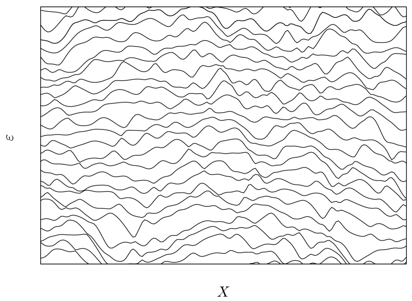
Figure 1: Parametric dependence of the energy levels of a tight-binding Anderson Hamiltonian on a $20\times 20$ lattice as a function of the strength $X$ of a fixed global perturbation (arbitrary units). To place the system in the unitary symmetry class, we have imposed an external random vector potential in addition to the random scalar potential.

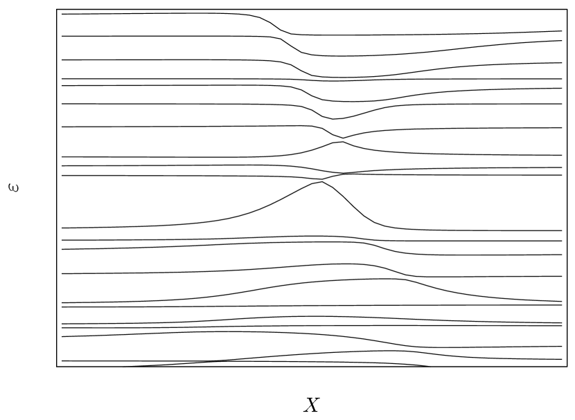
Figure 2: Parametric dependence of the energy levels of a time-reversal-invariant tight-binding Anderson Hamiltonian on a $20\times 20$ lattice as a function of the overall strength $X$ of an external perturbation localized on two fixed sites (arbitrary units).

Given these qualitative differences, the universality of the corresponding parametric correlations cannot be automatically deduced from the analysis of Refs. simons_altshuler ; altshuler_simons . In this paper, we utilize the NL$\sigma$M approach to prove the universality of the results in SMS ; SS1 ; SS2 and to establish their limits of applicability and, crucially, their parametrization in terms of non-universal ($H_{0}$-dependent) quantities. We also establish a precise criterion for the crossover between the localized SMS ; SS2 and extended simons_altshuler ; altshuler_simons regimes. The NL$\sigma$M also affords an extension of some of the previously obtained results to the orthogonal ensemble, although a complete counterpart of the results of Refs. SMS ; SS1 ; SS2 in the orthogonal case is unattainable at present.

II Parametric spectral correlation functions

The parametric analog of Eq. (1) – and the basic object to which we devote most of the attention in this paper – is the cross-correlation function

$$R_{11}(\Omega,V)=\bar{\Delta}^{2}\langle\nu(\varepsilon+\Omega/2;0)\;\nu(\varepsilon-\Omega/2;V)\rangle\;,$$ (6)

where $\nu(\varepsilon;V)=\operatorname{tr}\delta(\varepsilon-H-V)$. The notation is dictated by the fact that $R_{11}$ is the special case of the multi-point correlation function $R_{nm}$ involving $n$ densities $\nu(\varepsilon_{i};0)$ and $m$ ‘shifted’ densities $\nu(\varepsilon_{j};V)$. (Within this classification scheme, $R_{2}$ is more properly denoted as $R_{20}$.) Its universal form (in the case of random Hamiltonians of unitary symmetry) is given, as established in Refs. simons_altshuler ; altshuler_simons for global $V$, by the following expression:

$$R_{11}(s,V)-1\\ =\displaystyle\frac{1}{2}\mathrm{Re}\int_{1}^{\infty}d\lambda_{1}\int_{-1}^{1}d\lambda\;e^{i\pi s_{+}(\lambda_{1}-\lambda)-\sigma(\lambda,\lambda_{1};x_{0})}\;,$$ (7)

where

$$\sigma(\lambda,\lambda_{1};x_{0})\equiv\sigma_{\text{gl}}(\lambda,\lambda_{1};x_{0})=\pi^{2}x_{0}^{2}(\lambda_{1}^{2}-\lambda^{2})/2\;,$$ (8)

and $x_{0}$ is given by Eq. (5). Note that the resolvent of the diffusion operator $\Pi({\mathbf{r}},{\mathbf{r}}^{\prime})$ is a long-range object, so that the extended character of $V$ is essential in the structure of Eq. (5). Note also that $\Pi$ is smooth on the scale of the mean free path $\ell$, suppressing the contribution of the fast components of $V$ to (5).

The basic conclusion of the analysis presented in this paper is that in the case of a local perturbation (or a perturbation which has both global and local components) the overall structure of Eq. (7) is preserved, while the function $\sigma(\lambda,\lambda_{1};x_{0})$ is generalized to

$$\sigma(\lambda,\lambda_{1};x_{0},{\mathbf{x}})=\sigma_{\text{gl}}(\lambda,\lambda_{1};x_{0})+\sigma_{\text{loc}}(\lambda,\lambda_{1};{\mathbf{x}})$$

$$\sigma_{\text{loc}}(\lambda,\lambda_{1};{\mathbf{x}})=\sum_{a=1}^{r}\left[\ln\left(1+ix_{a}\lambda_{1}\right)-\ln\left(1+ix_{a}\lambda\right)\right]\;,$$ (9)

where the ‘local’ part $\sigma_{\text{loc}}$ of $\sigma$ depends on a vector of parameters ${\mathbf{x}}$. The vector ${\mathbf{x}}$ has a finite number $r$ of components, reflecting the finite extent of the local component of $V$. We also find an additional contribution to $x_{0}^{2}$, which properly accounts for the fast spatial oscillations in the extended parts of $V$,

$$\delta x_{0}^{2}=4\bar{\nu}^{2}\int d{\mathbf{r}}d{\mathbf{r}}^{\prime}V({\mathbf{r}})f_{d}^{2}({\mathbf{r}}-{\mathbf{r}}^{\prime})V({\mathbf{r}}^{\prime})X^{2}\;,$$ (10)

where $\bar{\nu}=1/\bar{\Delta}L^{d}$ is the average local DoS in a $d$-dimensional sample. The Friedel function $f_{d}({\mathbf{r}})$ represents the averaged Green function of a disordered system, and is given by

$$f_{d}({\mathbf{r}})=J_{d/2-1}(p_{F}r)e^{-r/2\ell}\;,$$ (11)

where $J_{\eta}$ is the Bessel function of $\eta$-th order.

In what sense is Eq. (9) universal, depending, as it does, on a whole list of parameters? To answer this question one needs to clarify whether analogs of Eq. (4) can be defined, i.e., whether these correlation functions are determined by an (at most finite) set of phenomenological parameters rather than the thermodynamically large number of variables in the pair of matrices $H_{0}$ and $V$.

As will be explained shortly, $x_{a}$ are nonlinear functions of $XV$. In other words, the transformation analogous to (4), if it exists at all, is non-linear – in contrast to the simple rescaling required in the global case. The nonlinearity means that, unlike the case of a global perturbation, the overall magnitude of the perturbation $X$ is no longer a ‘natural’ variable with respect to which level velocity should be defined. It is not even a priori clear that such a ‘natural’ variable exists.

There is, however, an extra requirement that can be imposed to make the parametrization unique. To help motivate it, let us note that, in the global case, $\sigma$ as a function of $x_{0}$ is essentially a Taylor expansion where terms of the order higher than $2$ vanish in the thermodynamic limit. As a result, correlation functions between $H+X_{1}V$ and $H+X_{2}V$ for arbitrary $X_{1}$ and $X_{2}$ are functions of the (properly rescaled) difference $X_{2}-X_{1}$. This translationally invariant parametrization is a direct consequence – in fact, the primary manifestation – of the principle of stationarity discussed in the Introduction. On general grounds, such stationarity should characterize parametric correlations induced by local perturbations as well. Thus, there must exist a ‘natural’ set of variables ${\mathbf{y}}({\mathbf{x}})$ possessing the following property: there is at least one curve connecting $H_{0}$ and $H_{0}+V$ such that the correlations between any two Hamiltonians on this curve corresponding to two different values $X_{1}$ and $X_{2}$ are functions of the differences ${\mathbf{y}}({\mathbf{x}}_{2})-{\mathbf{y}}({\mathbf{x}}_{1})$. The distribution of level velocities along this curve is independent of the position on the curve. In fact, for $r>1$, such curves are not unique, but rather span an $r$-dimensional manifold.

It is worth emphasizing that the existence of such parametrization is a non-trivial property even for a single parameter ($r=1$). For example, let us consider an arbitrary function $f(X_{1},X_{2})$. The existence of a ‘natural’ set of variables is equivalent to the requirement that for any $X_{1}$ and $X_{2}$ the function $f(X_{1},X_{2})$ can be represented as $g(h(X_{2})-h(X_{1}))$ for some functions $g$ and $h$. Such a representation clearly exists only for a very restricted subset of all possible $f$. As follows from the analysis below, the ‘natural’ parametrization does indeed exist, and it is effected by the substitution

$$y_{a}=\arctan x_{a}\;.$$ (12)

As will be shown in Section III, $x_{a}$ are the eigenvalues of the reactance matrix

$$\mathcal{R}\equiv i(\mathcal{S}-\openone)(\mathcal{S}+\openone)^{-1}\;,$$ (13)

where the scattering matrix $\mathcal{S}$ describes scattering off $V$ with free propagation controlled by the Green function of $H=H_{0}+H_{\text{dis}}$ averaged over $H_{\text{dis}}$. The emergence of the reactance matrix as a key object governing parametric correlations is rather natural within the formal framework presented in the subsequent Section. However, it is less obvious on an intuitive level, especially so since the reactance matrix is used much less frequently in the scattering theory proper than its ‘cousin’ the $T$-matrix (a very detailed exposition of the subject can be found, however, in newton ). Nevertheless, it can be qualitatively understood based precisely on the fact that reactance matrix is the Hermitian analog of the $T$-matrix. Indeed, the latter is conventionally defined by the equation $V|\chi_{\text{out}}\rangle=\mathcal{T}|\chi_{0}\rangle$, where $|\chi_{0}\rangle$ is the incident plane wave, and $|\chi_{\text{out}}\rangle$ is the scattered wave, normalized to unit flux. Similarly, $\mathcal{R}$ satisfies an equation of identical structure, $V|\varphi_{V}\rangle=\mathcal{R}|\varphi_{0}\rangle$, where $|\varphi_{V}\rangle$ and $|\varphi_{0}\rangle$ are now the conventionally normalized respectively, perturbed, and unperturbed, states in a closed system. Since we consider the parametric correlations of the real eigenvalues of Hermitian Hamiltonians in closed systems, reactance matrix is indeed quite a natural object to appear.

The eigenvalues of $\mathcal{R}$ are expressed as tangents of the corresponding eigenphases (scattering phase shifts) of $\mathcal{S}$. The parameters $y_{a}$ introduced in Eq. (12) thus have an intuitive physical interpretation as the corresponding phase shifts. The expression of $x_{a}$ (or $y_{a}$) in terms of the reactance matrix should be regarded as the analog of the microscopic definition of $x_{0}$ given by Eq. (5). Moreover, the fact that the ’natural’ parameters are the eigenvalues of the corresponding reactance matrix allows for a more direct definition of the special set of curves in the space of Hamiltonians which were discussed above. These curves can now be represented as sequences of Hamiltonians which map onto commuting sequences of reactance matrices.

It is possible to complete the analogy with the case of extended perturbations by establishing a counterpart of Eq. (4). The distribution $P(u)$ of level velocities $u=\partial\varepsilon_{i}/\partial|{\mathbf{y}}|$ can be extracted from Eq. (9) with the help of the identity kravtsov_zirnbauer :

$$P(u)=\lim_{|{\mathbf{y}}|\to 0}|{\mathbf{y}}|R_{11}(\Omega/\bar{\Delta}=u|{\mathbf{y}}|,{\mathbf{y}})\;.$$ (14)

Making use of this identity, one obtains the following result

$$P(u)=\mathrm{Re}\int_{0}^{\infty}d\zeta\;e^{i\pi u_{+}\zeta}\;e^{-\sum_{a}^{r}\ln(1+i\zeta\kappa_{a})}\;,$$ (15)

where $\kappa_{a}=y_{a}/|{\mathbf{y}}|$. Thus, the cumulants $C_{m}$ of the level velocity are given by

$$C_{m}=\displaystyle\frac{(m-1)!}{\pi^{m}}\sum_{a=1}^{r}\kappa_{a}^{m}\;.$$ (16)

By choosing $|{\mathbf{y}}|$ as the variable, we have already effectively performed a rescaling analogous to (4) (up to a factor of $\pi$), with $C_{2}\equiv C(0)$. Any set of additional $r-1$ cumulants is sufficient to invert Eq. (16), thus providing the remaining (non-linear) variable transformations between phenomenological constants $C_{m}$ and universal parameters $y_{a}$. Equation (16) establishes the universality of Eq. (9).

Although we have kept the discussion above rather general, the most interesting application from the practical point view is when $V$ is diagonal in the coordinate representation, and $H_{0}$ and $H_{\text{dis}}$ together describe weakly disordered metals. The latter are characterized by the hierarchy of scales $L\gg\ell\gg\lambda_{F}$. In this case it is convenient to distinguish two subtypes of local perturbations $V$. In the first subtype, the spatial extent $l_{V}$ of $V$ is smaller than $\ell$. For such perturbing potentials, Eq. (9) can be more compactly rewritten as

$$\sigma_{\text{loc}}(\lambda,\lambda_{1};{\mathbf{x}})=\operatorname{tr}\left(1+i\mathcal{R}\lambda_{1}\right)\left(1+i\mathcal{R}\lambda\right)^{-1}\;,$$ (17)

where $\mathcal{R}$ is the reactance matrix projected onto the Fermi surface, and $\operatorname{tr}$ denotes the trace in the space of the scattering channels. The full reactance matrix is defined by the equation

$$\mathfrak{R}=(1-V\mathrm{Re}\langle G^{\text{\sc{r}}}\rangle)^{-1}V\;,$$

where the retarded average Green function is defined as $\langle G^{\text{\sc{r}}}\rangle\equiv\langle(\varepsilon_{F}-H_{0}-H_{\text{dis}}+i0)^{-1}\rangle$, so that $\mathfrak{R}$ is formally distinct from the average reactance matrix $\langle(1-V\mathrm{Re}G^{\text{\sc{r}}})^{-1}V\rangle$; nevertheless the difference between $\mathfrak{R}$ and the average reactance matrix enters only in the subleading order in $\lambda_{F}/\ell$, and can be ignored. Transforming to the momentum representation it is convenient to split off the angular variables in $\mathfrak{R}$ as $\mathfrak{R}({\mathbf{p}},{\mathbf{p}}^{\prime})=\mathfrak{R}(\xi,\hat{{\mathbf{n}}};\xi^{\prime},\hat{{\mathbf{n}}}^{\prime})$, where $\xi={\mathbf{p}}^{2}/2m-\varepsilon_{F}$. The projected reactance matrix $\mathcal{R}$ is defined as $\mathcal{R}_{\hat{{\mathbf{n}}},\hat{{\mathbf{n}}}^{\prime}}\equiv\pi\bar{\nu}\mathfrak{R}(0,\hat{\mathbf{n}};0,\hat{\mathbf{n}}^{\prime})$.

In the opposite limit $L\gg l_{V}\gg\ell$, Eq. (17) retains its structure provided $\mathcal{R}$ is replaced with

$$\mathcal{R}_{P}=P^{1/2}(\xi)\mathfrak{R}(\xi,\hat{{\mathbf{n}}};\xi^{\prime},\hat{{\mathbf{n}}}^{\prime})P^{1/2}(\xi^{\prime})\;,$$

where

$$P(\xi)=\displaystyle\frac{(1/2\pi\tau)}{\xi^{2}+(1/2\tau)^{2}}\;,$$

$\tau=\ell/v_{F}$ is the mean free time, and the trace operation $\operatorname{tr}$ is redefined to include the $\xi$ degrees of freedom. In other words, the projection onto the Fermi surface is smeared over a strip of width $1/2\tau$ around it, reflecting the fact that the average Green function exponentially decays over distances larger than $\ell$ so that a scatterer of size larger than $\ell$ is effectively split into independent chunks of size $\ell$. Since the algebraic structure of the parametric correlation functions is identical in both cases $l_{V}<\ell$ and $l_{V}>\ell$, below we will often omit the subscript $P$.

In summary, the two ways of defining ${\mathbf{y}}$ either in terms of the solutions of Eq. (16) or as the eigenphases of the reactance matrix stand in direct correspondence with the definition of $x_{0}$ either phenomenologically (4) or microscopically (5). While very convenient for theoretical analysis, the definition in terms of the eigenphases is of little practical utility since measuring $\mathcal{R}$ is hardly feasible. On the other hand, cumulants of the level velocity distribution are readily accessible in appropriately designed experiments.

The universality of the parametric correlation functions is explicitly demonstrated through the existence of their translationally invariant parametrization in terms of the scattering phase shifts. In this context, the standard universal Wigner-Dyson statistics of energy levels (spectral points) could be viewed as the boundary condition to the universal statistics of spectral lines as functions of coordinates in the space of Hamiltonians.

II.1 Orthogonal ensemble

All of the preceding discussion can be applied verbatim to the case of orthogonal symmetry provided Eqs. (7) and (17) are replaced with

$$R_{11}^{(o)}(s,V)=1+\mathrm{Re}\int_{1}^{\infty}d\lambda_{1}d\lambda_{2}\int_{-1}^{1}d\lambda\;J(\lambda,\lambda_{1},\lambda_{2})e^{i\pi s_{+}(\lambda_{1}\lambda_{2}-\lambda)-\sigma^{(o)}(\lambda,\lambda_{1},\lambda_{2};x_{0},\mathbf{x})}\;,$$ (18)

where

$$J(\lambda,\lambda_{1},\lambda_{2})=\displaystyle\frac{(\lambda_{1}\lambda_{2}-\lambda)^{2}(1-\lambda^{2})}{(\lambda_{1}^{2}+\lambda_{2}^{2}+\lambda^{2}-2\lambda\lambda_{1}\lambda_{2}-1)^{2}}$$

and the global and local parts of $\sigma^{(o)}$ are given by, respectively,

$$\sigma_{\text{gl}}^{(o)}(\lambda,\lambda_{1},\lambda_{2};x_{0})=\displaystyle\frac{\pi^{2}x_{0}^{2}}{2}\left(1+2\lambda_{1}^{2}\lambda_{2}^{2}-\lambda^{2}-\lambda_{1}^{2}-\lambda_{2}^{2}\right)$$

and

$$\sigma_{\text{loc}}^{(o)}(\lambda,\lambda_{1},\lambda_{2};\mathbf{x})\\ =\displaystyle\frac{1}{2}\operatorname{tr}\ln\displaystyle\frac{\openone+2i\mathcal{R}\lambda_{1}\lambda_{2}-\mathcal{R}^{2}(\lambda_{1}^{2}+\lambda_{2}^{2}-1)}{(\openone+i\mathcal{R}\lambda)^{2}}\;.$$ (19)

As before, $\mathcal{R}$ has to be replaced with $\mathcal{R}_{P}$ with the corresponding redefinition of $\operatorname{tr}$ if $l_{V}\gg\ell$.

A similar set of expressions can also be written in the symplectic ($\beta=4$) case.

II.2 Level velocity distribution and Berry’s conjecture

Applying Eq. (14) to Eq. (18), we find that Eq. (15) is a special case of a more general expression:

$$P(u)=\displaystyle\frac{\beta}{2}\mathrm{Re}\int_{0}^{\infty}d\zeta\;e^{i\pi\beta u_{+}\zeta/2}\;e^{-(\beta/2)\sum_{a}^{r}\ln(1+i\zeta\kappa_{a})}\;.$$ (20)

It is interesting to note that the distribution of level velocities can be obtained using a completely different approach. As can be easily seen from the expansion of an arbitrary eigenvalue $\varepsilon_{i}$ of $H+XV$ to linear order in $X$,

$$\varepsilon_{i}(X)\simeq\varepsilon_{i}+XV_{ii}+O(X^{2})$$

$$V_{ii}=\int d{\mathbf{r}}\;|\psi_{i}({\mathbf{r}})|^{2}V({\mathbf{r}})\;,$$

the level velocity coincides with the expectation value of $V$ in the $i$-th eigenstate of $H$. Restricting our attention for simplicity to the case $l_{V}\ll\ell$, we can employ Berry’s conjecture about the distribution of wave function values in chaotic systems berry ; gornyi_mirlin :

$$\mathcal{P}[\psi]=\displaystyle\frac{1}{(\det\hat{f}^{-1})^{\beta/2}}e^{-(\beta/2)\int d{\mathbf{r}}d{\mathbf{r}}^{\prime}\psi^{\dagger}({\mathbf{r}})[\hat{f}^{-1}]_{{\mathbf{r}}{\mathbf{r}}^{\prime}}\psi({\mathbf{r}}^{\prime})}\;,$$

where in $d$ spatial dimensions the matrix elements of the integral operator $\hat{f}$ are given by the Friedel function (11), which in the limit $l_{V}\ll\ell$ can be approximated as $f_{d}({\mathbf{r}}-{\mathbf{r}}^{\prime})\equiv\int d{\mathbf{n}}\;e^{ip_{F}{\mathbf{n}}\cdot({\mathbf{r}}-{\mathbf{r}}^{\prime})}=J_{d/2-1}(p_{F}r)$. In this expression the integration is performed over all directions of the unit vector ${\mathbf{n}}$ and $r=|{\mathbf{r}}-{\mathbf{r}}^{\prime}|$. The fields $\psi$ are complex in the unitary case, and real for $\beta=1$. While originally conjectured for chaotic systems berry , this expression was recently proved gornyi_mirlin to hold locally in diffusive systems of unitary symmetry. We thus immediately find

$$P(u)=\bar{\Delta}\sum_{i}\langle\delta(u-V_{ii}/\bar{\Delta})\delta(\varepsilon-\varepsilon_{i})\rangle\\ =\int_{-\infty}^{+\infty}\displaystyle\frac{d\zeta}{2\pi}\int D\psi_{i}\mathcal{P}[\psi_{i}]\;e^{iu\zeta-i\zeta\int d{\mathbf{r}}\;|\psi_{i}({\mathbf{r}})|^{2}V({\mathbf{r}})/\bar{\Delta}}\\ =\int_{-\infty}^{\infty}\displaystyle\frac{d\zeta}{2\pi}\;e^{i\zeta u}\displaystyle\frac{1}{[\det(\openone+2i\zeta\hat{f}V/\beta\bar{\Delta})]^{\beta/2}}\;.$$ (21)

The last expression can be shown to coincide with Eq. (20), thus indirectly confirming the validity of Berry’s conjecture in diffusive systems of orthogonal symmetry. Indeed, $y_{a}/|{\mathbf{y}}|$ coincide with the eigenvalues of the Fermi surface projection of $d\mathcal{R}/dX|_{X\to 0}\equiv V$. The corresponding projected matrix elements are $\int d{\mathbf{r}}\;e^{ip_{F}({\mathbf{n}}-{\mathbf{n}}^{\prime})\cdot{\mathbf{r}}}V({\mathbf{r}})$. Using the integral decomposition of $f_{d}({\mathbf{r}}-{\mathbf{r}}^{\prime})$ and the cyclic invariance of the determinant, the equivalence of Eqs. (20) and (21) is immediately established. This analysis can also be in an obvious way extended to the case $L\gg l_{V}\gg\ell$.

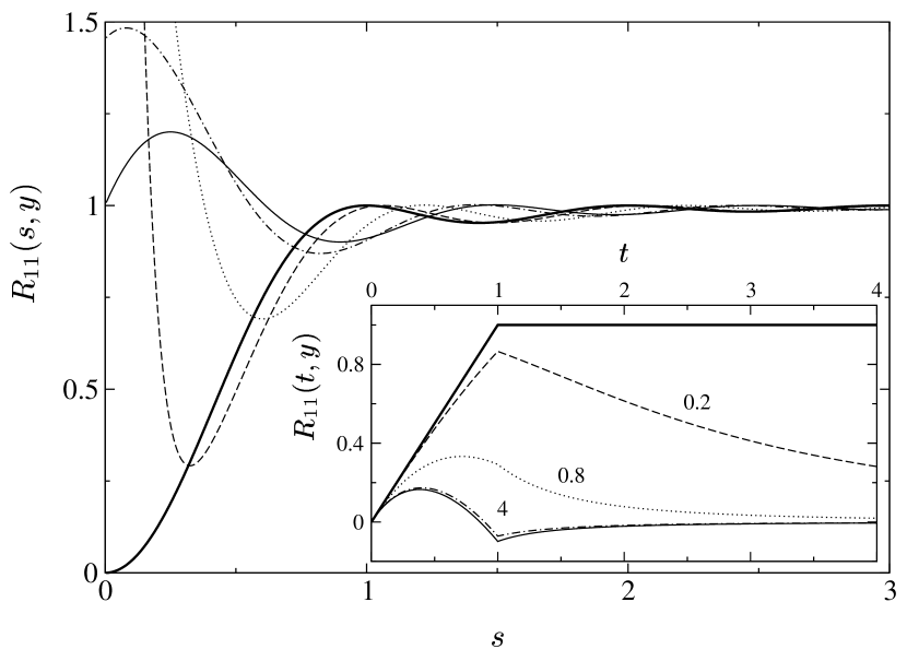
Figure 3: DoS-DoS correlation function for the rank $r=1$ problem, $R_{11}(s,y)$, for different strengths $\tan y$ of the perturbing potential: $\tan y=0.2$ (dashed line), $\tan y=0.8$ (dotted line), $\tan y=4$ (dot-dashed line), $\tan y\to\infty$ (solid line), while the bold line corresponds to the GUE Wigner-Dyson result, $y=0$. The corresponding Fourier transforms are shown in the inset.

II.3 Examples

Before turning to derivation of the above results, it is instructive to analyze several special cases. For example, if $V$ models a collection of several impurities, it can be approximated as

$$V({\mathbf{r}})=\displaystyle\frac{1}{\bar{\nu}}\sum_{k=1}^{r}v_{k}\delta({\mathbf{r}}-{\mathbf{r}}_{k})\;.$$ (22)

Crudely speaking, a bistable impurity would have $r=2$ and $v_{1}=-v_{2}$, while a local defect created, e.g., by irradiation would correspond to $r=1$.

Throughout this subsection we largely restrict the discussion to the unitary ensemble. The corresponding results for $\beta=1$ can be straightforwardly obtained in terms of the corresponding $\lambda$ integrals starting from Eq. (19).

Despite the fact that $\mathcal{R}$ (or $\mathcal{R}_{P}$) is a continuous integral operator, the structure of Eq. (22) ensures that it possesses exactly $r$ non-zero eigenvalues. Using the cyclic invariance of the trace, the latter are easily seen to coincide with the eigenvalues of the asymmetric matrix $M_{kk^{\prime\prime}}=\sum_{k^{\prime}=1}^{r}\mathcal{R}({\mathbf{r}}_{k},{\mathbf{r}}_{k^{\prime}})f_{d}({\mathbf{r}}_{k^{\prime}}-{\mathbf{r}}_{k^{\prime\prime}})$, where, for arbitrary $l_{V}\ll L$, the Friedel function $f_{d}({\mathbf{r}})$ is given by Eq. (11).

In the simplest $r=1$ case, $M_{kk^{\prime}}$ is a number, $\tan y=v/(1-\alpha v)$, where for brevity we denote $\alpha=\mathrm{Re}\langle G^{\text{\sc{r}}}({\mathbf{r}}=0)\rangle/\bar{\nu}$, and the correlation function in the unitary ensemble can be explicitly written in the form (assuming $y>0$)

$$R_{11}(s,y)-1=-\left\{\displaystyle\frac{\partial}{\partial s}\left[e^{-\pi s\cot y}k(s)\right]\right\}\\ \left[\theta(s)-\int_{-\infty}^{s}ds^{\prime}e^{\pi s^{\prime}\cot y}k(s^{\prime})\right]\;,$$ (23)

where the function $k(s)$ has been defined in (3), therefore reproducing the result obtained previously aleiner_matveev using RMT methods. The function $R_{11}$ for $r=1$ is plotted in Fig. 3 for several different values of $y$ together with its Fourier transform. One can clearly see the gradual broadening of the central peak inherited from the $\delta$-function term in Eq. (2). At small values of $y$ the dominant contribution to the broadened peak comes from the correlations between a level and its parametric ‘descendant’. It is also worth noting that the parametric correlation function inherits from its non-parametric limit the sharp oscillatory behavior which is reflected in the singularity (cusp) in its Fourier transform

$$R_{11}(t,y)=\int_{-\infty}^{\infty}ds\;e^{-2\pi ist}R_{11}(s,y)\\ =\delta(t)+\min(t,1)+\displaystyle\frac{t}{2}\ln\left[\displaystyle\frac{1+\tan^{2}yg^{2}(t)}{1+\tan^{2}y(1+2t)^{2}}\right]\;,$$

where $g(t)=2t-2\min(t,1)+1$. Although not directly obvious from Eq. (23), the perturbed levels in the $r=1$ case possess the property (for $y>0$) $\varepsilon_{i}<\varepsilon_{i}(y)<\varepsilon_{i+1}$ aleiner_matveev . This feature is clearly illustrated in Fig. 4.

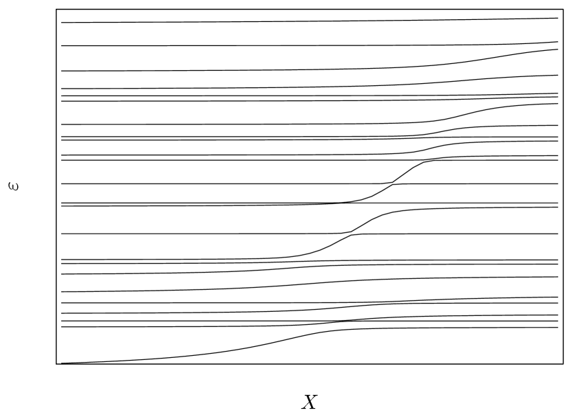
Figure 4: Dependence of the energy levels on the overall strength $X$ of an external local (i.e., localized on a single site) perturbation $V$ for a time-reversal invariant tight-binding $20\times 20$ lattice model (arbitrary units). Level anti-crossing and the property $\varepsilon_{i}<\varepsilon_{i}(X)<\varepsilon_{i+1}$ aleiner_matveev are clearly shown.

In the $r=2$ case we restrict our attention to modeling a bistable impurity, thus setting $v_{1}=-v_{2}=v>0$, and $r_{12}\ll\ell$. Denoting as before $\alpha=\mathrm{Re}\langle G^{\text{\sc{r}}}({\mathbf{r}}=0)\rangle/\bar{\nu}$, and also $\gamma=\mathrm{Re}\langle G^{\text{\sc{r}}}(r_{21})\rangle/\bar{\nu}$, $r_{kk^{\prime}}=|{\mathbf{r}}_{k}-{\mathbf{r}}_{k^{\prime}}|$, and $f_{kk^{\prime}}=f_{d}(r_{kk^{\prime}})$, we find

$$\tan y_{1,2}=\displaystyle\frac{v^{2}(\alpha-\gamma f_{12})\pm v\sqrt{1-f_{12}^{2}+v^{2}(\alpha f_{12}-\gamma)^{2}}}{1-v^{2}(\gamma^{2}-\alpha^{2})}\;.$$

In the limit $r_{12}\to 0$ both eigenvalues, as expected, vanish. We omit somewhat lengthy explicit expressions for $R_{11}$ and its Fourier transform, presenting instead in Fig. 5 the corresponding graphs at several different values of $y$. The limit $r_{12}\to 0$ can also be used to extract the distribution of level velocities due to a moving impurity. Expanding $1-f_{12}\approx(1/2d)p_{F}^{2}r^{2}$ we find (setting for simplicity $\alpha=\gamma=0$) that the distribution of $u=\partial\varepsilon_{i}/\partial(p_{F}r)$ is Poissonian:

$$P(u)=\displaystyle\frac{\sqrt{d}}{2v}e^{-|u|\sqrt{d}/v}\;.$$ (24)

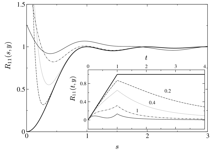
Figure 5: DoS-DoS correlation function for the rank $r=2$ problem, $R_{11}(s,y)$, for different values of $\tan y=\tan y_{1}=-\tan y_{2}$. The bold line corresponds to the GUE Wigner-Dyson result, $\tan y=0$, while $\tan y=0.2$ (dashed line), $\tan y=0.4$ (dotted line), $\tan y=1$ (dot-dashed line), $\tan y\to\infty$ (solid line). The corresponding Fourier transforms are shown inset.

This result can be generalized to study the response of the energy levels to a shift in the position of an extended defect. An experimentally relevant application is the lateral motion of an STM tip over a disordered two-dimensional electron gas. Another example is a metallic scatterer inside a microwave ‘billiard’ such as those studied in Ref. sridhar .

Approximating the potential $U$ of an STM tip as a flat disk of radius $\rho$, $U({\mathbf{r}})=U_{0}\theta(\rho^{2}-{\mathbf{r}}^{2})$, and denoting the displacement of the center of the disk as $\lambda$, the difference between the potentials produced at two adjacent positions of the disk is given, to the first order in $\lambda$, by $V({\mathbf{r}})\equiv V(r,\phi)=2U_{0}\lambda\rho\delta({\mathbf{r}}^{2}-\rho^{2})\cos\phi$, where the direction of the displacement corresponds to $\phi=0$. Therefore, neglecting the $O(U_{0})$ corrections to $f_{d}({\mathbf{r}})=J_{0}(p_{F}r)$, one finds that the operator $\hat{f}V/\bar{\Delta}$ appearing in the expression for the velocity distribution (21) reduces to a continuous integral operator defined on a circle $0\leq\phi<2\pi$:

$$\kappa(\phi,\phi^{\prime})=\displaystyle\frac{1}{2\pi}J_{0}(2p_{F}\rho\sin((\phi-\phi^{\prime})/2))\cos\phi^{\prime}\;.$$

Since the corresponding eigenvalues $\kappa_{a}$ are symmetric with respect to zero, the distribution of level velocities can be written as

$$P_{\text{\sc{stm}}}(u/\bar{u})=\int_{-\infty}^{\infty}\displaystyle\frac{d\zeta}{2\pi}e^{i\zeta(u/\bar{u})-(\beta/2)\sum_{\kappa_{a}>0}\ln[1+(2\kappa_{a}\zeta/\beta\bar{u})^{2}]}\;,$$

where the average velocity $\bar{u}$ is given by

$$\bar{u}^{2}\equiv\langle u^{2}\rangle=\displaystyle\frac{2}{\beta}\sum_{a}\kappa_{a}^{2}\\ =\displaystyle\frac{1}{\beta\pi}\int_{0}^{\pi}d\theta J_{0}^{2}(2p_{F}\rho\sin\theta)\cos(2\theta)\;.$$

In the unitary case, $\beta=2$, the distribution function (Fig. 6) shows a crossover from Poisson to Gaussian behavior as $p_{F}\rho$ increases, while in the orthogonal case (Fig. 7) the crossover is between the limiting behavior described by the modified Bessel function $(1/\pi)K_{0}(|u|)$ barth and the Gaussian limit. These crossovers explicitly illustrate the distinction between local and global perturbations, and show that the global regime is achieved when the central limit theorem comes into force due to a large number of distinct eigenvalues $\kappa_{a}$. Such a crossover has been observed in experiments on microwave resonators barth where the appropriate ensemble is orthogonal.

A new feature appearing in this example is that a local potential is described by a formally infinite number of the eigenvalues $\kappa_{a}$ of an integral operator. However, the finite extent of $V$ guarantees that all but a finite number of these eigenvalues are vanishingly small, so that, depending on the required degree of accuracy, there can always be defined an appropriate finite value of $r$.

III Field Theory of Parametric Correlations

We turn now to the derivation of the results presented in the preceding Section. To explore the influence of a local potential perturbation on the ensemble average properties of the weakly disordered system, we will employ a conventional approach based on the supersymmetric field theoretic formulation. Since this approach has been reviewed extensively in the literature efetov , we will keep our discussion here concise, paying particular attention only to the idiosyncrasies of the present scheme.

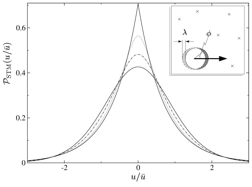
Figure 6: Graph of $P_{\text{\sc{stm}}}(u/\bar{u})$ in the unitary ensemble obtained for $p_{F}\rho=1.5$ and $4.0$ together with the limiting cases of Poisson ($p_{F}\rho\rightarrow 0$) and Gaussian ($p_{F}\rho\rightarrow\infty$) distributions. The inset shows the perturbation $V({\mathbf{r}})$ arising from the displacement of the disk-shaped potential.

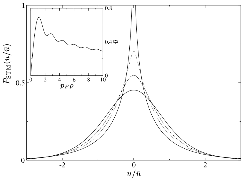
Figure 7: Graph of $P_{\text{\sc{stm}}}(u/\bar{u})$ in the orthogonal ensemble obtained for $p_{F}\rho=1.8$ and $p_{F}\rho=5$ together with the limiting cases of $p_{F}\rho\rightarrow 0$ and $p_{F}\rho\rightarrow\infty$. The inset shows $\bar{u}=\langle u^{2}\rangle^{1/2}$ as a function of $p_{F}\rho$.

Focusing on the weakly disordered system, our starting point is the set of single-particle Hamiltonians

$$H_{i}=\hat{\xi}_{\hat{{\mathbf{p}}}-e{\mathbf{A}}}+U({\mathbf{r}})+V_{i}({\mathbf{r}})\;,$$

where $\hat{\xi}_{\hat{{\mathbf{p}}}-e{\mathbf{A}}}=(\hat{{\mathbf{p}}}-e{\mathbf{A}})^{2}/2m-\varepsilon_{F}$ is the kinetic energy operator a free-particle system subject to an external vector potential ${\mathbf{A}}$. The impurity potential $U({\mathbf{r}})$ is drawn at random from a Gaussian $\delta$-correlated distribution with zero mean, and variance

$$\langle U({\mathbf{r}})U({\mathbf{r}}^{\prime})\rangle=\displaystyle\frac{1}{2\pi\bar{\nu}\tau}\delta({\mathbf{r}}-{\mathbf{r}}^{\prime})\;,$$ (25)

where $\tau$ is the associated elastic mean free time, $\tau=\ell/v_{F}$. In the following, we will limit our considerations to the diffusive regime, where the sample size $L$ is greatly in excess of the mean free path $\ell$ and where the wavefunction is extended over the volume of the system. Moreover the energy scales are arranged in the hierarchy

$$\varepsilon_{F}\gg\displaystyle\frac{1}{\tau}\gg E_{c}\gg\bar{\Delta}\;,$$

with $E_{c}=D/L^{2}$ and $D=v_{F}^{2}\tau/d$. In addition to the random potential $U({\mathbf{r}})$, the diffusive system is subject to a further (potentially short-ranged) arbitrary external parametric perturbation which can take $n$ values $V_{i}({\mathbf{r}})$.

Our goal initially is to construct a formalism which allows, at least in principle (see below), to compute multi-point correlation functions of the DoS,

$$R({\boldsymbol{\varepsilon}};{\mathbf{V}})=\langle\prod_{i=1}^{p}\nu(\varepsilon_{i};V_{i})\rangle\;,$$ (26)

where ${\boldsymbol{\varepsilon}}$ and ${\mathbf{V}}$ denote $p$-dimensional vectors with components $\varepsilon_{i}$ and $V_{i}$, respectively, and $\nu(\varepsilon_{i};V_{i})$ is the value of the density of states at energy $\varepsilon_{i}$ of the Hamiltonian $\hat{\xi}_{\hat{{\mathbf{p}}}}+U+V_{i}$. For generality, let us assume that $p\geq n$, so that some of $V_{i}$ in  (26) are equal. The $p$ energies in ${\boldsymbol{\varepsilon}}$ (which are generically different) are correspondingly split into $n$ groups of size $p_{j}$, each group matching a given value $V_{j}$. Moreover, from now on, we assume that the Fermi energy $\varepsilon_{F}$, which is included in the free Hamiltonian $\hat{\xi}_{\hat{{\mathbf{p}}}}$, is subtracted from the energies $\varepsilon_{i}$.

According to the standard methods efetov ; altshuler_simons , the generating functional required to construct a field-theoretic representation of $R({\boldsymbol{\varepsilon}};{\mathbf{V}})$ in the case of unbroken time-reversal symmetry is written as a functional integral over an $8p$-dimensional supermultiplet of complex fields:

$$\mathcal{Z}[j]=\int D(\psi^{\dagger},\psi)\exp\left\{i\int d{\mathbf{r}}\left\{\bar{\Psi}\left[\widehat{\varepsilon}^{\;c}-\hat{\xi}_{\hat{{\mathbf{p}}}}-U({\mathbf{r}})-\widehat{V}({\mathbf{r}})\right]\Psi+\Psi^{\dagger}j+j^{\dagger}\Psi\right\}\right\}\;,$$ (27)

where, by choosing the fields $\psi$ to consist of $2p$ copies of both boson (b) and fermion (f) elements, the normalization of the generating function, $\mathcal{Z}[0]=1$ is enforced. The factor $2$ in $2p$ is explained by the need to generate both retarded (r) and advanced (a) Green functions, so that $\varepsilon_{i}^{c}=(\varepsilon_{i}\sigma_{0}^{\text{\sc{ra}}}+\sigma_{3}^{\text{\sc{ra}}}i0)\otimes\sigma_{0}^{\text{\sc{bf}}}\otimes\sigma_{0}^{\text{\sc{tr}}}$. The further doubling of the number of components of the superfields is dictated by the need to properly take into account the soft modes associated with the time-reversal invariance of the Hamiltonian (hence the notation tr for the corresponding subspace):

$$\Psi =\displaystyle\frac{1}{\sqrt{2}}\begin{pmatrix}\psi\\ \psi^{*}\end{pmatrix}_{\text{\sc{tr}}} \begin{split}\Psi^{\dagger}&=\left(C\Psi\right)^{\mathsf{T}}\\ \Psi&=C(\Psi^{\dagger})^{\mathsf{T}}\;,\end{split}$$

where $C=\sigma_{1}^{\text{\sc{tr}}}\otimes E_{11}^{\text{\sc{bf}}}+i\sigma_{2}^{\text{\sc{tr}}}E_{22}^{\text{\sc{bf}}}$, and the $E$-matrices are the projectors onto the corresponding parts of the superspace. To stay close to the conventional notation adopted in the literature, in the following we will denote $\sigma_{3}^{\text{\sc{ra}}}\equiv\Lambda$. The conjugate superfields are defined by $\bar{\psi}=\psi^{\dagger}L$, where $L=\Lambda\otimes E_{11}^{\text{\sc{bf}}}+\openone\otimes E_{22}^{\text{\sc{bf}}}$ (further details on notation can be found in efetov ). Finally, $\widehat{\varepsilon}^{\;c}=\operatorname{diag}(\varepsilon_{1}^{c},\dots,\varepsilon_{p}^{c})$, $\widehat{V}=\operatorname{diag}(V_{1},\dots,V_{p})$, and the absence of an explicit operator in any subspace always implies the corresponding identity operator.

The only exception to this structure is the case $p=2$, where it is sufficient to represent each of the two DoS factors by either a retarded or an advanced Green function, with the opposite choice for the remaining factor, thus reducing the number of required components of the superfields from $16$ to $8$.

An ensemble average of the generating functional $\mathcal{Z}[j]$ over realizations of the random impurity potential $U({\mathbf{r}})$ induces a quartic interaction of the fields $\Psi$, which can be decoupled by means of a Hubbard-Stratonovich transformation with the introduction of $8p\times 8p$-component supermatrix fields $\mathcal{Q}({\mathbf{r}})$. In the absence of symmetry breaking sources, the resulting action is invariant under pseudounitary transformations, $\mathcal{Q}\mapsto T\mathcal{Q}T^{-1}$, where $T$ satisfies $T^{\dagger}LT=L$, and thus belongs to the pseudounitary supergroup $\mathrm{U}(2p,2p|4p)$. Moreover, $\mathcal{Q}$ satisfies the time-reversal symmetry constraint $\mathcal{Q}=LC^{\mathsf{T}}\mathcal{Q}^{\mathsf{T}}CL$.

After performing the integration over the superfields $\Psi$, one obtains the ensemble-averaged generating functional

$$\langle\mathcal{Z}[0]\rangle=\int D\mathcal{Q}\;e^{-S[\mathcal{Q}]}\;,$$

where the action $S[\mathcal{Q}]$ is

$$S[\mathcal{Q}]=-\displaystyle\frac{\pi\bar{\nu}}{8\tau}\int d{\mathbf{r}}\;\operatorname{str}\mathcal{Q}^{2}+\frac{1}{2}\int d{\mathbf{r}}\;\operatorname{str}\langle{\mathbf{r}}|\ln\hat{\mathcal{G}}^{-1}|{\mathbf{r}}\rangle\;,$$ (28)

and

$$\mathcal{G}^{-1}[\mathcal{Q};\widehat{V}]=\widehat{\varepsilon}^{\;c}-\hat{\xi}_{\hat{{\mathbf{p}}}}-\widehat{V}({\mathbf{r}})+\displaystyle\frac{i}{2\tau}\mathcal{Q}({\mathbf{r}})$$

denotes the supermatrix Green function. The description of the structure of supermatrices and the definition of the supertrace (here, $\operatorname{str}=\operatorname{tr}_{\text{\sc{b}}}-\operatorname{tr}_{\text{\sc{f}}}$) operation can be found in efetov .

The action (28) possesses an almost degenerate saddle-point manifold. Varying the action with respect to $\mathcal{Q}$, one obtains the saddle-point equation

$$\mathcal{Q}({\mathbf{r}})=\displaystyle\frac{i}{\pi\bar{\nu}}\langle{\mathbf{r}}|\mathcal{G}[\mathcal{Q};\widehat{V}]|{\mathbf{r}}\rangle\;.$$ (29)

This equation can be interpreted as the self-consistent Born approximation for the self-energy of the supermatrix Green function. The ambiguity involved in choosing among the different disconnected solutions of this equation is resolved by taking into account the analytical properties of the average Green function: $\mathcal{Q}=\Lambda$. In the limit $\widehat{\varepsilon}\to 0$ and $\widehat{V}\to 0$, the saddle-point solution expands to fill the degenerate manifold generated by transformations $\mathcal{Q}=T\Lambda T^{-1}$, where $T\in\mathrm{U}(2p,2p|4p)$.

III.1 The Non-Linear $\sigma$ Model

In the standard scheme efetov leading to the NL$\sigma$M structure of the field theory, the fluctuations of $\mathcal{Q}$ in the direction perpendicular to the saddle-point manifold are massive due to the inequality $p_{F}\ell\gg 1$. Moreover, in the leading order in $1/p_{F}\ell$, these fluctuations are quadratic and independent of the transverse fluctuations. As a result, integration over the massive modes does not lead to any modifications of the saddle point action apart from an overall constant multiplying $\mathcal{Z}$; supersymmetry further ensures that the constant is equal to $1$. In the case of global parametric perturbations this scheme is preserved altshuler_simons ; simons_altshuler due to the fact that $V({\mathbf{r}})$ is locally small, as discussed above. However, it is not a priori obvious that the same is true in the case of local perturbations, since the latter are locally large. Therefore, care has to be exercised in the derivation of the parametric version of NL$\sigma$M to demonstrate that (i) local perturbations do not destroy locally the saddle-point structure (i.e. that the distinction between the massless transverse and massive longitudinal fluctuations is preserved), and (ii) that any possible cross-couplings between massive and soft modes mediated by $V$ do not modify the saddle-point action in the leading order in $1/p_{F}\ell$.

To undertake this program, we begin by separating the fluctuations around the saddle-point manifold into transverse modes $Q({\mathbf{r}})$, which are nearly massless and slowly varying on the scale of the mean free path $\ell$, and massive modes $\delta Q_{m}({\mathbf{r}})$, in such a way that $\mathcal{Q}({\mathbf{r}})=Q({\mathbf{r}})+\delta Q_{m}({\mathbf{r}})$. The latter include the longitudinal fluctuations $\delta Q_{l}$ as well as fast transverse fluctuations $\delta Q_{f}$. The need to account for fast transverse fluctuations arises from the fact that local perturbations vary rapidly on the scale of the wavelength $\lambda_{F}$, so that their coupling to fast transverse modes cannot a priori be ignored. In principle, a naïve inclusion of fast transverse fluctuations can lead to overcounting, as, e. g. a $2p_{F}$ Diffuson mode is a Cooperon, and vice versa. Nevertheless, below we will demonstrate that massive modes do not in fact generate any corrections to the slow mode action in the leading order in $1/p_{F}\ell$, and a detailed calculation of the subleading terms is not needed.

By definition, the longitudinal modes are orthogonal to the saddle-point manifold, therefore satisfying $[\delta Q_{l}({\mathbf{r}}),Q({\mathbf{r}})]=0$. In contrast, the slow transverse modes can be parametrized as $Q({\mathbf{r}})=T({\mathbf{r}})\Lambda T^{-1}({\mathbf{r}})$. The corresponding free supermatrix Green function, $\mathcal{G}_{0}[Q]=\mathcal{G}[\widehat{\varepsilon}^{\;c}=0,\delta Q_{m}=0;\widehat{V}=0]$, obeys the relation:

$$\mathcal{G}_{0}({\mathbf{r}},{\mathbf{r}}^{\prime})=\mathrm{Re}\langle G^{\text{\sc{r}}}({\mathbf{r}},{\mathbf{r}}^{\prime})\rangle\\ -i\pi\bar{\nu}f_{d}({\mathbf{r}}-{\mathbf{r}}^{\prime})Q\left(\displaystyle\frac{{\mathbf{r}}+{\mathbf{r}}^{\prime}}{2}\right)\;,$$

where the retarded Green function is defined as $G^{\text{\sc{r}}}=(-\hat{\xi}_{\hat{{\mathbf{p}}}}-U+i0)^{-1}$ and where $f_{d}({\mathbf{r}}-{\mathbf{r}}^{\prime})$ denotes the Friedel function (11).

Separating the $V$-dependent parts of the action, we represent it as

$$S[\mathcal{Q}]=S[Q]+\delta S[Q,\delta Q_{m}]\;,$$

where

$$S[Q]=-\displaystyle\frac{\pi\bar{\nu}}{8\tau}\int d{\mathbf{r}}\;\operatorname{str}Q^{2}+\displaystyle\frac{1}{2}\int d{\mathbf{r}}\;\operatorname{str}\langle{\mathbf{r}}|\ln\mathcal{G}^{-1}[Q]|{\mathbf{r}}\rangle\\ +\frac{1}{2}\int d{\mathbf{r}}\;\operatorname{str}\langle{\mathbf{r}}|\ln\left(\openone-\mathcal{G}[Q]\widehat{V}\right)|{\mathbf{r}}\rangle\;,$$ (30)

$\mathcal{G}[Q]\equiv\mathcal{G}[Q;\widehat{V}=0]$, and the expansion

$$\mathcal{G}[\mathcal{Q}]=\mathcal{G}[Q]-\displaystyle\frac{i}{2\tau}\mathcal{G}[Q]\delta Q_{m}\mathcal{G}[Q]\\ -\displaystyle\frac{1}{(2\tau)^{2}}\mathcal{G}[Q]\delta Q_{m}\mathcal{G}[Q]\delta Q_{m}\mathcal{G}[Q]$$

determines the form of $\delta S[Q,\delta Q_{m}]$. In the limit $\widehat{\varepsilon}\tau\ll 1$ the cross-coupling between $\widehat{\varepsilon}^{\;c}$ and $\widehat{V}$ can be neglected, so that $\mathcal{G}[Q]$ in the last term in (30) can be replaced with $\mathcal{G}_{0}[Q]$.

Employing the condition $\varepsilon_{F}\tau\gg 1$, a gradient expansion of the first two terms in (30) leads to the conventional non-linear $\sigma$-model action

$$S_{0}[Q]=-\displaystyle\frac{\pi\bar{\nu}}{8}\int d{\mathbf{r}}\;\operatorname{str}\left[D(\nabla Q)^{2}+4i\widehat{\varepsilon}Q\right]\;.$$

Using the identity $\operatorname{str}\ln(\openone-\mathrm{Re}\left\langle G^{\text{\sc{r}}}\right\rangle\widehat{V})=0$, the last term in (30) can be rewritten as

$$S_{V}[Q]=\frac{1}{2}\operatorname{str}\ln\left(\openone+iQ\widehat{\mathcal{R}}\right)\;,$$ (31)

where the operation $\operatorname{str}$ is assumed to include the trace over the scattering channels degrees of freedom. Similarly, $\delta S[Q,\delta Q_{m}]$ takes the form

$$\delta S[Q,\delta Q_{m}]=-\displaystyle\frac{\pi\bar{\nu}}{8\tau}\operatorname{str}\delta Q_{l}^{2}+\delta S_{0}[Q,\delta Q_{f}]\\ +\displaystyle\frac{1}{2}\operatorname{str}\ln\left\{\openone+\displaystyle\frac{i}{2\pi\bar{\nu}\tau}\mathcal{G}_{0}[Q]\delta Q_{m}\mathcal{G}_{0}[Q]\widehat{\mathcal{T}}\right.\\ \left.-\displaystyle\frac{1}{\pi\bar{\nu}(2\tau)^{2}}\mathcal{G}_{0}[Q]\delta Q_{m}\mathcal{G}_{0}[Q]\delta Q_{m}\mathcal{G}_{0}[Q]\widehat{\mathcal{T}}\right\}\;,$$ (32)

where

$$\widehat{\mathcal{T}}=\widehat{\mathcal{R}}\left(\openone+iQ\widehat{\mathcal{R}}\right)^{-1}\;,$$ (33)

while $\delta S_{0}[Q,\delta Q_{f}]$ is generated from the high-order terms in the gradient expansion, and can be approximated as $\operatorname{str}\delta Q_{f}^{2}$ with a coefficient of the order of $\bar{\nu}/\tau$. Both $Q_{m}$ and $\mathcal{G}_{0}[Q]$ in the above expressions are taken in the momentum representation, with the corresponding adjustment in the definition of $\operatorname{str}$. The matrix $\widehat{\mathcal{T}}$ can be viewed as a supersymmetric generalization of the $T$-matrix $\mathcal{T}\equiv(\mathcal{S}-\openone)/2i$, where $\mathcal{S}$ is the scattering matrix.

The crucial property of Eq. (32) is that even if the eigenvalues of $\widehat{\mathcal{R}}$ grow indefinitely, $\widehat{\mathcal{T}}$ stays finite. Moreover, the Hermiticity of $\mathcal{R}$ and $Q$ ensures that the denominator in (33) does not generate any singularities. Expanding the logarithm up to quadratic order in $\delta Q_{m}$, and averaging the action defined by the first two terms in the r.h.s. of (32) over $\delta Q_{m}$, we find that the corresponding contributions to the slow mode action are small as $1/p_{F}\ell$. Consequently,

$$S[Q]=S_{0}[Q]+S_{V}[Q]$$ (34)

represents the total slow mode action in the leading order in $1/p_{F}\ell$.

This completes the formal construction of the non-linear $\sigma$-model action. In the absence of an external perturbation $V$, the functional integral is dominated by the coordinate-independent zero mode $Q_{0}$ provided $\varepsilon_{i}\ll E_{c}$ for all $i$. In this limit one recovers the familiar zero-dimensional non-linear $\sigma$-model action efetov ,

$$S_{0}[Q_{0}]=-\displaystyle\frac{i\pi}{2\bar{\Delta}}\operatorname{str}[\widehat{\varepsilon}Q_{0}]\;,$$ (35)

which is well-known to reproduce the standard Wigner-Dyson correlation functions efetov . The corresponding zero-mode contribution to the action describing parametric correlations is given by

$$S_{V}[Q_{0}]=-\displaystyle\frac{1}{2}\operatorname{str}\ln\left(\openone+i\widehat{\mathcal{R}}Q_{0}\right)\;.$$ (36)

As will be shown in the next subsection, Eq. (36) represents the dominant contribution to the action when $\widehat{V}$ is a local perturbation. In the opposite case, the $1/g$ corrections to the action can compete with the zero-mode contribution, and their relative importance depends on the spectral composition of $\widehat{V}$.

III.2 Local versus Global Perturbations

While the zero-dimensional non-linear $\sigma$-model (35) combined with the interaction action (36) represents the leading (zeroth) order term in an expansion in the inverse dimensionless conductance $1/g$, terms of the next order may, under certain (and quite typical) circumstances, produce a contribution which can compete with, or even dominate, the contribution from $S_{V}[Q_{0}]$. The presence of such terms is best understood as resulting from the spatial deformation of the zero mode induced by the spatially inhomogeneous potential $\widehat{V}({\mathbf{r}})$.

Formally such terms could have been accounted for by seeking spatially inhomogeneous solutions of Eq. (29) at finite values of $\widehat{V}$. A simpler computational scheme, however, is made possible by the fact that, to the leading order, $\widehat{V}$ couples linearly to the inhomogeneous modes of $Q$. Thus, the contribution of the inhomogeneous saddle point is equivalent to the result of a Gaussian integration around the homogeneous saddle point.

Employing a scheme which was originally introduced by Kravtsov and Mirlin kravtsov_mirlin to explore the impact of higher mode corrections on the universal non-perturbative random matrix correlations in a disordered metallic sample, let us parametrize the variation of $Q({\mathbf{r}})$ on the non-linear manifold by setting

$$Q({\mathbf{r}})=T_{0}e^{W({\mathbf{r}})/2}\Lambda e^{-W({\mathbf{r}})/2}T_{0}^{-1}\;,$$

where the $W({\mathbf{r}})$ is constrained by the condition that its anticommutator with $\Lambda$ vanishes, $\{W({\mathbf{r}}),\Lambda\}=0$. To avoid counting the zero mode contribution twice, the generators of the non-uniform transverse fluctuations $W({\mathbf{r}})$ are subject to the additional constraint $\int d{\mathbf{r}}\;W({\mathbf{r}})=0$. The spatially uniform rotations $T_{0}$ parametrize the zero mode as $Q_{0}=T_{0}\Lambda T_{0}^{-1}$. The effective zero-mode action is obtained by integrating over $W$.

An expansion of the action in the powers of $W$ generates the hierarchy of non-universal corrections to the zero-mode action organized as a power series in the inverse dimensionless conductance $1/g$. Since our interest is in establishing the leading contribution to the zero-mode action rather than the investigation of $1/g$ corrections to the leading result, it is sufficient to keep only the linear terms in the expansion of the action in $W$.

Expanding the action up to the linear order in $W$, we obtain $S[Q]\simeq S_{0}[Q_{0}]+S_{V}[Q_{0}]+S^{\prime}[W,Q_{0}]$, with

$$S^{\prime}[W,Q_{0}]=-\displaystyle\frac{\pi\bar{\nu}}{8}\int d{\mathbf{r}}\;\operatorname{str}\left[-D(\nabla W)^{2}\right]\\ +\displaystyle\frac{i}{2}\int d{\mathbf{r}}\;\operatorname{str}\left[\Lambda T_{0}^{-1}\langle{\mathbf{r}}|\widehat{\mathcal{T}}|{\mathbf{r}}\rangle T_{0}W({\mathbf{r}})\right]\;.$$ (37)

Since we have chosen to employ the real space representation of the generators $W$ of the non-uniform fluctuations, Eq. (37) involves real space matrix elements of the operator $\widehat{\mathcal{R}}$, necessitating a switch from the momentum (scattering channels) representation employed in Eq. (31).

In the case of local perturbations, integrating over $W$ leads to a contribution which is simply a $1/g$ correction to $S_{0}[Q_{0}]$, and thus can be ignored in the present study. It is worth noting, however, that the presence of $1/g$ correction to the parametric correlation functions stands in marked contrast to the non-parametric case where the leading corrections start at the $1/g^{2}$ order kravtsov_mirlin .

Concentrating for the moment on the global perturbations, we note that, as discussed above, local values of a global $V$ are necessarily small. Therefore, it is sufficient to approximate $\widehat{\mathcal{T}}\simeq P^{1/2}\widehat{V}P^{1/2}$. The non-universal contribution to the zero-mode action $S_{W}[Q_{0}]$ is defined as

$$S_{W}[Q_{0}]=-\ln\langle e^{-S^{\prime}}\rangle_{W}\;.$$

Utilizing the contraction rule kravtsov_mirlin ; fyodorov_mirlin

$$\langle\operatorname{str}[A({\mathbf{r}}_{1})W({\mathbf{r}}_{1})]\operatorname{str}[B({\mathbf{r}}_{2})W({\mathbf{r}}_{2})]\rangle\\ =2\Pi({\mathbf{r}}_{1}-{\mathbf{r}}_{2})\operatorname{str}[A({\mathbf{r}}_{1})B({\mathbf{r}}_{2})-\Lambda A({\mathbf{r}}_{1})\Lambda B({\mathbf{r}}_{2})\\ -A({\mathbf{r}}_{1})LC^{\mathsf{T}}B^{\mathsf{T}}({\mathbf{r}}_{2})CL+A({\mathbf{r}}_{1})\Lambda LC^{\mathsf{T}}B^{\mathsf{T}}({\mathbf{r}}_{2})CL\Lambda]\;,$$

where $A$ and $B$ are arbitrary supermatrices, and making use of the identity $T_{0}=LC^{\mathsf{T}}{T_{0}^{-1}}^{\mathsf{T}}CL$, one obtains

$$S_{W}[Q_{0}]=\displaystyle\frac{(\pi\bar{\nu})^{2}}{2}\int d{\mathbf{r}}d{\mathbf{r}}^{\prime}\;\Pi({\mathbf{r}}-{\mathbf{r}}^{\prime})\operatorname{str}\left[\widehat{V}({\mathbf{r}})Q_{0}\widehat{V}({\mathbf{r}}^{\prime})Q_{0}\right]\\ =\displaystyle\frac{1}{g}\displaystyle\frac{(\pi\bar{\nu})^{2}}{2\pi}\sum_{{\mathbf{q}}\neq 0}\displaystyle\frac{1}{({\mathbf{q}}L)^{2}}\operatorname{str}\left(\widehat{V}_{{\mathbf{q}}}Q_{0}\widehat{V}_{-{\mathbf{q}}}Q_{0}\right)\;,$$ (38)

where the diffusion propagator is defined as

$$\Pi({\mathbf{r}})=\displaystyle\frac{1}{\pi g}\sum_{{\mathbf{q}}\neq 0}\displaystyle\frac{e^{i{\mathbf{q}}\cdot{\mathbf{r}}}}{({\mathbf{q}}L)^{2}}\;.$$ (39)

Here, as above, $g=E_{c}/\bar{\Delta}$ represents the dimensionless conductance of the disordered system. The sums in Eqs. (38) and (39) are restricted to $|{\mathbf{q}}|<1/\ell$.

The sum

$$S[Q_{0}]=S_{0}[Q_{0}]+S_{V}[Q_{0}]+S_{W}[Q_{0}]$$ (40)

represents the total zero-mode action describing parametric correlations induced by an arbitrary external perturbation. $S_{W}[Q_{0}]$ involves only the global part of $V$, while $S_{V}[Q_{0}]$ contains contributions from both global and local parts of a generic $V$. Any corrections to this expression involve terms of higher orders in $g^{-1}$.

We are now in position to analyze the relative importance of various terms in $S[Q_{0}]$. Concentrating first on the case of global perturbations, we have to compare Eq. (38) to the term coming from the expansion of the action $S_{V}[Q_{0}]$ to quadratic order in the $\widehat{V}({\mathbf{r}})$. (We assume that $\int d{\mathbf{r}}\;V_{i}({\mathbf{r}})=0$ for all $i$, since a nonzero value of the integral can be accommodated by a simple shift of the corresponding frequency $\varepsilon_{i}$.) The corresponding contribution is (setting $\mathrm{Re}\langle G^{\text{\sc{r}}}\rangle=0$ for simplicity)

$$S^{(2)}_{V}[Q_{0}]=\displaystyle\frac{(\pi\bar{\nu})^{2}}{4}\int d{\mathbf{r}}d{\mathbf{r}}^{\prime}f_{d}^{2}({\mathbf{r}}-{\mathbf{r}}^{\prime})\operatorname{str}\left[\widehat{V}({\mathbf{r}})Q_{0}\widehat{V}({\mathbf{r}}^{\prime})Q_{0}\right]\;.$$ (41)

If $\widehat{V}({\mathbf{r}})$ varies slowly on the length scale of the mean free path, making use of the identity $\int d{\mathbf{r}}\;f_{d}^{2}({\mathbf{r}})=\tau/\pi\bar{\nu}$, one obtains

$$S^{(2)}_{V}[Q_{0}]=\tau\bar{\Delta}\displaystyle\frac{(\pi\bar{\nu})^{2}}{4\pi}\sum_{{\mathbf{q}}\neq 0}^{1/\ell}\operatorname{str}\left(\widehat{V}_{{\mathbf{q}}}Q_{0}\widehat{V}_{-{\mathbf{q}}}Q_{0}\right)\;.$$ (42)

Then, using $1/g\equiv\bar{\Delta}\tau d(L/\ell)^{2}\gg\bar{\Delta}\tau$, we see that in this limit the contribution from $S_{W}$ dominates over $S^{(2)}_{V}$ since each term in the sum over ${\mathbf{q}}$ in $S_{W}$ is larger than the corresponding term in $S^{(2)}_{V}$ by a factor $1/{\mathbf{q}}^{2}\ell^{2}$. The latter is large over the whole range of the summation over ${\mathbf{q}}$. Taken together with the contribution $S_{0}[Q_{0}]$, in the zero-dimensional limit $\varepsilon<E_{c}$ these results recover the standard universal parametric correlation functions reported in the literature altshuler_simons ; simons_altshuler . Specifically, in the simplest case of the two-point correlation function $R_{11}$, evaluation of Eq. (42) leads to the following value of the coefficient $C(0)$ in (4):

$$C(0)=8\bar{\nu}^{2}\int d{\mathbf{r}}d{\mathbf{r}}^{\prime}\;V({\mathbf{r}})\Pi({\mathbf{r}}-{\mathbf{r}}^{\prime})V({\mathbf{r}})\;.$$ (43)

Now, by contrast, let us consider a potential $\widehat{V}({\mathbf{r}})$ which has a structure at scales shorter than the mean free path. The summation in (38) still extends only up to $q\sim 1/\ell$, while $S^{(2)}_{V}$ includes equally all harmonics of $V$. Depending on the spectral composition of $\widehat{V}$, either of these terms may be the dominant one. Crucially, however, both $S_{W}$ and $S^{(2)}_{V}$ have identical functional forms. Again using the case of the two-point correlation function as a representative example, we find that the contribution from fast modes of $V$ does not affect either the form of Eq. (8) or the validity of rescaling (4). Its only effect is to redefine the coefficient $C(0)$, or, equivalently, $x_{0}^{2}$, as described by Eq. (10).

III.3 Local Perturbations

The structure of the formalism developed above is quite general, allowing definitive statements about universality of arbitrary many-point correlation functions to be inferred. However, its utility as a generating functional is at present largely limited to two-point averages: The parametrization of supermatrices $Q_{0}$ of high rank presents significant technical difficulties. Deferring the discussion of universality of many-point correlation functions to the concluding section of the paper, let us explore the particular case of the two-point parametric correlation function of the DoS (6). We set $\widehat{V}=\operatorname{diag}(V_{1},V_{2})$ instead of the more restrictive notation $\widehat{V}=\operatorname{diag}(0,V)$ employed in Eq. (6), in order to better illustrate the universality of the results.

As discussed above, in the case of local perturbations the dominant contribution to the action comes from $S_{V}[Q_{0}]$. Remarkably, the supertrace in $S_{V}[Q_{0}]$ can be evaluated explicitly employing Efetov’s parametrization efetov :

$$Q_{0}=\begin{pmatrix}u&0\\ 0&v\end{pmatrix}_{\text{\sc{ra}}}\begin{pmatrix}\cos\hat{\theta}&i\sin\hat{\theta}\\ -i\sin\hat{\theta}&-\cos\hat{\theta}\end{pmatrix}_{\text{\sc{ra}}}\begin{pmatrix}u^{-1}&0\\ 0&v^{-1}\end{pmatrix}_{\text{\sc{ra}}}\;,$$ (44)

where $u$ and $v$ are unitary $4\times 4$ supermatrices and $\hat{\theta}$ are matrices of commuting variables

$$\hat{\theta}_{\text{\sc{bf}}}^{11} =\begin{pmatrix}i\theta_{1}&i\theta_{2}\\ i\theta_{2}&i\theta_{1}\end{pmatrix}_{\text{\sc{tr}}} \hat{\theta}_{\text{\sc{bf}}}^{22} =\begin{pmatrix}\theta&0\\ 0&\theta\end{pmatrix}_{\text{\sc{tr}}}\;,$$ (45)

with $0\leq\theta\leq\pi$ and $0\leq\theta_{1,2}<\infty$. The explicit parametrization of $u$ and $v$ is not needed here because they commute with $\widehat{V}$. For systems belonging to the unitary symmetry class (i.e. where the time-reversal invariance is lifted), $\theta_{2}=0$.

Using the parametrization (44) and (45), $S_{V}[Q_{0}]$ can be compactly rewritten as

$$S_{V}[Q_{0}]=\frac{1}{2}\operatorname{str}\ln\left(\openone+i\widehat{\mathcal{R}}\sigma_{3}^{\text{\sc{ra}}}e^{i\hat{\theta}\sigma_{1}^{\text{\sc{ra}}}}\right)\;,$$ (46)

where for convenience we have dropped the subscript $P$ from the diagonal matrix $\widehat{\mathcal{R}}=\operatorname{diag}(\mathcal{R}_{1},\mathcal{R}_{2})$. It is also convenient to rewrite this expression in terms of the scattering matrices $\mathcal{S}_{1,2}$ which are related to the reactance matrices via

$$\mathcal{R}_{1,2}=i\left(\mathcal{S}_{1,2}-\openone\right)\left(\mathcal{S}_{1,2}+\openone\right)^{-1}\;.$$

In terms of

$$\widehat{\mathcal{S}}=\operatorname{diag}(\mathcal{S}_{1},\mathcal{S}^{\dagger}_{2})\;,$$ (47)

Eq. (46) takes the form

$$S_{V}[Q_{0}]=\displaystyle\frac{1}{2}\operatorname{str}\ln\left[\openone+e^{i\hat{\theta}\sigma_{1}^{\text{\sc{ra}}}}+\widehat{\mathcal{S}}\left(\openone-e^{i\hat{\theta}\sigma_{1}^{\text{\sc{ra}}}}\right)\right]\;,$$

where we have used $\operatorname{str}\ln(\widehat{\mathcal{S}}+\openone)=0$. Note that the appearance of $\mathcal{S}^{\dagger}$ in (47) is a consequence of the factor $\sigma_{3}^{\text{\sc{ra}}}$ in (46) and of the identity $\mathcal{S}(-\mathcal{R})=\mathcal{S}^{{\dagger}}(\mathcal{R})$. Eq. (46) can be rewritten as

$$\frac{1}{2}\operatorname{str}\ln\left(\openone+e^{i\hat{\theta}\sigma_{1}^{\text{\sc{ra}}}}\right)+\displaystyle\frac{1}{2}\operatorname{str}\ln\left(\openone-i\widehat{\mathcal{S}}\sigma_{1}^{\text{\sc{ra}}}\tan\frac{\hat{\theta}}{2}\right)\;.$$ (48)

Since $\widehat{\mathcal{S}}$ is diagonal in the ra space, and $\sigma_{1}^{\text{\sc{ra}}}$ is off-diagonal, only even order terms in the series expansion of the second logarithm in Eq. (48) gives a non-vanishing contribution to the supertrace. As a result, this term can be rewritten as

$$\frac{1}{4}\operatorname{str}\ln\left(\openone+\widehat{\mathcal{S}}_{12}\tan^{2}\frac{\hat{\theta}}{2}\right)\;,$$ (49)

where $\widehat{\mathcal{S}}_{12}=\operatorname{diag}(\mathcal{S}_{1}\mathcal{S}_{2}^{{\dagger}},\mathcal{S}_{2}^{{\dagger}}\mathcal{S}_{1})$. A similar transformation brings the first logarithm in Eq. (48) to the form

$$\frac{1}{4}\operatorname{str}\ln\left(\openone+\cos\hat{\theta}\right)\;.$$ (50)

Combining equations (49) and (50) we find

$$S_{V}[Q_{0}]=\displaystyle\frac{1}{4}\operatorname{str}\ln\left(\openone+i\widehat{\mathcal{R}}_{12}\cos\hat{\theta}\right)\;,$$ (51)

where

$$\mathcal{R}_{12}=i\left(\mathcal{S}^{{\dagger}}_{2}\mathcal{S}_{1}-\openone\right)\left(\mathcal{S}^{{\dagger}}_{2}\mathcal{S}_{1}+\openone\right)^{-1}\;,$$

and, utilizing the cyclic invariance of the trace, $\widehat{\mathcal{R}}_{12}=\operatorname{diag}(\mathcal{R}_{12},\mathcal{R}_{12})$.

Performing the trace over the bf, ra and tr indices in (51), and again using the cyclic invariance of the trace, one obtains the effective action:

$$S_{V}[Q_{0}]=\displaystyle\frac{1}{2}\operatorname{tr}\ln\left[\displaystyle\frac{\openone+2i\mathcal{R}_{12}\lambda_{1}\lambda_{2}-\mathcal{R}_{12}^{2}(\lambda_{1}^{2}+\lambda_{2}^{2}-1)}{(\openone+i\mathcal{R}_{12}\lambda)^{2}}\right]\;,$$ (52)

where $\lambda_{1,2}=\cosh\theta_{1,2}$ and $\lambda=\cos\theta$. In the unitary ensemble, the corresponding action can be inferred from Eq. (52) simply by setting $\lambda_{2}=1$. $S_{V}[Q_{0}]$ is thus easily seen to coincide with $\sigma_{\text{loc}}$, provided $x_{a}$ are identified with the eigenvalues of $\mathcal{R}_{12}$.

Finally, differentiating $\langle\mathcal{Z}[j]\rangle$ (27) with respect to $j$ and $j^{\dagger}$, generates the source term for the two-point correlation function of the form $(\operatorname{str}Q_{0}\sigma_{3}^{\text{\sc{ra}}}\sigma_{3}^{\text{\sc{bf}}})^{2}$. Integrating over the degrees of freedom contained in the matrices $u$ and $v$, one obtains the general two-point correlator of DoS for the orthogonal and unitary symmetry class, Eqs. (18) and (7).

IV Universality and Connection to RMT

IV.1 Universality

Although a specific model of $H_{0}$ and $H_{\text{dis}}$ was used in the calculation, the results are valid for any disordered system whose spectral statistics exhibit the Wigner-Dyson phenomenology, since the only crucial ‘ingredients’ in the derivation were the existence of a unique zero mode in the NL$\sigma$M description, and a clear distinction between massive and soft modes. The results are also valid for generic chaotic systems, although a special consideration may be needed to properly take into account the contribution from the Lyapunov region to the non-universal terms aleiner_larkin ; kogan_efetov .

The calculation in Section III.3 underscores the universality of the two-point parametric correlation functions in the case of local perturbations by demonstrating that the phenomenological parameters $y_{a}$ are the eigenphases of the scattering matrix $\mathcal{S}_{12}\equiv\mathcal{S}_{2}^{{\dagger}}\mathcal{S}_{1}$. The importance of this result lies in the fact that $\mathcal{S}_{12}$ describes the scattering off the potential $V_{2}-V_{1}$ when the unperturbed Hamiltonian is $H_{0}+V_{1}+H_{\text{dis}}$. Thus, all dependence on the ‘reference’ Hamiltonian $H_{0}$ is excluded from the result: parametric correlations between any $H_{1}$ and $H_{2}$ are parametrized by the eigenphases of the scattering matrix off the potential $H_{2}-H_{1}$ with $H_{1}$ playing the role of the unperturbed Hamiltonian (or, equivalently, scattering off $H_{1}-H_{2}$ with $H_{2}$ as the unperturbed background).

In the two-point case, as we have just shown, the correlation functions between two Hamiltonians $H+V_{1}$ and $H+V_{2}$ depend on a single reactance matrix $\mathcal{R}_{12}$. At the same time, the action (31) suitable for the calculation of a generic $p$-point correlation function involving $n$ different values of the perturbing potential $V_{i}$ apparently depends on the full complement of $n$ reactance matrices $\mathcal{R}_{i}$. On the other hand, a straightforward generalization of the notion of translational invariance in the space of Hamiltonians from two-point functions discussed in the Introduction to the general case immediately leads to the conclusion that such correlation functions should depend only on the $n-1$ ‘mutual’ reactance matrices which can be chosen as, e.g., $\mathcal{R}_{1i}$, $i=2,\dots,n$.

In the absence of an explicit parametrization of the $8p\times 8p$ $Q$-matrices, it is not possible to perform a calculation analogous to the one in Section III.3 to demonstrate that this is indeed the case. However, such a calculation is, in fact, not necessary. The translational invariance can be inferred instead from the analysis of the massive modes in Section III.1. Indeed, it was shown there that locally strong perturbations do not lead to significant coupling between massive and soft modes. Consequently, without loss of generality one can absorb $V_{1}$ into $H_{0}$ and redefine the remaining potentials as $V_{i}\to V_{i}-V_{1}$. The corresponding reactance matrices would be automatically redefined as $\mathcal{R}_{1}\to 0$, $\mathcal{R}_{i}\to\mathcal{R}_{1i}$.

IV.2 Connection to RMT analysis

The $n=2$ case for arbitrary $p$ (and $\beta=2$) has been studied recently using RMT techniques SMS ; SS2 . In order to extend the RMT results to generic disordered/chaotic systems a phenomenological ansatz based on Berry’s conjecture berry was employed in SMS . The present analysis affords an opportunity to achieve such an extension in a more rigorous way.

We begin by noting that in the $p=2$ case the structure of the 2-point parametric correlation functions obtained above for the disordered systems with broken time-reversal invariance is identical to the structure of the results obtained in SMS ; SS2 . Indeed, according to Refs. SMS ; SS2 the two-point parametric correlation function in random matrix ensembles of unitary symmetry is

$$R_{11}(\Omega)=1-\left\{\hat{\mathcal{D}}^{-1}\left[k(s)-\delta(s)\right]\right\}\left[\hat{\mathcal{D}}k(s)\right]\;.$$

Here, as before, $s=\Omega/\bar{\Delta}$, the differential operator $\hat{\mathcal{D}}$ is defined as

$$\hat{\mathcal{D}}=\det\left(\openone-\mathfrak{R}_{\text{\sc{rmt}}}\displaystyle\frac{d}{ds}\right)\;,$$

the function $k(s)$ has been defined in (3) and $\mathfrak{R}_{\text{\sc{rmt}}}$ is the random matrix version of the reactance matrix,

$$\mathfrak{R}_{\text{\sc{rmt}}}=\frac{V}{\openone-\mathrm{Re}\langle G^{\text{\sc{r}}}\rangle V}\;.$$

In the standard random matrix ensembles the real part of the average Green function is a diagonal matrix, thus simplifying the structure of the reactance matrix. Using the Fourier transforms

$$k(s)=\int_{-1}^{1}\displaystyle\frac{d\lambda}{2}e^{i\pi\lambda s}$$

and

$$k(s)-\delta(s)=-\left(\int_{-\infty}^{-1}+\int_{1}^{\infty}\right)\displaystyle\frac{d\lambda_{1}}{2}e^{i\pi\lambda_{1}s}\;,$$

we immediately recover Eqs. (7) and (9), where $x_{a}$ are the eigenvalues of $\mathfrak{R}$. It is intriguing that the supersymmetric structure involving the pair of compact ($\lambda$) and non-compact ($\lambda_{1}$) variables is reproduced under the guise of the dual pair $(\hat{\mathcal{D}},\hat{\mathcal{D}}^{-1})$ as a result of the RMT analysis based solely on the method of orthogonal polynomials SMS ; SS2 .

It was shown in SMS ; SS2 that in unitary random matrix ensembles the $p$-point parametric correlation function has the form

$$R_{p_{1}p_{2}}(\{\varepsilon_{i}\}_{i=1}^{p})=\bar{\Delta}^{p}\langle\prod_{i=1}^{p_{1}}\operatorname{tr}\delta(\varepsilon_{i}-H)\prod_{j^{\prime}=p_{1}+1}^{p}\operatorname{tr}\delta(\varepsilon_{j^{\prime}}-H-V)\rangle\\ =\det\begin{pmatrix}k(s_{i}-s_{j})&\hat{\mathcal{D}}^{-1}\left[k(s_{i}-s_{j^{\prime}})-\delta(s_{i}-s_{j^{\prime}})\right]\\ \hat{\mathcal{D}}k(s_{i^{\prime}}-s_{j})&k(s_{i^{\prime}}-s_{j^{\prime}})\end{pmatrix}\;,$$ (53)

where $s_{i}=\varepsilon_{i}/\bar{\Delta}$, the indices $i$ and $j$ run over the range $1,\dots,p_{1}$, and $i^{\prime}$ and $j^{\prime}$ are in the range $p_{1}+1,\dots,p$. All energies $\varepsilon_{i}$ inside the subsets $[1,p_{1}]$ and $[p_{1}+1,p]$ are assumed to be different, which corresponds to neglecting the $\delta$-function terms describing self-correlations of levels. The generalization of Eq. (53) to the case when some energies coincide can be found in SMS ; SS2 . We now note that, in complement to the orthogonal polynomial method used in Refs. SMS ; SS2 , the parametric correlation functions in random matrix ensembles can be alternatively studied using the non-linear sigma model approach. The resulting sigma model action has the form of Eq. (36) parametrized by $\mathfrak{R}_{\text{\sc{rmt}}}$. Since they are described by the same action, the correlation functions have the same functional form irrespective of whether the averaging is performed over $H$ drawn from an invariant distribution or over $H=H_{0}+H_{\text{dis}}\equiv\hat{\xi}_{\hat{{\mathbf{p}}}}+U({\mathbf{r}})$ where the distribution of $U({\mathbf{r}})$ is described by Eq. (25). It follows that the $p$-point correlation functions in generic disordered/chaotic systems of unitary symmetry are given by the universal Eq. (53) with the operator $\hat{\mathcal{D}}$ parametrized by the corresponding reactance matrix $\mathcal{R}$. This conclusion about universality and parametrization extends also to the level-number-dependent correlation functions studied in SS1 ; SS2 since the latter are based on Eq. (53).

- (1) E. P. Wigner, Ann. Math. 53, 36 (1951).
- (2) F. J. Dyson, J. Math. Phys. 3, 1191 (1962).
- (3) K. B. Efetov, Adv. Phys. 32, 53 (1983).
- (4) K. B. Efetov, Supersymmetry in Disorder and Chaos, Cambridge University Press, Cambridge (1997).
- (5) O. Bohigas, M. J. Giannoni and C. Schmit, Phys. Rev. Lett. 52, 1 (1984);
- (6) A. V. Andreev, O. Agam, B. D. Simons, and B. L. Altshuler, Phys. Rev. Lett. 76, 3947 (1996).
- (7) Universality of the spectral statistics of in random matrix theories has been studied in E. Brezin, S. Hikami, A. Zee, Phys. Rev. E 51, 5442 (1995); E. Brezin, S. Hikami, Phys. Rev. E 58, 7176 (1998); see also Sec. 3.2 of Ref. SS2 .
- (8) F. J. Dyson, J. Math. Phys. 3, 140, 157, 166 (1962).
- (9) A relatively recent review of the parametric correlations is contained in Chapter 10 of Ref. efetov ; see also M. Wilkinson, J. Phys. A 21, 1173 (1988); C. W. J. Beenakker, Phys. Rev. Lett. 70, 4126 (1993); O. Narayan and B. S. Shastry, Phys. Rev. Lett. 71, 2106 (1993); M. V. Berry and J. P. Keating, J. Phys. A 27, 6167 (1994); J. T. Chalker, I. V. Lerner, and R. A. Smith, J. Math. Phys. 37, 5061 (1996); P. Leboeuf and M. Sieber, Phys. Rev. E 60, 3969 (1999); E. Kanzieper, Phys. Rev. Lett. 82, 3030 (1999).
- (10) B. D. Simons and B. L. Altshuler, Phys. Rev. Lett. 70, 4063 (1993); B. D. Simons and B. L. Altshuler, Phys. Rev. B 48, 5422 (1993).
- (11) A. Szafer and B. L. Altshuler, Phys. Rev. Lett. 70, 587-590 (1993).
- (12) B. L. Altshuler and B. D. Simons, “Universalities: from Anderson Localization to Quantum Chaos”. In Mesoscopic Quantum Physics (Eds. E. Akkermans, G. Montambaux, J.-L. Pichard, and J. Zinn-Justin), Les Houches, Session LXI, North-Holland, Amsterdam (1994).
- (13) I. E. Smolyarenko, F. M. Marchetti, and B. D. Simons, Phys. Rev. Lett. 88, 256808 (2002).
- (14) I. E. Smolyarenko and B. D. Simons, Phys. Rev. E 67, 025202(R) (2003).
- (15) I. E. Smolyarenko and B. D. Simons, J. Phys. A 36, 3551 (2003).
- (16) P. W. Anderson, Phys. Rev. Lett. 18, 1049 (1967).
- (17) R. G. Newton, Scattering Theory of Waves and Particles, McGraw-Hill Book Company, New York (1966).
- (18) V. E. Kravtsov and M. R. Zirnbauer, Phys. Rev. B 46, 4332 (1992).
- (19) M. V. Berry, J. Phys. A 10, 2083 (1977).
- (20) I. V. Gornyi and A. D. Mirlin, Phys. Rev. E 65, 25202 (2002).
- (21) I. L. Aleiner and K. A. Matveev, Phys. Rev. Lett. 80, 814 (1998).
- (22) A. Kudrolli, V. Kidambi, and S. Sridhar, Phys. Rev. Lett. 75, 822 (1995).
- (23) M. Barth, U. Kuhl, and H.-J. Stökmann, Phys. Rev. Lett. 82, 2026 (1999).
- (24) V. E. Kravtsov and A. D. Mirlin, JETP Lett. 60, 645 (1994).
- (25) Y. V. Fyodorov and A. D. Mirlin, Phys. Rev. B 51, 13403 (1995).
- (26) I. L. Aleiner and A. I. Larkin, Phys. Rev. B 54, 14423 (1996).
- (27) V. R. Kogan and K. B. Efetov, unpublished (preprint cond-mat/0211258).