Structure of the Local-field factor of the 2-D electron fluid. Possible evidence for correlated scattering of electron pairs.

Abstract

The static local-field factor (LFF) of the 2-D electron fluid is calculated nonperturbatively using a mapping to a classical Coulomb fluid $[$Phys. Rev. Lett., 87, 206404 (2001)$]$. The LFF for the paramagnetic fluid differs markedly from perturbation theory where a peak near 2$k_{F}$ is expected. Our LFF has a quasi-linear small-k region leading to a peak close to 3$k_{F}$, in agreement with available quantum Monte Carlo data. The structure in the LFF and its dependence on the density and temperature are interpretted as a signature of correlated scattering of electron pairs of opposite spin. The lack of structure at $2k_{F}$ implies weakened Friedel oscillations, Kohn anomalies etc.

Introduction.— The physics of the uniform two-dimensional electron fluid (2DEF) depends crucially on the “coupling parameter” $\Gamma$ = (potential energy)/(kinetic energy). The $\Gamma$ for the 2DEF at $T=0$ and mean density $n$ is equal to the mean-disk radius $r_{s}=(\pi n)^{-1/2}$ per electron. The parameter $r_{s}$, the spin polarization $\zeta$ and the temperature $T$ are the only variables in this problem.

The response function $\chi(k,\omega)$ is a property of the 2DEF sensitive to exchange-correlation effects. It is expressed in terms of a reference ”zeroth-order” $\chi^{0}_{R}(k,\omega)$ and a local-field factor (LFF), denoted by $G(k,\omega)$.

$$\chi(k,\omega)=\chi^{0}_{R}(k,\omega)/[1-V_{k}\{1-G(k,\omega)\}\chi^{0}_{R}(k,\omega)]$$ (1)

The LFF is closely related to the vertex function $\Lambda(k,\omega)$. The static form, $G(k)$, is identical with $G(k,0)$. As such, considerable effort has been devoted to determining $G(k)$, using perturbation theory, kinetic-equation methods rk ; stls , etc. A partially analytic, semi-empirical approach invokes parametrized models constrained to satisfy sum rules iwamoto which fit (tosi ; marinescu ; teter ) to limited results obtained from quantum Monte-Carlo (QMC) simulations moroni . While these efforts have considerably extended the available data, it is still restricted to the fitted $r_{s}$ regime. Also, these fits usually do not invoke any physical model. This truly emphasizes the difficulty and delicateness involved in the determination of the LFF.

In this paper we show that the classical LFFs, evaluated for a classical Coulomb fluid which is an approximate mapping of the quantum fluid, agree remarkably well with the available quantum data, reproducing the quasi-linear behaviour in the $k$ region up to about 2 $k_{F}$, which gets further extended into a peak structure near 3$k_{F}$.

The classical mapping was discussed in a number of papers prl1 ; prb00 ; prl2 ; pd2d where we showed that the static properties of the 2D and 3D electron systems, (or even electron-proton systems hyd ), can be calculated via an equivalent classical Coulomb fluid having a temperature $T_{q}$ such that it has the same correlation energy $\epsilon_{c}$ as the quantum system at the physical temperature $T=0$. The mapping is based on an extension of the classical Kohn-Sham equation at $T_{q}$ so as to mimic the quantum system. The “quantum temperature” $T_{q}$ in 2-D was found to be prl2 ,

$$t=T_{q}/E_{F}=2/[1+0.86413(r_{s}^{1/6}-1)^{2}]$$ (2)

where $E_{F}=1/r_{s}^{2}$ is the Fermi energy in Hartrees. At finite $T$, the classical-fluid temperature $T_{cf}$ is taken to be $(T_{q}^{2}+T^{2})^{1/2}$, as discussed in Ref. prb00 . The pair-distribution functions (PDFs) are given by the hyper-netted-chain (HNC) equation hncref inclusive of bridge terms. The HNC equations and the Ornstein-Zernike(OZ) relations are hncref :

$$g_{ij}(r) = \exp[-\beta_{cf}\phi_{ij}(r)+h_{ij}(r)-c_{ij}(r)+B_{ij}(r)]$$

$$h_{ij}(r) = c_{ij}(r)+\Sigma_{s}n_{s}\int d{\bf r}^{\prime}h_{i,s}(|{\bf r}-{\bf r}^{\prime}|)c_{s,j}({\bf r}^{\prime})$$ (3)

These involve: (i) the pair-potential $\phi_{ij}(r)$, (ii) the bridge function $B_{ij}(r)$rosen ; yr2d . The other term, e.g, $c(r)$, is the “direct correlation function”. These are discussed in ref.prl2 ; pd2d , and briefly below. This classical mapping of quantum fluids within the HNC was named the CHNC.

In effect, although $S(k)$ and related properties (e.g, $g(r)$, LFF) of a quantum fluid have to be determined (traditionally) by first evaluating $S(k\,\omega)$, and then integrating over $\omega$ to obtain $S(k)$, the CHNC mapping leads directly to good estimates of $S(k)$, $g(r)$ etc. In this paper we show numerically that the classical LFFs obtained from CHNC are in remarkable agreement with QMC data for the available $r_{s}$ values. This confirms our basic premise that the static properties of the classical fluid provide a good approximation to the corresponding properties of the quantum fluid.

The 2-D LFFs do not have the form indicated by standard perturbation theory teter . Such calculations give LFFs with a “hump” at 2$k_{F}$. Here we find that the interactions have extended the quasi-linear region and pushed the usual 2$k_{F}$ hump towards $\sim 3k_{F}$. The limited set of QMC data for the 2-D LFF moroni agree with this. We examine the behaviour of the hump in the LFF, with and with out the clustering term (bridge term), and as a function of $r_{s}$ and $T$, and find that the hump in the classical LFF results from ıup-down electron correlations. This suggests that correlated scattering of singlet pairs may play a role in the quantum fluid as well, since the usual 2$k_{F}$ anomaly arises from scattering of uncorrelated electrons across the Fermi-disk.

The local-field factor.— We consider the static form $G(k)$, defined with respect to a reference “zeroth-order” response function. The Lindhard function $\chi^{0}_{L}(k)$ s often used for this purpose. However, another natural choice nicklasson ; teter is to use the “density-functional” non-interacting form $\chi(k)^{0}$ containing the occupation numbers corresponding to the interacting density. The two choices mainly affect the large-$k$ behaviour of the LFF tosi . Thus, for the Lindhard reference used in QMC,

$$\lim_{k\to\infty}G(k) = C_{\infty}k+1-g(0)$$ (4)

$$C_{\infty} = -(r_{s}\alpha/2)d[r_{s}\epsilon_{c}(r_{s})]/dr_{s}.$$ (5)

We showed in Ref. prb00 that the LFFs from CHNC have the $1-g(0)$ limit. The CHNC data and the QMC data can be compared on the same footing by removing the asymptotic linear-$k$ dependence. Here $\epsilon_{c}(r_{s})$ is in Hartrees/electron, $k$ is in units of $k_{F}$, and $\alpha=1/\surd(2)$. The remaining term, $1-g(0)$ depends on the estimated “on-top” value of the PDF, a subject discussed by Bulutay et al. balutay in the context of the CHNC and other methods.

The CHNC provides a very simple formula for the LFF, via the classical-fluid. Unlike in the quantum case, for a classical fluid, $\chi(k)$ is directly related to the structure factor.

$$S_{ij}(k)=-(1/\beta)\chi_{ij}(k)/(n_{i}n_{j})^{1/2}.$$ (6)

Hence, taking the paramagnetic case for simplicity,

$$V_{c}(k)G(k)=V_{c}(k)-\frac{T_{cf}}{n}\Bigl{[}\frac{1}{S(k)}-\frac{1}{S^{0}(k)}\Bigr{]}.$$ (7)

Here $T_{cf}$ equals $T_{q}$ if the physical temperature $T$ = 0. In CHNC the $\chi^{0}(k)$ and $S^{0}(k)$ are based on a Slater determinant and not on the Lindhard function. QMC results use a reference $\chi_{L}^{0}$ such that the LFF contain a kinetic-energy tail, as discussed in Eq. 4

The $S(k)$ needed in Eq. 7 is explicitly known from the CHNC calculation. Alternatively, any other source of $S(k)$, e.g., QMC, may be used, while $S^{0}(k)$ for the 2DEG is analytically known. The Coulomb potential $V_{c}(r)$ occurring in Eq. 7 needs explanation. The Coulomb operator for point-charge electrons is $1/r$. However, the classical electron at the temperature $T_{cf}$ is localized to within a thermal de Broglie wavelength. Hence, the effective classical interaction in CHNC is the “diffraction corrected” form prl2

$$V_{c}(r) = (1/r)[1-e^{-rk_{th}}]$$ (8)

$$V_{c}(k) = 2\pi[k^{-1}-(k_{th}^{2}+k^{2})^{-1/2}]$$ (9)

By numerically solving the Schrodinger equation for a pair of 2-D electrons in the potential $1/r$ and calculating the electron density in each normalized state pd2d , we get

$$k_{th}/k^{0}_{th}=1.158T_{cf}^{0.103}$$

where $T_{cf}$ is in au. Here $k^{0}_{th}$ is the familiar 3-D form of the de Broglie wavevector, $(2\pi m^{*}T_{q})^{1/2}$, where $m^{*}$ is the effective mass of the electron pair. We emphasize that the $G(k)$ can be calculated only if this modified potential $V_{c}(k)$ were used. The large-$k$ sum rule for $G(k)$ is recovered with this $V_{c}(k)$ which also contains the $T_{cf}$ entering into Eq. 7. In effect, the classical equation successfully satisfies the small and large-$k$ sum rules satisfied by the quantum $G(k)$ itself.

The Coulomb potential $V_{c}$ becomes large for small $k$, and explicit cancellation of $V_{c}$ by the terms in the $1/S-1/S_{0}$ is desirable in numerical work. This can be done by rewriting the structure factors in terms of the direct correlation functions using the OZ relations condmat .

The bridge term models short-ranged correlations ($k>2k_{F}$) in the 2-D LFF. Hard-sphere (rosen ) or hard-disk models can be used to obtain an explicit form for the bridge function prl2 ; yr2d . This gives satisfactory results, esp. for strong coupling where it is most needed. However, unlike in 3-D classical fluid-studies (rosen ) we have not used the bridge function to fit the compressibility sum rule. The latter is approximately satisfied even without the bridge term. It was used as a short ranged interaction to mimic the back-flow effects kwon of QMC, and comes into play mainly for $k>2k_{F}$. An improved bridge function would be based directly on the $V_{c}(r)$ rather than the hard-disk model used here. The required hard disc diameter $\sigma=2r_{s}\surd\eta$, where $\eta$ is the packing fraction. It is given by

$$\eta=0.235r_{s}^{1/3}/[1+0.86413(r_{s}^{1/6}-1)^{2}]$$ (10)

and is based on the dependence required by the Gibbs-Bogoliubov form of the free energy with respect to a reference fluid. The bridge term becomes zero when $\eta$ is set to zero, and hence we can study the LFF with and without cluster terms. Also, since the $V_{c}(r)$ becomes small for $r\to 0$, the large-$k$ behaviour of the LFF based on the $\eta=0$ bridge function would be of interest. Similarly, for small-$k$ (i.e, large-$r$), the short-ranged correlations are irrelevant and the $\eta=0$ behaviour is retained.

Comparison of the CHNC results with QMC data.— In Fig. 1 we compare the CHNC results for $r_{s}=2$, 5, and 10 (with and without the bridge term), with the QMC results. The CHNC results for the LFF have not been fitted to any outside data. In comparing with QMC, it is necessary to remove the large-$k$ dependence arising from the Lindhard reference (see Eq. 4). The subtraction of the $C_{\infty}k$ term must be applied asymptotically and this leads to some arbitrariness in deciding on the “asymptotic” regime. Atwal et al. teter use what they call ”an admittedly ad hoc” scheme in their Eq. (22). In Fig. 1 we give the QMC data (labeled ’qmc-a’) where the asymptotic term of Davoudi et al. tosi has been used as a means of removing the $k$-asymptote. It modifies even the data points smaller than 2$k_{F}$. After subtraction, the maximum-amplitude LFF occurs for $r_{s}=10$, rather than at $r_{s}=5.41$, as was the case prior to subtraction.

The LFF from CHNC without the bridge term ($\eta=0$) shows a large quasi-linear behaviour of the LFF for $k$ up to and beyond $2k_{F}$. The bridge term extends the quasi-linear region and introduces short-range effects (i.e, for larger-$k$) and producing a hump, agreeing with QMC data, even though the QMC $k$-range is limited. The CHNC data with and without bridge terms go to the CHNC $1-g(0)$ limit for large $k$. The CHNC-bridge LFF has oscillations in the pre-asymptotic beyond-the-peak region. This is not seen in the QMC points. QMC seems to follow the $\eta=0$ curve for large-$k$. This is probably realistic since $V_{c}(r)$ near $r\to 0$ is much softer than the hard-disk potential used by us for the bridge term.

Thus we see that the classically calculated LFF of the CHNC Coulomb fluid provides a good approximation to the QMC generated LFF in all the available cases. Hence we can use the CHNC to calculate classical LFFs for other $r_{s}$ values where QMC data are not available.

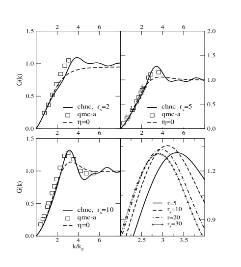
Figure 1: The local-field factors calculated from CHNC, with and without ($\eta=0$) the bridge term. The QMC data, squares, ref moroni were extracted from Davoudi et al.tosi , with the asymptotic-$k$ behaviour subtracted out (see text), and labeled ”qmc-a”. The lower right panel shows the $\sim 3k_{F}$ hump structure of the LFF for $r_{s}$=5,10,20 and 30 obtained from CHNC.

The featureless $2k_{F}$ region and the appearance of a broad hump near $3k_{F}$ are shown for $r_{s}$=5,10,20, and 30 in the lower right panel. The increased coupling (larger $r_{s}$) moves the peak to shorter wavevectors. The absence of structure near $2k_{F}$ implies a weakening of Friedel oscillations and Kohn anomalies in 2D.

Figure 2: Electron scattering across the Fermi disk. (a) Single-electron scattering. (b) Scattering of a correlated u- and d-spin pair. (c)A typical Feynman graph describing these correlations.

Discussion— The strong coupling effects in the 2DEG were modeled in CHNC via a bridge term limited to short-range interactions ( $k>2k_{F}$). This term plays a role only for anti-parallel spins, i.e., in $g_{12}(r)$. Also, available results (not discussed here) show that the hump near $3k_{F}$ does not appear for the parallel spin case (the antisymmetric LFF), where the $2k_{F}$ behaviour is similar to that expected from low-order perturbation theory. These considerations suggest that the structure near $3k_{F}$ my be a result of correlated pair processes. The broadness of the peak suggests that this is not a sharp process. The lack of Pauli exclusion between two opposite-spin electrons and the strong coupling would lead to correlated pairs. Our results show their importance in the classical fluid which is the CHNC map of the quantum fluid. Hence we make the hypothesis that such pairs play a role in the quantum liquid as well. In Fig. 2(a) an uncorrelated electron scatters with an electron across the Fermi disk, with a change of momentum $\Delta k$ = $2k_{F}$. The structure seen in the LFFs near $2k_{F}$ in weak coupling arises from such uncorrelated scattering across the Fermi disk. Although there is another electron of opposite spin in the same $k_{F}$-state, it is uncorrelated with the scattering electron and takes no part in the transition.

Consider the correlated case, Fig. 2 (b), where the up-spin $u$, and down-spin $d$ electron are in two states at $k_{F}$, making an angle $\alpha$ in the Fermi disk. If the Coulomb repulsion were absent, the $u$, $d$ pair would occupy the same state with $\alpha=0$. Unlike in the uncorrelated case (a), scattering of the correlated $u,d$ pair can occur in a concerted manner and would lead to a $\Delta k$ = $4k_{F}cos(\alpha/2)$. Depending on the correlations existing in the fluid, some optimal value of $\alpha$ would be most probable. The maxima in the LFF for $r_{s}$=5, and 20 are at $\Delta k/k_{F}$= 3.34 and $\sim 3$. This mimics the shift in In the peak in the $S(k)$ from 2.98 to 2.68 for $r_{s}$= 5 and 20. If these processes are to be treated in a diagrammatic theory for the polarization operator, then diagrams like Fig. 2 (c) are needed. The peak structure is strongest at the density $r_{s}=5.41$, where correlated singlet-pair effects are most strong. After that exchange effects begin to counter correlation effects.

At finite temperature, correlated-pair scattering should become weaker and the peak position should shift towards larger $k/k_{F}$, rather than towards 2$k_{F}$. This is confirmed in the finite-$T$ data for $r_{s}$=20 shown in Fig. 3.

Finally we remark that the bridge term ( similarly, the back-flow term in QMC) provides extra pair-interactions which make the paramagnetic fluid energetically less favourable than the ferromagnetic phase. Thus the recently proposed para$\to$ ferro transition atta ; pd2d occurs only if bridge contributions (or, in the QMC case, back-flow terms) are included in the analysis. That is, there are no para$\to$ ferro transitions in the $\eta=0$ CHNC calculation balutay .

Figure 3: Temperature ($t=T/T_{F}$) dependence of the LFF peak at $r_{s}$=20.

Conclusion— We have shown that the CHNC derived LFF provides a remarkably good representation of the quantum simulation results so far available. Unusual features of the 2D-LFF not found in the 3D-case, and unexpected from perturbation theory, were examined via the CHNC method. The lack of structure near 2$k_{F}$ and the presence of unexpected structure near 3$k_{F}$ which arises only when cluster-terms are included in the classical map suggest them to be signatures of correlated singlet-pair scattering in the 2-D electron fluid. The possibility of such scattering would be very relevant to theories of superconductivity in 2-D systems, spintronics and related topics. The CHNC method thus provides a useful exploratory tool for strongly correlated regimes inaccessible by standard analytical methods. On-line access to our CHNC codes and more details may be obtained at our websiteweb .

References

- (1) electronic mail address: chandre@nrcphy1.phy.nrc.ca NRC Visiting scientist.
- (2) A.K Rajagopal and J. C. Kimball, Phys. Rev. B 15, 2819 (1977)
- (3) K. S. Singwi,M. P. Tosi, R. H. Land, and A. Sjölander, Phys. Rev. 176 589 (1968);
- (4) N. Iwamoto, Phys. Rev. A 30, 3289 (1984)
- (5) B. Davoudi, M. Polini, G. F. Giuliani, and M. P. Tosi Phys. Rev. B 64, 153101 (2001)
- (6) J. Moreno and D. C. Marinescu, cond-mat/0206465
- (7) G. S. Atwal, I. G. Khalil and N. W. Ashcroft, Phys. Rev. B, 67 115107 (2003); I. G. Khalil, M. Teter and N. W. Ashcroft, Phys. Rev. B 65, 195309 (2002)
- (8) S. Moroni, D. M. Ceperley, and G. Senatore, as quoted in Ref. 10 of B, Davoudi et al., Ref. tosi .
- (9) M. W. C. Dharma-wardana and F. Perrot, Phys. Rev. Lett. 84, 959 (2000)
- (10) François Perrot and M. W. C. Dharma-wardana, Phys. Rev. B, 62, 16536 (2000)
- (11) François Perrot and M. W. C. Dharma-wardana, Phys. Rev. Lett. 87, 206404 (2001)
- (12) M. W. C. Dharma-wardana and F. Perrot, Phys. Rev. Lett. 90, 136601 (2003)
- (13) M. W. C. Dharma-wardana and F. Perrot, Phys. Rev. B, 66, 14110 (2002)
- (14) J. M. J. van Leeuwen, J. Gröneveld, J. de Boer, Physica 25, 792 (1959)
- (15) F. Lado, S. M. Foiles and N. W. Ashcroft, Phys. Rev. A 26, 2374 (1983)
- (16) Y. Rosenfeld, Phys.Rev. A 42, 5978 (1990), M. Baus et al., J. Phys. C: Solid State Phys. 19, L463 (1986)
- (17) G. Nicklasson, Phys. Rev. B 10, 3052 (1974), A. Holas, in Strongly Coupled Plasma Physics, Edited by F. J. Rogers and H. E. DeWitt (Plenum, New York,1987) p.463, G. Vignale and K. S. Singwi, Phys. Rev. B 32, 2156 (1985)
- (18) C. Bulutay and B. Tanatar, Phys. Rev. B 65, 195116 (2002)
- (19) M. W. C. Dharma-wardana and F. Perrot, condmat/0211127 This paper contains preliminary results from somewhat less accurate numerical procedures, partly associated with ensuring that the bridge function was truly short ranged. We find that the best way to ensure a short-ranged bridge function is to use no bridge function () up to , and then include a finite for . The cross over is quite smooth, esp. at large coupling.
- (20) Y.Kwon et al., Phys. Rev. B 48, 12037 (1993) B. Tanatar et al., Phys. Rev B 39, 5005 (1989)
- (21) Attacalite et al.,Phys. Rev. Lett.88, 256601 (2002)
- (22) http://nrcphy1.phy.nrc.ca/ims/qp/chandre/chnc