Continuous Quantum Phase Transition in a Kondo Lattice Model

Abstract

We study the magnetic quantum phase transition in an anisotropic Kondo lattice model. The dynamical competition between the RKKY and Kondo interactions is treated using an extended dynamic mean field theory (EDMFT) appropriate for both the antiferromagnetic and paramagnetic phases. A quantum Monte Carlo approach is used, which is able to reach very low temperatures, of the order of 1% of the bare Kondo scale. We find that the finite-temperature magnetic transition, which occurs for sufficiently large RKKY interactions, is first order. The extrapolated zero-temperature magnetic transition, on the other hand, is continuous and locally critical.

The observation of magnetic quantum critical points and associated non-Fermi liquid behavior has raised a renewed interest in Kondo lattice systems StewartRMP01 . An antiferromagnetic phase transition in dimensions higher than one was anticipated very early on Hewson-book93 ; Doniach77 ; VarmaNFL02 . For a spin $S={1\over 2}$ Kondo lattice system that is not too far away from half-filling, an antiferromagnetic metal phase is expected if the RKKY interactions dominate over the Kondo interactions, whereas a paramagnetic heavy fermion phase should occur in the opposite limit. Except for some special cases TsunetsuguRMP97 , however, there has been a lack of dynamical treatments of the competition between antiferromagnetism and Kondo effects in lattice problems. A key issue that has been left open is whether the zero-temperature magnetic phase transition is first order or continuous; certainly quantum critical fluctuations can be of any relevance only if the transition is either continuous or, at most, very weakly first order. This issue is generally important, but takes a particularly significant role in the context of the local quantum critical point (LQCP) Lcp-Nature01 ; GrempelSi02 . The latter has been invoked to explain some of the non-Gaussian quantum critical properties observed in the heavy fermion metals  StewartRMP01 ; Schroder00 ; Kuchler ; Aronson95 ; Questions01 .

In this paper, we study the dynamical competition between the RKKY and Kondo interactions using an extended dynamical mean field theory (EDMFT) SiSmith96 ; Chitra00 ; Spinglass . We analyze the global phase diagram of the model by carrying out EDMFT studies that cover not only the paramagnetic phase but also the antiferromagnetically ordered phase. Our analysis involves a numerical approach to the self-consistent EDMFT equations. To understand the nature of the quantum phase transition requires a study at sufficiently low temperatures, and this is in general very difficult to achieve numerically. We have overcome this difficulty by focusing on a Kondo lattice model with Ising anisotropy. We are able to reach temperatures of the order of about 1% of the bare Kondo scale, adapting a quantum Monte Carlo (QMC) methodGrempelRozenberg99 ; Grempel-QMC98 . Our most important conclusion is that the zero-temperature transition is indeed continuous and locally critical. We have also determined in some detail the dynamics in the ordered and paramagnetic phases.

The model is specified by the following Hamiltonian:

$$\mathcal{H}=\sum_{ij\sigma}t_{ij}~{}c_{i\sigma}^{\dagger}c_{j\sigma}+\sum_{i}J_{K}~{}{\bf S}_{i}\cdot{\bf s}_{c,i}+\sum_{ij}(I_{ij}/2)~{}S_{i}^{z}S_{j}^{z}.$$ (1)

Here, $c_{i\sigma}^{\dagger}$ creates a conduction electron of spin projection $\sigma$ at the $i$-th site, and ${\bf S}_{i}$ and ${\bf s}_{c,i}$ represent the spins of the $S={1\over 2}$ local moment and conduction electrons respectively; $t_{ij}$ is the hopping integral [corresponding to a band dispersion $\epsilon_{\bf k}$ ] and $J_{K}$ the Kondo coupling. The chemical potential ($\mu$) is chosen so that the system is less than half-filled; all the phases we will consider are metallic. Finally, $I_{ij}$ denote the Ising-exchange interactions between the local moments. The corresponding Fourier transform, $I_{\bf q}$, is most negative at an antiferromagnetic wavevector ${\bf Q}$ ($I_{\mathbf{Q}}=-I$). To access a LQCP, we will consider two-dimensional magnetism Lcp-Nature01 ; GrempelSi02 and take the RKKY -density-of-states in the form:

$$\rho_{I}(\epsilon)\equiv\sum_{\bf q}\delta(\epsilon-I_{\bf q})=(1/{2I})\Theta(I-|\epsilon|),$$ (2)

where $\Theta$ is the Heaviside function. In addition, we consider a featureless $\rho_{0}(\epsilon)\equiv\sum_{\bf k}\delta(\epsilon-\epsilon_{\bf k})$.

We seek to determine the transition into an antiferromagnetic state. To incorporate an order parameter, we separate the inter-site exchange interaction term into its Hartree and normal-ordered parts SiSmith96 ; Chitra00 : $\mathcal{H}_{I}=\sum_{ij}I_{ij}\left[(1/2)~{}:S_{i}^{z}::S_{j}^{z}:+\langle S_{j}^{z}\rangle S_{i}-(1/2)\langle S_{i}^{z}\rangle\langle S_{j}^{z}\rangle\right]$, where $:S_{i}^{z}:\equiv S_{i}^{z}-\langle S_{i}^{z}\rangle$. In the EDMFT mapping to a self-consistent impurity model, the first term on the RHS of $\mathcal{H}_{I}$ leads to a coupling of $:S^{z}:$ (at the selected site) to a fluctuating magnetic field. Up to constant terms, the effective impurity action takes the form:

$$\mathcal{S}_{\text{imp}} = \mathcal{S}_{\text{top}}+\int_{0}^{\beta}d\tau[h_{\text{loc}}~{}S^{z}(\tau)+J_{K}\mathbf{S}(\tau)\cdot\mathbf{s}_{c}(\tau)]$$ (3)

$$-\int\int_{0}^{\beta}d\tau d\tau^{\prime}\sum_{\sigma}c_{\sigma}^{\dagger}(\tau)G_{0,\sigma}^{-1}(\tau-\tau^{\prime})c_{\sigma}(\tau^{\prime})$$

$$-\frac{1}{2}\int\int_{0}^{\beta}d\tau d\tau^{\prime}S^{z}(\tau)\chi_{0}^{-1}(\tau-\tau^{\prime})S^{z}(\tau^{\prime})\;,$$

where $\beta=1/k_{B}T$, $\mathcal{S}_{\text{top}}$ describes the Berry phase of the local moment, and $h_{\text{loc}}$, $G_{0,\sigma}^{-1}$, and $\chi_{0}^{-1}$ are the static and dynamical Weiss fields. These fields are subject to the self-consistency condition:

$$h_{\text{loc}} = -[I-\chi_{0}^{-1}(\omega=0)]~{}m_{\text{AF}}$$ (4a)

$$\chi_{\text{loc}}(\omega) = \int_{-I}^{I}d\epsilon~{}{\rho_{I}(\epsilon)\over{M(\omega)+\epsilon}},$$ (4b)

$$G_{\text{loc},\sigma}(\omega) = \int_{-D}^{D}d\epsilon~{}{\rho_{0}(\epsilon)\over{\omega+\mu-\epsilon-\Sigma_{\sigma}(\omega)}}\;,$$ (4c)

with the aid of Dyson-like equations: $\Sigma_{\sigma}(\omega)=G_{0,\sigma}^{-1}(\omega)-\frac{1}{G_{\text{loc},\sigma}(\omega)}$, $M(\omega)=\chi_{0}^{-1}(\omega)+\frac{1}{\chi_{\text{loc}}(\omega)}$. Here $M(\omega)$ and $\Sigma_{\sigma}(\omega)$ are the spin and conduction-electron self-energies, respectively; $m_{\text{AF}}=\langle S^{z}\rangle_{\text{imp}}$ is the staggered magnetization; $\chi_{\text{loc}}(\omega)$ and $G_{\text{loc},\sigma}(\omega)$ are the Fourier transforms of $\langle T_{\tau}[:S^{z}(\tau)::S^{z}(0):]\rangle_{\text{imp}}$ and $-\langle T_{\tau}[c_{\sigma}(\tau)c_{\sigma}^{\dagger}(0)]\rangle_{\text{imp}}$, respectively. The lattice spin susceptibility is SiSmith96 :

$$\chi({\bf q},\omega)=1/[I_{\bf q}+M(\omega)]$$ (5)

The self-consistent impurity model, Eq. (3), can also be written in a Hamiltonian form,

$${\cal H}_{\text{imp}}= h_{\text{loc}}~{}S^{z}+J_{K}~{}{\bf S}\cdot{\bf s}_{c}+\sum_{p\sigma}E_{p,\sigma}~{}c_{p\sigma}^{\dagger}~{}c_{p\sigma}$$ (6)

$$+\;g\sum_{p}S^{z}\left(\phi_{p}+\phi_{-p}^{\;\dagger}\right)+\sum_{p}w_{p}\,\phi_{p}^{\;\dagger}{\phi}_{p}\;.$$

It describes a local moment coupled not only to a fermionic bath ($c_{p\sigma}$), but also to a dissipative bosonic bath ($\phi_{p}$) and a static field. Here $E_{p\sigma}$, $w_{p}$ and $g$ are such that $\sum_{p}{2w_{p}g^{2}}/(\omega^{2}-w_{p}^{2})=-\chi_{0}^{-1}(\omega)$, $\sum_{p}1/(\omega-E_{p\sigma})=G_{0,\sigma}(\omega)$. In order to understand the quantum phase transition, we need to reach sufficiently low temperatures; this is made possible by projecting Eq. (6) to a form that does not involve vastly different energy scales. For a Kondo lattice, the ordered staggered magnetization should be mostly associated with the localized moments. Its main effect in Eq. (6) is to generate, in addition to a finite $h_{\text{loc}}$, a Zeeman splitting in the fermionic bath. For featureless conduction electron density of states we are considering, however, this splitting should yield a negligible difference between the fermionic density of states at the chemical potential for the two spin species. Denoting $\sum_{p}\delta(\omega-E_{p\sigma})=N_{0}$, we can then adopt the same canonical transformation ${\cal H}_{\text{imp}}^{\prime}\equiv U^{\dagger}{\cal H}_{\rm imp}U$ within a bosonization procedure, as used in Ref. GrempelSi02 , to transform ${\cal H}_{\text{imp}}$ into

$${\cal H}_{\text{imp}}^{\prime}= h_{\text{loc}}~{}S^{z}+\Gamma S^{x}+\Gamma_{z}S^{z}s^{z}+{\cal H}_{0}$$ (7)

$$+\;g\sum_{p}S^{z}\left(\phi_{p}+\phi_{-p}^{\;\dagger}\right)+\sum_{p}w_{p}\,\phi_{p}^{\;\dagger}{\phi}_{p}\;,$$

where ${\cal H}_{0}$ describes the fermionic bath, $s^{z}$ is the $z$-component of the fermionic bath spin density, and $\Gamma$ and ${\Gamma_{z}}$ are respectively determined by the spin-flip and longitudinal components of the Kondo coupling. The corresponding partition function is $Z_{\text{imp}}^{\prime}\sim{\text{Tr}}~{}{\rm exp}[-{\cal S}_{\text{imp}}^{\prime}]$ where the trace is taken in the spin space and

$${\cal S}_{\text{imp}}^{\prime} = \int_{0}^{\beta}d\tau[h_{\text{loc}}~{}S^{z}(\tau)+\Gamma S^{x}-{1\over 2}\int_{0}^{\beta}d\tau^{\prime}S^{z}(\tau)S^{z}(\tau^{\prime})$$ (8)

$$\times(\chi_{0}^{-1}(\tau-\tau^{\prime})-{\cal K}_{c}(\tau-\tau^{\prime}))].$$

Here, ${\cal K}_{c}(i\omega_{n})=\kappa_{c}|\omega_{n}|$ ($\kappa_{c}\sim\Gamma_{z}^{2}N_{0}^{2}$) is a retarded interaction from integrating out the fermionic bath.

The effective impurity model is solved using a quantum Monte Carlo (QMC) method GrempelRozenberg99 ; Grempel-QMC98 ; GrempelSi02 . We iterate on $h_{\text{loc}}$ and $\chi_{0}^{-1}(\tau)$, through the self-consistency Eq. (4). In the following we will consider $\kappa_{c}=\pi$, and $N_{0}\Gamma=0.19$, corresponding to the bare (normalized) Kondo scale $N_{0}T^{0}_{K}=0.17$. The number of time slices in the Trotter decomposition, $N_{T}$, was chosen such as to make the discretization error small enough. We found that $N_{T}\geq 6\;\beta\;T^{0}_{K}$ is appropriate. In our simulations $N_{T}$ varied between 32 for the higher temperatures and 512 for the lowest one. We used $10^{6}$ MC steps per time slice and performed between 5 and 25 iterations.

That antiferromagnetism develops for sufficiently large RKKY interactions is seen in Fig. 1(a), which shows the temperature dependence of the staggered magnetization ($m_{\text{AF}}$) as a function of temperature at $I=3T_{K}^{0}$ and $I=1.5T_{K}^{0}$. The order parameter $m_{\text{AF}}$ becomes non-zero at $T_{\text{N}}\approx 0.29T_{K}^{0}$ and $T_{\text{N}}\approx 0.05T_{K}^{0}$, respectively. The numerical data are consistent with a jump in $m_{{\text{AF}}}$ at $T_{\text{N}}$, suggesting that the finite temperature magnetic transition is first order. This is further supported by the $T$-dependence of the static local susceptibility shown in Fig. 1(b). It is seen that $\chi_{\text{loc}}(T_{\text{N}})$ is finite whereas, for an RKKY density of states of Eq. (2), it must be divergent if the transition were second order [following arguments similar to those given after Eq. (9)] note2 .

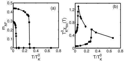
Figure 1: Temperature dependence of the staggered magnetization $m_{\text{AF}}$ (a) and the normalized static local susceptibility (b) for the values of the RKKY interaction $I/T_{K}^{0}=3.0$ (squared curves) and $1.5$ (diamond curves).

The dependence of the Néel temperature on the RKKY interaction is shown in Fig. 2(a). It is seen that $T_{\text{N}}$ vanishes at $I_{c}/T_{K}^{0}\approx 1.2$. The staggered magnetization at the lowest temperature ($T=0.011T_{K}^{0}$) also vanishes continuously at the same value $I_{c}$ as shown in Fig. 2(b). Finally, the size of the jump of $m_{\text{AF}}$ at $T_{\text{N}}$ decreases with the latter as the strength of the RKKY interaction is reduced. The extrapolated value of the jump also goes to zero at $I_{c}$. These observations strongly suggest that the zero-temperature transition is second order.

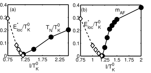
Figure 2: (a) The Néel temperature (solid dots) and $E_{\text{loc}}^{*}$ (open diamonds) as a function of $I/T_{K}^{0}$, the ratio of the RKKY interaction to the bare Kondo scale; (b) The staggered magnetization (solid dots) as a function of of $I/T_{K}^{0}$, at $T=0.011T_{K}^{0}$. $E_{\text{loc}}^{*}$ characterizes the coherence scale of the paramagnetic solution (see the main text). The solid and dashed lines are guides to eyes.

We also show in Fig. 2 $E_{\text{loc}}^{*}$, the coherence scale of the Kondo lattice as a function of $I$. It may be seen that $E_{\text{loc}}^{*}$ is finite for $I<I_{c}$ but decreases with increasing $I$; within our numerical uncertainty, it vanishes precisely at $I_{c}$. $E_{\text{loc}}^{*}$ characterizes the crossover from the low energy Fermi liquid regime, in which the local susceptibility has a Pauli form, to the high energy quantum critical regime where the local susceptibility is logarithmically singular. This scale is determined numerically from the frequency dependence of the local susceptibility as discussed in Ref. GrempelSi02 . In this range ($I<I_{c}$), the solution derived from starting the iteration with a zero trial $h_{\text{loc}}$ is identical to that with a finite trial $h_{\text{loc}}$. That the values of $I_{c}$ determined from the paramagnetic and ordered sides are the same provides an additional evidence for the second order nature of the quantum phase transition.

We wish to stress a subtle issue in the determination of $I_{c}$ coming from the paramagnetic side. If we apply the paramagnetic EDMFT equations (i.e., with $h_{\text{loc}}=0$) to $I>I_{c}$, we find that they would converge to a nominally “paramagnetic” solution (at least for $I\leq 3T^{0}_{K}$). These solutions are, however, characterized by free residual (but not ordered!) moments, as signaled by a ${\cal C}/T$ divergence in $\chi_{\rm loc}(T)$ at low temperatures; the constant ${\cal C}$ is an effective Curie constant. This Curie constant manifests also in the behavior of $\chi_{\text{loc}}(\omega_{n})$ at $\omega_{n}=0$, as illustrated (for a particular value $I=2T_{K}^{0}\gg I_{c}$) in the inset to Fig. 3: $\chi_{\text{loc}}(\omega_{n}=0)$ jumps by an amount ${\cal C}/T$ compared to the value extrapolated from $\chi_{\text{loc}}(\omega_{n})$ at finite $\omega_{n}$ note . (Without going to low temperatures, this jump would have been hard to see.) From the dependence of ${\cal C}$ on $I$ (Fig. 3, main plot), the Curie constant is seen to vanish as $I$ approaches $I_{c}$ from above. The finite Curie constant for all $I>I_{c}$ shows that, in this region, the nominally “paramagnetic” solution is unstable and the true ground state is the antiferromagnetic solution.

Figure 3: Curie constant ${\cal C}$ in the nominally “paramagnetic” solution as a function of $I/T_{K}^{0}$. Inset: the local susceptibility vs. Matsubara frequency $\omega_{n}$ for $I=2T_{K}^{0}$ at various temperatures; the jump at $\omega_{n}=0$ measures ${\cal C}/T$.

That $E_{\text{loc}}^{*}$ has to vanish at $I_{c}$ can in fact be understood once the continuous onset of $T_{\text{N}}$ and $m_{\text{AF}}$ at $I_{c}$ is established. A second order magnetic transition at zero temperature means that $\chi({\bf Q},\omega=0,T=0)$ diverges at $I_{c}$. Using

$$\chi({\bf Q},\omega=0,T=0)=1/[M(\omega=0,T=0)-I]$$ (9)

[which can be seen by inserting $I_{\bf Q}=-I$ into Eq. (5)], this implies that $M(\omega=0,T=0)=I$. It then follows from the self-consistency Eq. (4b), together with Eq. (2), that the local susceptibility $\chi_{\text{loc}}(\omega=0,T=0)$ also diverges note2 at $I=I_{c}$. This places the local Kondo problem, as specified by Eq. (6) with $h_{\text{loc}}=0$, to be at its own critical point note2 . In other words, the criticality of the Kondo physics is embedded in the criticality of the magnetic transition in the lattice; the corresponding coherence energy scale, $E_{\text{loc}}^{*}$, vanishes.

The overall phase diagram is now specified by Fig. 2(a). While the first order nature of the finite temperature transition is an artifact of EDMFT, reflecting the fact that EDMFT contains no spatial anomalous dimension, the LQCP at zero temperature is expected to be robust Lcp-Nature01 ; note2 . By establishing the continuous nature of the zero-temperature transition, we can identify a finite-temperature quantum-critical “fan” that is anchored by the ($T=0$) LQCP at $I=I_{c}$, even in the absence of a correct understanding of the finite temperature transition. This quantum critical fan can be used to describe the non-Gaussian quantum critical behavior observed in heavy fermion metals.

To better understand the dynamics in the ordered phase, we have also calculated the frequency dependence of the local susceptibility. Fig. 4 plots $\chi_{\text{loc}}(\omega_{n})$ vs $\omega_{n}$ for various values of $I/T_{K}^{0}$, at $T=0.011T_{K}^{0}$. On the ordered side, the peak susceptibility, $\chi({\bf Q},\omega_{n})$, saturates to a finite value as a result of the finite magnetic order parameter. Correspondingly, the local susceptibility, $\chi_{\text{loc}}(\omega_{n})$, which is equal to the ${\bf q}$-average of $\chi({\bf q},\omega_{n})$, also saturates. The saturated value of $\chi_{\text{loc}}(\omega_{n})$ increases as the RKKY interaction and, correspondingly, $h_{\text{loc}}$, is reduced. At $I=I_{c}\approx 1.2T_{K}^{0}$, $h_{\text{loc}}$ goes to zero and the local susceptibility becomes logarithmically singular, the form that is associated with the critical point of this self-consistent impurity model; the result at $I=I_{c}$ agrees with that of the analysis from the paramagnetic side.

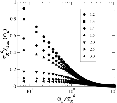
Figure 4: The normalized local susceptibility vs. Matsubara frequency, at $T=0.011T_{K}^{0}$. The legend specifies $I/T_{K}^{0}$.

One of us (JXZ) acknowledges the useful discussions with A. V. Balatsky, Y. Bang and L. Zhu, and the hospitality of Rice University, where part of the research was carried out. This work has been supported by US DOE (JXZ), NSF at KITP (DRG) and NSF, the Welch Foundation and TCSAM (QS). It was first reported in Ref. APS03 . We have recently learned that P. Sun and G. Kotliar Sun03 have independently addressed similar issues in an Anderson lattice at high temperatures.

References

- (1) G. R. Stewart, Rev. Mod. Phys. 73, 797 (2001).
- (2) A. C. Hewson, The Kondo Problem to Heavy Fermions (Cambridge Univ. Press, Cambridge, 1993).
- (3) S. Doniach, Physica B 91, 231 (1977).
- (4) C. M. Varma, Rev. Mod. Phys. 48, 219 (1976).
- (5) H. Tsunetsugu et al., Rev. Mod. Phys. 69, 809 (1997).
- (6) Q. Si et al., Nature 413, 804 (2001); Phys. Rev. B 68, 115103 (2003).
- (7) D. R. Grempel and Q. Si, Phys. Rev. Lett. 91, 026401 (2003).
- (8) A. Schröder et al., Nature 407, 351 (2000).
- (9) R. Küchler et al., Phys. Rev. Lett. 91, 066405 (2003)
- (10) M. C. Aronson et al., Phys. Rev. Lett. 75, 725 (1995).
- (11) P. Coleman et al., J. Phys. Cond. Matt. 13, R723 (2001).
- (12) Q. Si and J. L. Smith, Phys. Rev. Lett. 77, 3391 (1996); J. L. Smith and Q. Si, Phys. Rev. B 61, 5184 (2000).
- (13) R. Chitra and G. Kotliar, Phys. Rev. Lett. 84, 3678 (2000); H. Kajueter, Ph.D. thesis Rutgers Univ. (1996).
- (14) Related approaches with a particular form of self-consistency appear in other contexts: J. Ye, S. Sachdev, and N. Read, Phys. Rev. Lett. 70, 4011 (1993); A. M. Sengupta and A. Georges, Phys. Rev. B 52, 10295 (1995); A. J. Bray and M. A. Moore, J. Phys. C13, L655 (1980).
- (15) D. R. Grempel and M. J. Rozenberg, Phys. Rev. B 60, 4702 (1999).
- (16) D. R. Grempel and M. J. Rozenberg, Phys. Rev. Lett. 80, 389 (1998); M. J. Rozenberg and D. R. Grempel, ibid. 81, 2550 (1998).
- (17) Both a finite and a divergent are compatible with the fact that , being also determined by an effective impurity model, must be finite at any finite but can diverge at . In general, for a () LQCP a vanishing spatial anomalous dimension is internally consistent Lcp-Nature01 so our results should be robust beyond EDMFT. A classical critical point, on the other hand, usually has a finite and is not correctly described by EDMFT.
- (18) The solution with and a finite Curie constant at can be understood as follows. A term in implies an extra term in the Weiss field of the form , where is positive. The solution for to such an Ising Bose-Fermi Kondo model Zhu02 contains connected and disconnected pieces; self-consistently, the two pieces determine the Curie constant and regular part of , respectively.
- (19) L. Zhu and Q. Si, Phys. Rev. B 66, 024426 (2002); G. Zaránd and E. Demler, ibid., 024427 (2002).
- (20) J.-X. Zhu, D. R. Grempel, and Q. Si, Bull. Am. Phys. Soc. 48(1), 827 (2003)[March].
- (21) P. Sun and G. Kotliar, cond-mat/0303539. Detailed comparison between the two works is not easy to make, since the models are different and, in addition, the covered temperature ranges barely overlap.