ARPES and optical renormalizations: phonons or spin fluctuations

Abstract

Improved resolution in both, energy and momentum in ARPES-data has lead to the establishment of a definite energy scale in the dressed quasiparticle dispersion relations. The observed structure around $80\,$meV has been taken as evidence for coupling to phonons and has re-focused the debate about the mechanism of superconductivity in the cuprates. Here we address the relative merits of phonon as opposed to spin fluctuation mechanisms. Both possibilities are consistent with ARPES. On the other hand, when the considerations are extended to infrared optical data, a spin fluctuation mechanism provides a more natural interpretation of the combined sets of data in Bi₂Sr₂Ca Cu₂O_8+δ (Bi2212).

I Introduction

With the advent of improved resolution, both in energy and momentum, several angular resolved photo emission spectroscopy (ARPES) groups have measured the renormalized quasiparticle energies and/or lifetimeskaminski ; valla ; johnson ; kaminski1 ; lanzara ; bogdanov ; valla1 ; valla2 in the cuprates. The data shows that a definite energy scale exists for the renormalization. This energy scale has tentatively been assigned by somelanzara ; bogdanov to interactions of the charge carriers with phonons. This provocative possibility has again brought to the forefront the open question of mechanism in the cuprates and in particular the possibility that the electron-phonon interaction plays an important role. While the electron-phonon interaction is widely believed to cause superconductivity in conventional materials, the gap symmetry in the cuprates is $d$-wavemars6 ; hardy ; shen ; wollm ; tsuei rather than $s$-wave which means that it is the projection of the electron phonon interaction on the $d$-channel which enters the equation for the critical temperature $T_{c}$. This would imply that some of the details of the electron-phonon interaction would be drastically different in the oxides compared to conventional metals. While conventional superconductors do exhibit anisotropytomlinson ; carb2 in their superconducting gap as a function of momentum k on the Fermi surface, the $s$-channel always overcomes the $d$-channel interaction. Also in dirty $s$-wave materials with the mean free path $\ell$ smaller than the coherence length $\xi_{0}$, the anisotropy is washed out and the gap becomes isotropic. On the other hand, in the pure limit there are many ways in which this gap anisotropy manifests itself in a conventional superconductor.carb2 One example is the low temperature $(T)$ electronic specific heat which exhibits the expected exponential dependence $\exp\{-\Delta/T\}$ only for temperatures much lower than the lowest gap $(\Delta)$ in the system.

Arguments for why the form of the electron-phonon interaction can be very different in the oxides as compared with conventional metals have been presented in the literature. Some of the critical ideas have been reviewed by Kulić.no15 The main argument for our purpose here is that the electron-phonon interaction becomes strongly peaked in the forward direction when corrections for strong correlations are properly accounted for through charge vertices.zeyher ; kulic Another related idea is that because of the large static dielectric function in the oxides the screening is greatly reduced as compared with ordinary metals. This also leads to enhanced forward scattering as can be seenweger ; weger1 from the following simple argument. The Fourier transform of the bare Coulomb potential diverges like $1/q^{2}$ for small q, here q is the momentum transfer. Screening eliminates this singularity and the screened potential goes, instead, like $1/(q^{2}+\lambda^{2}_{\rm FT})$, where $\lambda_{\rm FT}$ is an inverse screening length. For small $\lambda_{\rm FT}$ the increased forward scattering has the general tendency of increasing the weighting of the higher harmonics in its expansion. For example the expansion of a delta function $\delta({\bf q})$ has equal weight in each spherical harmonics.kulic1 Strong forward scattering can in fact lead to $d$-wave superconductivity which is not suppressed by the strong Coulomb repulsion in contrast to the $s$-wave channel.kulic1 ; kulic2

While the possibility of phonon induced $d$-wave superconductivity cannot be eliminated on general grounds, it has not been favored in much of the literature. While there is no consensus on mechanism, many workers believe instead in an electronically driven scenario: for instance, the $t-J$ model can exhibit superconductivity.sorella A spin fluctuation mechanism, such as is envisaged in the Nearly Antiferromagnetic Fermi Liquid (NAFFL) model of Pines and coworkerspines1 ; pines2 is also electronic in nature with the exchange of spin fluctuations rather than phonons. Another electronic mechanism is the Marginal Fermi Liquid (MFL) modelvarma1 ; varma2 ; varma3 which in its original form had $s$-wave symmetry.

In this paper we attempt to understand the renormalization effect observed in ARPES within a boson exchange mechanism. We will consider explicitly both, phonon and spin fluctuation exchange. We will also try to reconcile within the same model, both, ARPES data on equilibrium quasiparticle properties and the optical conductivity. Infrared measurements in the cuprates have produced a wealth of information on charge dynamics in the oxides.puchkov ; timusk They have played a key role in our present understanding of the microscopic nature of the cuprates. In particular, $c$-axis infrared conductivity data have given detailed spectroscopic information on the pseudogaptimusk which has been widely viewed as a direct manifestation of strong correlation effects. Recently, improvements in resolution have also been achieved in $ab$-plane measurements.tu

From reflectance measurements as a function of frequency it is possible to extract separately the real and the imaginary part of the conductivity $\sigma(T,\omega)$ as a function of $\omega$ for a fixed temperature $T$. Within a generalized Drude model, in which the optical scattering rate and optical effective mass acquire a frequency dependence, we can define an isotropic optical scattering time $\tau_{op}(T,\omega)$ as $\tau^{-1}_{op}=(\Omega^{2}_{p}/4\pi)\Re{\rm e}\sigma^{-1}(T,\omega)$, where $\Omega_{p}$ is the plasma frequency. This quantity can be determined from the optical sum rule on the real part of $\sigma(T,\omega)$, namely $\int_{0}^{\infty}d\omega\sigma_{1}(T,\omega)=(\Omega^{2}_{p}/8)$. The optical scattering rate defined above is related to the quasiparticle lifetime which may be considered to be more fundamental as they directly define quasiparticle motion. While these two lifetimes are related, they are by no means identical, however, except for a simplified case of isotropic elastic impurity scattering. Even in this case, if the electronic density of states has an important dependence on energy or the elastic scattering is anisotropic, quasiparticle and transport scattering rates are no longer the same. Note that, in as much as the in-plane conductivity is isotropic, the optical scattering rate is also isotropic and represents a weighted average of the more fundamental momentum dependent quasiparticle scattering. While there have been some attempts in the literaturekaminski to compare both sets of data, i.e.: ARPES and optical directly, we will emphasize here that, because they are not so simply related, they cannot easily be compared. On the other hand, any viable microscopic model needs to be able to provide a unifying description of both sets of experiments. In this regard, we will emphasize that in addition to the differences between quasiparticle and transport scattering rate which we have already discussed, they differ in another fundamental way. In a boson exchange mechanism the charge carrier-exchange boson spectral density (denoted by $\alpha^{2}F(\omega)$ in the explicit case of phonons) which describes the equilibrium properties can be quite different from the corresponding transport spectral density, usually denoted by $\alpha^{2}_{tr}F(\omega)$.tomlinson1 ; leung The origin of this fundamental difference lies in a well-known factor $(1-\cos\theta)$, where $\theta$ is the angle between initial and final electron momentum undergoing a scattering process. For quasiparticle properties such as its lifetime, only the probability that an electron of momentum k leaves the state $|{\bf k}\rangle$ is relevant, while for transport, for instance for the d.c. resistivity, it is also important where it ends up since backward scattering depletes the current more than forward scattering. This basic physics is accounted for by the $(1-\cos\theta)$ factor which eliminates forward scattering $(\theta=0)$ and weights with a factor two backward scattering $(\theta=\pi)$. Serious estimatesno15 ; zeyher ; kulic of these two spectral densities for a model electron-phonon interaction in the poor screening regime with explicit inclusion of correlation effects, have lead to an estimate that $\alpha^{2}_{tr}F(\omega)$ may be smaller by about a factor of $1/3$ compared with $\alpha^{2}F(\omega)$, the corresponding quasiparticle quantity. On the other hand, in the NAFFL model the interaction with spin fluctuations is believed to strongly peak around $(\pi,\pi)$ in momentum. This means that the scattering potential itself weights more strongly the backward scattering processes, and so we expect that the transport spectral density will be larger than its quasiparticle counterpart. The above arguments immediately suggest that phonons effects could very well show up prominently in quasiparticle properties while at the same time play only a minor role in transport, i.e.: in the infrared conductivity and vice versa for spin fluctuations.

In section II we make general remarks about the renormalization effects due to boson exchange mechanisms based on perturbation theory. In particular we contrast the electron-phonon case with spin fluctuations. In section III we deal with fits to the ARPES data in Bi2212 and in section IV we consider, in addition, optical conductivity data. We describe the constraints on microscopic models that a fit to both sets of data imposes in the specific case of Bi2212. In section V we draw conclusions.

II General results

For an electron-phonon system, the renormalization of the electronic quasiparticles follows from a knowledge of the electron-phonon spectral density $\alpha^{2}F(\omega)$. This function which depends only on frequency, and which is limited in range to the maximum phonon frequency, contains all of the complicated information about electronic band wave functions, dispersion relation, phonon dynamics, and electron-lattice vibration coupling which is needed to compute self energy effects. In lowest order perturbation theory, the quasiparticle scattering rate $\tau^{-1}_{qp}(\omega)$ at energy $\omega$ is given byallen

$$\tau^{-1}_{qp}(\omega)=2\pi\int\limits_{0}^{\omega}\!d\nu\,\alpha^{2}F(\nu).$$ (1)

For a $\delta$-function Einstein phonon at $\omega_{E}$ of the form $\alpha^{2}F(\omega)=A\delta(\omega-\omega_{E})$

$$\tau^{-1}_{qp}(\omega)=\left\{\begin{array}[]{rl}2\pi A&\omega>\omega_{E}\\ 0&\omega<\omega_{E},\end{array}\right.$$ (2)

and we see that $\omega_{E}$ sets the energy at which $\tau^{-1}_{qp}(\omega)$ jumps from zero to a finite value. For an $\alpha^{2}F(\omega)$ distributed in energy, the rise will be more gradual but for $\omega\geq\omega_{D}$, with the Debye energy $\omega_{D}$, the scattering rate will, again, become constant.

The expression for the optical scattering rate, on the other hand, which is also obtained in lowest order perturbation theory isallen

$$\tau^{-1}_{op}(\omega)={2\pi\over\omega}\int\limits_{0}^{\omega}\!d\nu\,(\omega-\nu)\alpha^{2}_{tr}F(\nu),$$ (3)

which gives $\tau^{-1}_{op}(\omega)=0$ for $\omega\leq\omega_{E}$ in an Einstein model, but now for $\omega>\omega_{E}$

$$\tau^{-1}_{op}(\omega)=2\pi\left(1-\frac{\omega_{E}}{\omega}\right)A_{tr},$$ (4)

which starts at zero with $\omega=\omega_{E}$ and gradually increases towards $2\pi A_{tr}$ with increasing $\omega$. This is quite distinct from the abrupt jump to $2\pi A$ at $\omega=\omega_{E}$ found for the quasiparticle scattering rate. Here the subscript ‘$tr$’ denotes transport as opposed to equilibrium properties. It is clear that the singularity in $\tau^{-1}(\omega)$ associated with the boson energy scale $\omega_{E}$ is more significant in the quasiparticle (equilibrium case) than in the transport scattering rate. There is yet another difference between quasiparticle and transport rates. If we denote the electron-phonon interaction matrix element by $g_{{\bf k},{\bf k}^{\prime},\nu}$ for electrons scattering from k to ${\bf k}^{\prime}$ with a phonon of energy $\omega_{\nu}({\bf k}-{\bf k}^{\prime})$ ($\nu$ is a branch index) the quasiparticle spectral density isgrimvall ; carb1 ; mars6

$$\alpha^{2}F(\omega)=\sum\limits_{\nu}\left\langle\left\langle\left|g_{{\bf k},{\bf k}^{\prime},\nu}\right|^{2}\delta(\omega-\omega_{\nu}({\bf k}-{\bf k}^{\prime}))\right\rangle\right\rangle,$$ (5)

with the double average over the Fermi surface denoted by $\left\langle\left\langle\cdots\right\rangle\right\rangle$

$$\left\langle\left\langle G\right\rangle\right\rangle=\frac{\sum\limits_{{\bf k},{\bf k}^{\prime}}G_{{\bf k},{\bf k}^{\prime}}\delta(\varepsilon_{\bf k}-\mu)\delta(\varepsilon_{{\bf k}^{\prime}}-\mu)}{\sum\limits_{\bf k}\delta(\varepsilon_{\bf k}-\mu)},$$ (6)

where $\mu$ is the chemical potential, so all integrals are pinned at the Fermi surface. The optical spectral weight is relatedtomlinson ; leung ; grimvall instead to

$$\alpha^{2}_{tr}F(\omega)\propto\sum\limits_{\nu}\left\langle\left\langle\left|g_{{\bf k},{\bf k}^{\prime},\nu}\right|^{2}\left(v_{\bf k}-v_{{\bf k}^{\prime}}\right)^{2}\delta(\omega-\omega_{\nu}({\bf k}-{\bf k}^{\prime}))\right\rangle\right\rangle.$$ (7)

The extra factor of $v_{\bf k}-v_{{\bf k}^{\prime}}$ with $v_{\bf k}$ the velocity of the electron k weights forward scattering by zero and emphasizes most backward collisions.

The functions $\alpha^{2}F(\omega)$ of Eq. (5) and $\alpha^{2}_{tr}F(\omega)$ of Eq. (7) are isotropic, momentum averages, given by the right hand side of each of these equations. Both involve a double integral over initial and final states $|{\bf k}\rangle$ and $|{\bf k}^{\prime}\rangle$. The full complicated momentum dependence of the electron-phonon coupling $g_{{\bf k},{\bf k}^{\prime},\nu}$ and of the phonon dispersion $\omega_{\nu}({\bf k}-{\bf k}^{\prime})$ is included with no approximations, although after the double summation over momentum, indicated in Eq. (6), $\alpha^{2}F(\omega)$ is now isotropic, dependent only on frequency. This is the function that enters isotropic Eliashberg theory. An anisotropic formulation of the Eliashberg equationsdaams also exists and in this case a directional electron-phonon spectral density distinct for each electron state $|{\bf k}\rangle$ on the Fermi surface, which we denote by $\alpha^{2}_{\bf k}F(\omega)$, would replace its Fermi surface average:

$$\alpha^{2}F(\omega)=\frac{\sum\limits_{\bf k}\alpha^{2}_{\bf k}F(\omega)}{\sum\limits_{\bf k}\delta(\varepsilon_{\bf k}-\mu)}.$$ (8)

To calculate $\alpha^{2}F(\omega)$ from first principles is difficult and complex.carb1 It can, fortunately, be measured directly from tunneling data through consideration of current voltage characteristics.mcmillan ; mcmillan1 The resulting function of $\omega$ often, but not always, looks qualitatively very much like the phonon frequency distribution $F(\omega)$ but this does not imply that momentum dependence of coupling and/or of phonons is not included in Eq. (5). Any nesting effects such as are present in the nested Fermi liquid theory of Virosztek and Ruvaldsru1 ; ru2 and in the work of Savrasov and Andersensavr are fully incorporated on the right hand side of Eq. (5). It is only because we take the left hand side from experiment that these important issues do not become prominent in our work.

A further complication arises in the case of coupling to spin fluctuations.branch In this case the magnetic spin susceptibility $\chi_{{\bf k},{\bf k}^{\prime}}(\omega)$ is involved as well as its coupling to charge. The susceptibility in the cuprates is sharply peaked in momentum space at the antiferromagnetic wave vector ${\bf k}-{\bf k}^{\prime}$ (momentum transfer) for electron scattering from $|{\bf k}\rangle$ to $|{\bf k}^{\prime}\rangle$. In this case, what enters Eliashberg theorybranch is the complex function $\chi_{{\bf k},{\bf k}^{\prime}}(\omega)$ weighted by electron coupling. For instance, in the NAFFL modelpines1

$$\chi_{{\bf k},{\bf k}^{\prime}}(\omega)={\chi_{\bf Q}\over 1+\xi^{2}({\bf q}-{\bf Q})^{2}-i{\omega\over\omega_{MMP}}},\quad q_{x},\,q_{y}>0,$$ (9)

with ${\bf q}={\bf k}-{\bf k}^{\prime}$, $\chi_{\bf Q}$ the static susceptibility, $\xi$ the magnetic coherence length, ${\bf Q}=(\pi,\pi)$ the commensurate antiferromagnetic momentum, and $\omega_{MMP}$ the characteristic energy of the spin fluctuations at the point Q. A Fermi surface to Fermi surface approximation does not naturally reveal itself since this may not include transitions with ${\bf k}-{\bf k}^{\prime}=(\pi,\pi)$ for which the susceptibility is the largest. However, one can still introduce, as an approximation, some average effective electron-spin fluctuation spectral function denoted by $I^{2}\chi(\omega)$ which can be used in the isotropic version of the Eliashberg equations. It represents the appropriate average of the susceptibility that enters superconductivity. Its value is to be determined from consideration of experimental data. As described by Carbotte et al.schach4 this isotropic spectral density is given by the second derivative of $\omega$ times the optical scattering rate $\tau_{op}^{-1}(\omega)$. Recall, $\tau_{op}^{-1}(\omega)=(\Omega_{p}^{2}/4\pi)\Re{\rm e}\sigma^{-1}(\omega)$, where $\sigma(\omega)$ is the in-plane optical conductivity. This conductivity is isotropic in tetragonal systems. For the orthorhombic case, $\sigma(\omega)$ with ${\bf E}\parallel a$ and ${\bf E}\parallel b$ can be different. Defining

$$W(\omega)={1\over 2\pi}{d^{2}\over d\omega^{2}}\left(\frac{\omega}{\tau_{op}(\omega)}\right),$$ (10)

the approximate relation $I^{2}_{tr}\chi(\omega)\simeq W(\omega)$ holds.mars4 We emphasize that in terms of microscopic theory $W(\omega)$ is related to an appropriate average of the full momentum and energy spin susceptibility $\chi_{{\bf k},{\bf k}^{\prime}}(\omega)$ (Eq. (9)). Recently, infrared optical data has been used very effectively to obtain $I^{2}_{tr}\chi(\omega)$ in the oxides and we will use these in our work.schach4 ; schach7 ; schach5 ; schach8 In this way we circumvent all of the complications that would arise in a first principle calculation of the average effective function $I^{2}_{tr}\chi(\omega)$. We will return to this important point later in equation (13). We note in passing that $W(\omega)$ very often exhibits a pronounced resonance like structure particularly if $\tau^{-1}_{op}(\omega)$ data at low temperatures in the superconducting state is analyzed. In the following we use the expression ‘optical resonance’ in reference to such a structure. In most materials analyzed so far, this optical resonance has a spin resonance equivalent measured using inelastic neutron scattering. We will discuss this in more detail in Sec. IV.

In some sense the opposite extreme to the NAFFL model of Pines and coworkerspines1 ; pines2 in which the interaction peaks at $(\pi,\pi)$ is the MFL model of Varma et al.varma1 ; varma2 ; varma3 in which the interaction with the fluctuation spectrum is thought of as momentum independent in a first approximation. As originally conceived, this model leads to an $s$-wave superconducting gap rather than $d$-wave as is now generally believed to be the case. This represents a real limitation for the model. Nevertheless, it has been very useful in correlating much data on the normal state transport properties in the cuprates.

In as much as it is only the magnitude and energy dependence of the resulting average spectral function $\alpha^{2}F(\omega)$ ($I^{2}\chi(\omega)$) that matter, these may not be very different between the MFL and NAFFL models. Both have an average spectral density which is reasonably flat as a function of energy and which extends to some high frequency of order several hundred meV. Of course, if anisotropies on the Fermi surface were to be considered, the directional $\alpha^{2}_{\bf k}F(\omega)$ ($I^{2}_{\bf k}\chi(\omega)$), Eq. (8), would be expected to vary strongly in the NAFFL model and not in the MFL model, but here, for simplicity, we have assigned to each electron the same average interaction. For phonons in conventional metals the mass renormalization parameter $\lambda_{\bf k}=2\int_{0}^{\infty}\!d\omega\,\alpha^{2}_{\bf k}F(\omega)/\omega$ can vary by several tens of percentage points over the Fermi surface.carb2 For the NAFFL model based on the susceptibility (9), the variations are much larger, and can be of the order of a factor of two or three.branch It is clear that ARPES data in a particular direction could considerably under or overestimate the average renormalizations. In this sense optics is better.

We should make one further remark. In conventional materials for which $\alpha^{2}F(\omega)$ and $\alpha^{2}_{tr}F(\omega)$ have been calculated from band structure and phonon information usually obtained by inelastic neutron scattering, they have been found to differtomlinson ; carb2 ; tomlinson1 ; leung in shape as a function of $\omega$ and in size. But these differences have often been overlooked in the literature. In the work of Kulić and Zeyher no15 ; zeyher ; kulic the corresponding differences are large. These authors considered directly the cuprates and try to account seriously for the ionicity and the increased effect of correlations. As described in the introduction, they find that the electron-phonon interaction in this case is strongly peaked in the forward direction and this leads to large differences between $\alpha^{2}F(\omega)$ and $\alpha^{2}_{tr}F(\omega)$. They estimate $\alpha^{2}F(\omega)$ to be about a factor of three larger than $\alpha^{2}_{tr}F(\omega)$. The consequence of this is that phonons would show up much more prominently in quasiparticle properties (equilibrium) than in the corresponding transport property. In particular, at large $\omega$, $\tau^{-1}_{qp}(\omega)$ and $\tau^{-1}_{op}(\omega)$ (Eqs. (2) and (4), respectively) would approach each other if $\alpha^{2}F(\omega)$ and $\alpha^{2}_{tr}F(\omega)$ were identical, but in fact $\tau^{-1}_{op}(\omega)$ is expected to be larger than $\tau^{-1}_{qp}(\omega)$. The opposite would hold for the NAFFL model which emphasizes backward rather than forward scattering because the interaction peaks at $(\pi,\pi)$. In this case spin fluctuations should show up more prominently in transport than in equilibrium properties. Even though these differences are hard to quantify, the general qualitative features of transport as compared with quasiparticle spectral weight just described must be kept in mind when analyzing data. In the MFL model we expect smaller differences between quasiparticle and transport spectral densities because the underlying interaction is assumed to be approximately momentum independent.

So far we have only discussed scattering rates and have emphasized the differences and similarities between infrared optical absorption and quasiparticle lifetimes. In ARPES the dressed electronic dispersion relation is measured and denoted by $E_{\bf k}$. It is related to the bare band dispersion $\varepsilon_{\bf k}$ through the electron self energy. In the electron-phonon case with an Einstein phonon spectrum and at $T=0$ (zero temperature) the self energy reduces to a simple form

$$\Sigma(\omega+i0^{+})=\frac{\lambda\omega_{E}}{2}\left[\ln\left|\frac{\omega_{E}-\omega}{\omega_{E}+\omega}\right|-i\pi\theta(\omega-\omega_{E})\right].$$ (11)

In Eq. (11) $\lambda$ is the electron mass enhancement parameter defined as $m^{\ast}/m=1+\lambda$ where $m^{\ast}$ is the renormalized electron mass at the Fermi surface. In terms of $\alpha^{2}F(\omega)$, $\lambda=2\int_{0}^{\infty}d\nu\,\alpha^{2}F(\nu)/\nu=2A/\omega_{E}$ for the simplified Einstein case. The imaginary part of Eq. (11) just gives back $\tau^{-1}_{qp}(\omega)=-2\Im{\rm m}\Sigma(\omega+i0^{+})$ of Eq. (3). The real part gives the renormalized energies as solutions of equation $E_{\bf k}=\varepsilon_{\bf k}+\Re{\rm e}\Sigma(E_{\bf k})$ and for $\varepsilon_{\bf k}\to 0$ (on the Fermi surface) this gives $E_{\bf k}=\varepsilon_{\bf k}/(1+\lambda)$: the quasiparticle mass is simply renormalized to $m^{\ast}$. Note that in Eq. (11) the self energy has a logarithmic divergence at $\omega=\omega_{E}$ and this leads to a singular structure in $E_{\bf k}$ at that energy as has been investigated in detail by Verga et al.verga to which the reader is referred for details. Here we have chosen to emphasize instead the nature of the structure in the imaginary part. It is sufficient to remark that for a finite distribution of phonon energies in $\alpha^{2}F(\omega)$ the logarithmic singularity is moderated as it also is when temperature $(T)$ is included. In the general case, $\Re{\rm e}\Sigma(\omega+i0^{+})$ takes the form

$$\Re{\rm e}\Sigma(\omega+i0^{+}) = -\int\limits_{0}^{\infty}\!d\nu\,\alpha^{2}F(\nu)\Re{\rm e}\left[\psi\left(\frac{1}{2}+i\frac{\nu-\omega}{2\pi T}\right)\right.$$ (12)

$$-\left.\psi\left(\frac{1}{2}-i\frac{\nu-\omega}{2\pi T}\right)\right],$$

where $\psi(z)$ is the digamma function. In lead, the electron-phonon spectral density $\alpha^{2}F(\omega)$ is well known from tunneling spectroscopytomlinson ; carb1 ; mcmillan ; mcmillan1 as well as from direct calculations. It is shown as an insert in the top frame of Fig. 1.

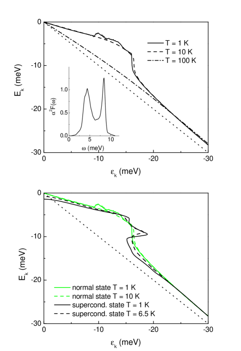
Figure 1: Top frame: the renormalized energies $E_{\bf k}$ in lead as a function of the bare band energy $\varepsilon_{\bf k}$; the renormalization is due to the electron phonon interaction characterized by the electron-phonon spectral density $\alpha^{2}F(\omega)$ shown in the inset. The bare dispersion is shown as the dotted line. The other curves are for the normal state at $T=1\,$K (solid), $T=10\,$K (dashed), and $T=100\,$K (dash-dotted). Bottom frame: same as the top frame but for the superconducting state at $T=1\,$K (solid) and $T=6.5\,$K (dashed) just below $T_{c}=7.2\,$K. The normal state results are shown as gray lines for comparison.

The phonons extend to $12\,$meV and show a characteristic peak for transverse and for longitudinal branches. In the top frame of this figure we show numerical results in the normal state for $E_{\bf k}$ on the Fermi surface as a function of the bare band electronic energy $\varepsilon_{\bf k}$ up to $30\,$meV at which point bare (dotted curve) and renormalized energies are pretty well parallel to each other. The solid curve applies to the normal state at $T=1\,K$. We see structure in the renormalized quasiparticle energy $E_{\bf k}$ ranging up to roughly $10\,$meV. The structure clearly corresponds to the structure in the phonon spectrum (inset). Beyond this range multi-phonon processes are operative and the renormalization effects are less. Further results in the normal state are for $T=10\,$K (dashed) and $T=100\,$K (dash-dotted). We see that by the time this last temperature is reached, which is of the order of the maximum phonon energy, the thermal effects have smeared out much of the structure. Note also, that in all three cases the curves go through zero at $\varepsilon_{\bf k}=0$ and the slope of each line out of the origin gives the renormalized effective mass parameter $(1+\lambda)$ at the temperature $T$. For the convenience of the reader we included in the bottom frame of Fig. 1 results for the superconducting state at $T=1\,$K (black solid) and at $T=6.5\,$K (black dashed) just below the critical temperature of lead which is $T_{c}=7.2\,$K. We note that in each case the phonon structure is somewhat more pronounced than in the corresponding normal state (shown as gray lines). Also at $\varepsilon_{\bf k}\to 0$ the renormalized energy $E_{\bf k}$ now goes to a finite value equal to the superconducting gap $\Delta(T)$ at that temperature. In an ARPES experiment the gap is seen as a shift of the leading edge of the electron spectral density $A({\bf k},\omega)$, downward from the chemical potential level.

Before moving on to other possible models for the renormalization we wish to make an important point about how some of the ARPES data has been analyzed in the literature.kaminski ; valla ; johnson It is essential to be aware that the bare electron band energies are not known independently in ARPES experiments. However, electron momentum change $(k-k_{F})$ can be measured in the particular direction of interest. The bare energy is then related to this momentum change through the Fermi velocity $v_{F}$. The bare value of $v_{F}$ denoted $v^{0}_{F}$ is then determined from $E_{\bf k}$ under the assumption that at $E_{\bf k}\simeq 250\,$meV renormalization effects have become small and are negligible in a first approximation. This assumption can, however, result in a significant underestimate of the true mass renormalization $\lambda$ involved as is illustrated

Figure 2: The renormalized energy $E_{\bf k}$ as a function of the bare band energy $\varepsilon_{\bf k}$ for various models for the electron-boson exchange spectral density. The dotted curve is the bare dispersion relation and is for comparison. The solid curve is for an Einstein spectrum with $\omega_{E}=1\,$eV and a mass renormalization factor $\lambda=1$. The dashed line which shows a slight curvature is for a model in which the charge carriers are coupled to spin fluctuations described by an MMP-form, Eq. (13), with a spin fluctuation energy $\omega_{sf}=250\,$meV and a mass renormalization $\lambda=1.1$. The dash-dotted line is a straight line construction through $E_{\bf k}=250\,$meV which is used in ARPES experiments to determine the “bare” dispersion as it is not independently known.

in our Fig. 2. The solid curve gives $E_{\bf k}$ vs $\varepsilon_{\bf k}$ for a case where the Einstein frequency defining $\alpha^{2}F(\omega)$ is taken to be very large, $\omega_{E}=1\,$eV, compared with the energies of interest in this figure. The curve is almost a perfect straight line (there is no structure) with slope giving $(1+\lambda)$ with $\lambda=1$ by choice. This is to be compared with the dotted line which gives the bare dispersion and has slope 1. Applying the construction that the “ARPES bare dispersion” is a straight line going through the renormalized energy at $E_{\bf k}=250\,$meV would give the same straight line as the solid curve and, therefore, we would conclude that $\lambda=0$, i.e.: there is no renormalization. As a second example we use for the spectral density a form appropriate to a spin fluctuation model. The form is obtained directly from consideration of experimental data on the infrared conductivity in the normal state of the cuprates. It is given by the experimental form $W(\omega)$ of Eq. (10) which can be adequately represented by a Lorentzian

$$I^{2}\chi(\omega)\propto W(\omega)\propto I^{2}\frac{\omega}{\omega_{sf}^{2}+\omega^{2}}\theta(\omega_{\rm max}-\omega).$$ (13)

(We will refer to this form in the following as MMP-form.) In Eq. (13) $\omega_{sf}$ is a characteristic spin fluctuation frequency taken for illustrative purposes $250\,$meV and $\lambda=2\int_{0}^{\omega_{\rm max}}d\nu\,I^{2}\chi(\nu)/\nu=1.1$ with $\omega_{\rm max}=400\,$meV. With this spectral density we get the dashed line in Fig. 2 which is to be compared with both, the dotted line (real bare dispersion) and the dash-dotted line (ARPES constructed ‘bare’ dispersion). It is clear that the ARPES construction again drastically underestimates the spin fluctuation mass renormalization giving a value of $\lambda\sim 0.1$ rather than 1.1. Also, the curve does not show any identifiable sharp structure, instead it changes only rather gradually. In order to get the correct value of $\lambda$ one would need data up to energies higher than the maximum energy involved in the fluctuation spectrum that is responsible for the renormalization. For spin fluctuation theories this energy scale is set by the magnitude of $J$ of the $t-J$ model and is high of order several hundred meV.sorella The $t-J$ model is widely believed to provide the appropriate Hamiltonian needed to describe the strongly correlated charge carriers in the CuO₂-planes in the cuprates. In this instance ARPES experiments at much higher energies than presently sampled would be required to get the full value of $\lambda$ involved.

III Comparison of theory and experiment in Bi2212

In the interpretation of their ARPES data some experimentalists have considered the possibility that the renormalizations are due to phonons. We consider here only the specific case of Bi2212 for which there also exists a recent set of high accuracy optical conductivity measurements.tu The phonon frequency distribution in this material has been measured by incoherent inelastic neutron scattering by Renker et al.renker Such experiments give directly $F(\omega)$ and a first attempt at a model for an electron-phonon interaction spectral density $\alpha^{2}F(\omega)$ can be constructed by multiplying the experimental $F(\omega)$ by a constant adjusted to best fit the ARPES data on the renormalized quasiparticle energy $E_{\bf k}$ as shown in

Figure 3: Top frame: the renormalized energy $E_{\bf k}$ as a function of bare band energy $\varepsilon_{\bf k}$ using an electron-phonon spectral density $\alpha^{2}F(\omega)$ to describe the coupling. The solid squares are the data of Johnson et. al. johnson and the solid curve is our fit. The full phonon spectral density revealed by inelastic neutron scatteringrenker was used with the area under $\alpha^{2}F(\omega)$ adjusted to get a mass renormalization parameter $\lambda=1.46$. In the theory at $k-k_{F}=0.089\,$ Å^-1 $\varepsilon_{\bf k}=256\,$meV while the value obtained from the ARPES construction is nearly the same, $253\,$meV. The curve is for $T=130\,$K. The dash-dotted curve is for a $\delta$-function model for $\alpha^{2}F(\omega)$ at $70\,$meV and $\lambda=0.98$. The bottom frame applies to the lower temperature $T=70\,$K and is in the superconducting state.

Fig. 3. The datajohnson at $T=130\,$K are shown in the top frame and at $T=70\,$K in the bottom frame as solid squares. On the top horizontal scale we show momentum differences $k-k_{F}$ in Å^-1 while on the bottom horizontal scale we have the value corresponding to our bare band energy $\varepsilon_{\bf k}$ which implies a theoretical bare energy of $256\,$meV at $k-k_{F}=0.089\,$Å^-1. The fit in both cases was obtained with a value of $\lambda=1.46$. We see that the resulting theoretical results (solid curves) fit reasonably well the experimental data. Here, no attempt has been made to get a best fit by varying the shape of the underlying spectral density $\alpha^{2}F(\omega)$. The reader is referred to the work by Verga et al.verga for an alternative approach to the analysis of ARPES data for the material La_2-xSr_xCuO₄ (LSCO). These authors do attempt to get the shape of the spectrum from the data itself and we will return to this issue later. Two final comments on Fig. 3. The dotted curve which is the ARPES construction for the bare dispersion gives at $k-k_{F}=0.089\,$Å^-1 an $\varepsilon_{\bf k}=253\,$meV which is nearly the same as the theoretical value of $256\,$meV. This is to be expected since phonon renormalization effects are small at $250\,$meV and beyond. Secondly, we wish to point out that the data at $T=70\,$K is in the superconducting state. The formalism needed to treat superconductivity is more complicated than that for the normal state which we have sketched, but the ideas and concepts are the same and no details are included here. The reader is referred to an extensive existing literature.carb1 ; mars1 Here it will be sufficient to point out that the value of the critical temperature for superconductivity in a $d$-wave superconductor is determined most directly by a different function that which comes into the mass renormalization channel. For an $s$-wave isotropic superconductor this issue does not arise. The quasiparticle $\alpha^{2}F(\omega)$ would also determine superconductivity and one could ask if ARPES data on $\lambda$ are indeed consistent with the observed superconductivity. But in the cuprates the superconducting gap has $d$-wave symmetry. In this case it is the projection of the quantity $\left|g_{{\bf k},{\bf k}^{\prime},\nu}\right|^{2}\delta(\omega-\omega_{\nu}({\bf k}-{\bf k}^{\prime}))$ onto the $d$-wave channel which determines the spectral function which is most directly involved in superconductivity (rather than its projection on the $s$-channel). ARPES does not measure this projection separately and so this technique, stricktly speaking, remains silent on the issue of mechanism for superconductivity even if phonons should be the main cause of renormalization of the electron dispersion curves.

Returning to the top frame of Fig. 3 the dash-dotted curve which does not agree well with the data is shown for comparison. It is based on a model electron-phonon spectral density $\alpha^{2}F(\omega)$ in which the coupling is entirely to a single frequency fixed at $70\,$meVlanzara ; bogdanov with a mass enhancement factor $\lambda=0.98$ chosen to get a critical temperature of $T_{c}=91\,$K when $s$- and $d$-channel spectral densities are taken to be the same. Such a model does not agree well with experiment and when it is used, in the superconducting state at $T=70\,$K, the disagreement is even worse. The $\delta$-function model corresponds to an extreme in which it is assumed that the electron-phonon coupling is to a single mode. This is unlikely to be the case. A model based on the entire phonon spectrum is more realistic although, as we said before, $\alpha^{2}F(\omega)$ does not need to have the same shape as $F(\omega)$. Special modes could be weighted more heavily in $\alpha^{2}F(\omega)$ as compared to $F(\omega)$.

IV Optical conductivity

We can impose a second constraint on renormalization effects by considering the infrared conductivity. There exists much data on optical conductivity in the cuprates and these have given us considerable insight into the inelastic scattering involved. The conductivity $\sigma(\omega)$ at $T=0$ (to remain simple) in the normal state also follows in a first approximation from the knowledge of the electron self energy:mars1

$$\sigma(\omega)=\frac{\Omega^{2}_{p}}{4\pi}\int\limits_{0}^{\omega}d\nu\,\frac{1}{i\tau^{-1}_{\rm imp}-\Sigma(\nu)-\Sigma(\omega-\nu)}.$$ (14)

More complicated formulas exist at any finite temperature $T$ and/or for the superconducting case and including vertex corrections which we will not repeat here for the sake of brevity. They can be found in many places including our own work. Since here we will fit the electron-boson exchange density to optical data directly, the resulting form can be thought of as including higher order corrections.

In Eq. (14) $\tau^{-1}_{\rm imp}$ is the elastic impurity scattering rate while the imaginary part of $\Sigma(\omega)$ deals with the corresponding inelastic scattering. What is most often measured in optical experiments, is the reflectance $R(\omega)$ as a function of $\omega$. This is

Figure 4: Top frame: the reflectance for Bi2212 in the infrared up to $\omega=250\,$meV. The solid curve presents the data of Tu et al.tu The dashed curve is for the phonon spectrum and a $\lambda=1.46$. The temperature is $T=295\,$K. The bottom frame shows the derived optical scattering rate $\tau^{-1}_{op}(\omega)$ as a function of $\omega$. The solid curve presents the data of Tu et al.tu The dashed curve is a phonon based result which does not give enough variation with increasing $\omega$. By contrast, the dash-dotted curve fits well and is based on a simple spin fluctuation spectrum of MMP-form with $\omega_{sf}=82\,$meV and $\lambda=1.79$.

shown in the top frame of Fig. 4 for Bi2212. The solid curve is the data of Tu et al.tu for room temperature $T=296\,$K. The dashed curve was obtained with the same neutron based electron-phonon interaction spectrum having a $\lambda=1.46$ as we found from our ARPES analysis. It provides a poor fit as is illustrated, even more sharply, in the bottom frame of Fig. 4 which deals with optical scattering rates. It has now become standard procedure for experimentalists to extract from their reflectance data the real and imaginary part of the optical conductivity and to construct from this information the optical scattering rate $\tau^{-1}_{op}(\omega)$. The solid line in the bottom frame is the data. The two other curves are theoretical and the dashed is based on the neutron $\alpha^{2}F(\omega)$ with $\lambda=1.46$. It is clear that it does not agree with the data, particularly as $\omega$ increases. This defect remains whatever value of $\lambda$ is used. The fundamental problem is that the phonon spectrum cuts off too soon as a function of frequency to fit the optics and, consequently, the calculated $\omega$-dependence of $\tau^{-1}_{op}(\omega)$ is much too flat. Any boson mechanism that fits the data will need to have an energy scale that extends to order of a few $100\,$meV or so. This is consistent with a spin NAFFLpines1 ; pines2 or a MFL modelvarma1 ; varma2 ; varma3 but is not compatible with phonons. It is important to note that this limitation of a phonon mechanism is independent of any difference there might be in the size of $\alpha^{2}_{tr}F(\omega)$ as compared with $\alpha^{2}F(\omega)$. Both functions cut off at the maximum phonon energy ($\omega_{\rm max}=80\,$meV in case of Bi2212) and this cannot give agreement with the optics. On the other hand, a spin fluctuation model provides a natural explanation because it involves a higher boson energy scale of the order $J$ of the $t-J$-model as previously noted.sorella This is demonstrated in the lower frame of Fig. 4 by the dash-dotted curve which is for an MMP-form with $\omega_{sf}=82\,$meV and $\lambda=1.79$. It fits the experiment almost perfectly with no need for any adjustment of any kind. (Deviations from $\omega_{sf}=82\,$meV within $\pm 5\,$meV will change the quality of this fit only marginally.) It is interesting to note in closing this discussion that in the case of electron-phonon interaction the same value for $\lambda$ is required to get a reasonable fit of the ARPES data and to get agreement at least in the low energy regime with the optical data. This is in conflict with the findings by Kulićno15 that in the phonon assisted case $\alpha^{2}_{tr}F(\omega)$ should be significantly smaller than $\alpha^{2}F(\omega)$.

In the top frame of Fig. 5 we compare theory with experiment at three

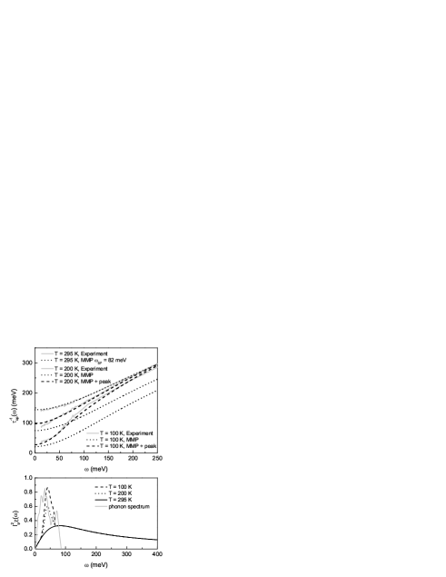
Figure 5: Top frame: optical scattering rates for Bi2212 at $T=295\,$K, $T=200\,$K, and $T=100\,$K. All are in the normal state. The gray solid lines are experiment of Tu et al.tu , dotted are theory based on an MMP-form for the charge carrier-exchange boson spectral density, and the dashed have in addition coupling to an optical resonance at $43\,$meV. The bottom frame shows the derived spectral density based on our well defined procedure to invert optical data. The $T=295\,$K spectrum has no resonance and is a pure MMP-form with $\omega_{sf}=82\,$meV (solid line). The other two spectra are modified through the addition of coupling to a resonance mode at $43\,$meV. Also shown is the phonon spectrum (gray solid curve).renker

temperatures, namely $T=100\,$K, $T=200\,$K, and $T=295\,$K. The data on the optical scattering rate was obtained by Tu et al.tu from their infrared measurements in Bi2212 and is denoted by gray solid lines (top to bottom is decreasing temperature). The black dotted lines are theory obtained from an MMP-form given by Eq. (13) with $\omega_{sf}=82\,$meV. The $T=295\,$K curve repeats the fit shown in the bottom frame of Fig. 4. The same spectral density, however, does not fit well the $T=200\,$K and $T=100\,$K data (dotted lines). To get agreement with these data sets it is necessary to augment the MMP-form by adding coupling to an additional optical resonance at $43\,$meV (this gives the dashed curves). This is the frequency at which inelastic neutron scattering experiments have revealed a strong peak in the magnetic susceptibility at momentum $(\pi,\pi)$ in the two dimensional Brillouin zone of the CuO₂ plane,fong in the superconducting state. The first report of such a resonance in neutron scattering was by J. Rossat-Mignot et al. for YBa₂Cu₃O_6+δ.ros We have already described our method for obtaining $I^{2}_{tr}\chi(\omega)$,mars4 ; mars5 ; schach4 ; schach7 ; schach5 ; schach8 ; schach9 thus it is not necessary to give details here except to mention that Tu et al.tu also get this peak using a slightly different method. We present final results for our model $I_{tr}^{2}\chi(\omega)$ in the bottom frame of Fig. 5. While no peak at $43\,$meV is observed at $T=295\,$K (solid line) one shows up at lower temperatures, dotted line for $T=200\,$K and a somewhat bigger peak at $T=100\,$K (dashed curve). At present, neutron scattering does not reveal a spin resonance at these temperatures. Returning to the top frame of Fig. 5 we stress that the introduction of a resonance peak in addition to the MMP-form is responsible for the observed rapid rise around $50\,$meV in the optical scattering rate at $T=100\,$K and also, although less obvious, at $T=200\,$K. The model spectral density fits the data remarkably well. Such optical resonances have been seen before in YBa₂Cu₃O_6.96schach4 as well as in Tl compoundsschach5 ; schach9 in the superconducting state of optimally doped samples, and have their equivalent in spin resonances observed by inelastic neutron scattering.fong ; ros ; dai ; he Here the high temperature optical resonances in Bi2212 are seen for the first time in the normal state above $T_{c}$, as reported by Tu et al.tu Their exact microscopic origin, however, cannot be deduced from optical data alone. It could be that the $43\,$meV neutron spin resonance forms above $T_{c}$ in this optimally doped material. Alternatively one might argue that this may be a phonon contribution (see gray solid curve in the bottom frame of Fig. 5) to the total electron-boson transport spectral density. If this were the case, however, we would not expect the peak of Fig. 5 (bottom frame) to show significant temperature dependence in this temperature regime. Also, the phonon peak in the bottom frame of Fig. 5 has more weight at low $\omega$ than is indicated in optics. In terms of the area under the spectral density $I^{2}_{tr}\chi(\omega)$ we note that the peak itself contributes less than about 15% of the total weight (at $T=100\,$K), the rest comes from the MMP-form. While the issue of the origin of the peak is important, here we concentrate instead on the consequences of its existence for the ARPES data. The possibility of coupling to a resonance mode has been discussed in the past in connection with such data.norm1 ; norm2 ; norm3

In Fig. 6 we compare our theoretical results for the

Figure 6: Top frame: the renormalized quasiparticle dispersion $E_{\bf k}$ as a function of the bare band energy $\varepsilon_{\bf k}$ in meV (light dash-dotted). The solid curve is based on the spin fluctuation spectral density with resonance peak obtained from conductivity data (Fig. 5) scaled down to a mass renormalization of $\lambda=1.28$, otherwise left unmodified. The heavy dash-dotted curve is for comparison and has no resonance peak. The light dashed straight line is for comparison and is the ARPES “bare dispersion” obtained by making the curve go through experiment at $253\,$meV. This corresponds to a theoretical $\varepsilon_{\bf k}=327\,$meV at $k-k_{F}=0.089\,$Å^-1, much greater than the ARPES ‘bare’ value. This frame applies to $T=130\,$K and is in the normal state. The bottom frame is for $T=70\,$K in the superconducting state.

renormalized quasiparticle energies with the ARPES experimental data (solid squares). The theory (solid curve) is based on the optics derived spectral density (see Fig. 5, bottom frame). The top frame is for $T=130\,$K in the normal state and the bottom frame is for $T=70\,$K in the superconducting state. For the top frame we renormalized downward the $I^{2}_{tr}\chi(\omega)$ to account for the expectation that in a spin fluctuation mechanism the quasiparticle electron-boson interaction spectral density should be smaller than its transport counterpart. To get the fit seen in the figure we used $\lambda=1.28$. A smaller value of $\lambda=1.09$ was used in the bottom frame. We see that we can get an equally good fit to ARPES with spin fluctuations including the $43\,$meV resonance as we did with phonons. This new fit (see Fig. 6), however, has the advantage that it can equally well explain the optical data while this is impossible with phonons. It is also clear from the calculations that the transport electron-boson interaction spectral density is larger than the quasiparticle spectral density by a factor of about two as is expected in theories of the NAFFL model. It should be acknowledged, however, that part of the difference in the value of $\lambda$ needed to fit ARPES data as compared with optics reflects anisotropies in the quasiparticle renormalizations over the Brillouin zone.

Also included in the two frames of Fig. 6 are our results for a $E_{\bf k}$ (heavy dash-dotted) when the resonant peak in the spectral density is left out of the calculations. We see that the pronounced structure at $k-k_{F}\sim 0.04\,$Å^-1 seen in the superconducting state is not reproduced in this case. If we used instead the MFL model, i.e.: $I^{2}\chi(\omega)=I^{2}\theta(\omega_{max}-\omega)$, the deviation from the data would be worse and even clearly seen in the normal state. The resonance peak, absent in the MMP-form and in the MFL model, is what gives the observed structure. Also shown in the figure is the the bare dispersion relation (light dash-dotted curve) on which our calculations are based. This is quite different from the ARPES derived ‘bare’ dispersion, the light dashed curve, obtained by making the curve go through the experimental point at $253\,$meV on the assumption that the renormalization by boson-exchange interaction has ended at this energy. Reference to the difference between the theoretical bare dispersion (light dash-dotted) and the dressed curve (solid line) shows clearly that this is not the case in a spin fluctuation model.

It is interesting to note the similarities and differences between our work and that of Verga et al.verga An important difference is that these authors invert the ARPES data directly from which they obtain a model electron-boson spectral density. Instead, we have inverted the optical data which serves as a second constraint on the microscopics not considered by Verga et al. While they invert data in LSCO at three different doping levels $x$, they, nevertheless, find a spectrum which has a peak which is, however, not as prominent as either the spin resonance peak or the phonon peak in the bottom frame of our Fig. 5. Their peak could simply be a peak of the MMP-form as in the solid black curve in the bottom frame of Fig. 5. Nothing definite can be concluded. However, we point out that they do find tails at higher energies ($\omega>100\,$meV), as we have, which rather support spin fluctuations and not phonons. In this paper we consider in addition to ARPES optical data and from this we conclude more forcefully that high energy tails extending up to several hundred meV exist in the boson assisted spectral functions describing the electron boson interaction in Bi2212.

Whatever the mechanism by which the quasiparticles are renormalized the $(11)$-component of the $2\times 2$ Nambu Green’s function in the superconducting state can be expressed in the general formmars6

$$G_{11}({\bf k},\omega)=\frac{\omega Z_{\bf k}(\omega)+\varepsilon_{\bf k}}{\omega^{2}Z^{2}_{\bf k}(\omega)-\varepsilon^{2}_{\bf k}-\tilde{\Delta}^{2}_{\bf k}(\omega)},$$ (15)

where the renormalized frequency $\tilde{\omega}(\omega)\equiv\omega Z(\omega)$. The inverse quasiparticle lifetime is defined as twice the imaginary part of the poles of $G_{11}({\bf k},\omega)$ for a given momentum label k. For $\omega=E_{\bf k}-i\Gamma_{\bf k}$ we obtainmars6

$$\Gamma_{\bf k}=\frac{E_{\bf k}Z_{{\bf k}2}(E_{\bf k})}{Z_{{\bf k}1}(E_{\bf k})}-\frac{\tilde{\Delta}_{{\bf k}1}(E_{\bf k})\tilde{\Delta}_{{\bf k}2}(E_{\bf k})}{E_{\bf k}Z^{2}_{{\bf k}1}(E_{\bf k})},$$ (16)

where the indices 1 and 2 refer to the real and imaginary part respectively, and the corresponding renormalized energy is a solution of

$$E_{\bf k}=\sqrt{\frac{\varepsilon^{2}_{\bf k}+\tilde{\Delta}^{2}_{{\bf k}1}(E_{\bf k})}{Z^{2}_{{\bf k}1}(E_{\bf k})}}.$$ (17)

For the normal state $(\tilde{\Delta}_{\bf k}(\omega)=0)$ these expressions reduce to those previously given in the limit of weak scattering with the modification that $\Gamma$ is renormalized by a mass enhancement factor $(1+\lambda)$.

In Fig. 7 we emphasize once again the difference obtained

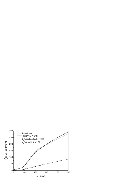
Figure 7: Comparison between scattering rates as a function of frequency $\omega$ obtained from optics and from ARPES. The gray solid line is the experimental optical scattering rate at $T=80\,$K obtained from the work of Tu et al.tu while the black solid curve is our theoretical result based on the electron-spin fluctuation spectral density $I^{2}_{tr}\chi(\omega)$ shown in the bottom frame of Fig. 5 (but using data for $T=80\,$K). The other two curves are theoretical results for the imaginary part of the quasiparticle self energy.

between quasiparticle scattering rates and its optical counterpart. It applies to $T=80\,$K for Bi2212 in the superconducting state. The gray solid curve represents the data of Tu et al.tu for the optical scattering rate and the solid line our theoretical fit to this data which also determines the transport spectral density $I^{2}_{tr}\chi(\omega)$. The corresponding value of $\lambda_{tr}$ is 2.18. Consideration of the ARPES data on quasiparticle renormalizations shows us that the equilibrium spectral density $I^{2}\chi(\omega)$ must be considerably smaller. To calculate the imaginary part of $\Gamma(\omega)$ of Eq. (16) we have reduced $I^{2}_{tr}\chi(\omega)$ by a factor of two but without changing its shape. This is done to get reasonable agreement with ARPES shown in Fig. 6. The results are shown as dashed and dotted lines for the antinodal and nodal directions respectively. Not only is the shape of the resulting scattering rate different from the frequency variation obtained in the optical case but its magnitude is also different reflecting the difference in magnitude of $I^{2}_{tr}\chi(\omega)$ and $I^{2}\chi(\omega)$.

V Conclusion

We have reconsidered the interpretation of the quasiparticle renormalizations observed in high resolution ARPES data for the specific case of Bi2212. We confirm that the observed energy scale is compatible with coupling to phonons. We find, however, that present data and, in particular, the way they are analyzed might well significantly underestimate renormalization due to other boson exchange mechanisms distinct from phonon exchange and for which the energy scale is larger. As an example this would be the case in a spin fluctuation exchange mechanism as is envisaged in the NAFFL model where the energy scale for the spin fluctuations is set by $J$ of the $t-J$ model and is consequently very high.

If in addition to ARPES, optical data is also considered, it is found that an explanation in terms of phonons becomes less tenable. Of course, there are many complications and these make a definitive interpretation impossible. What is clear, however, is that transport properties and in particular the observed infrared conductivity cannot be understood as due to the electron-phonon interaction. This holds even if modifications are introduced to account for the reduced screening present in the cuprates because of the low electron density and also the increased effects of correlations. The main point is that the underlying charge carrier-phonon spectral density is cut off at the maximum phonon frequency and this feature is in conflict with optical data. By contrast, spin fluctuations give a natural explanation of the data. Our analysis of the data of Tu et al.tu also provides a natural explanation of the ARPES data. What we find is that an optical resonance is present in the infrared data even in the normal state above $T_{c}$ and this resonance can explain the energy scale seen in ARPES. (Below $T_{c}$ this optical resonance has a spin resonance equivalent observed by Fong et al.fong using inelastic neutron scattering.) The microscopic nature of the optical resonance is not entirely known. It could have its origin in spin fluctuations theories and be the spin one resonance observed in inelastic polarized neutron scattering experiments, or could even contain a phonon contribution over and beyond the spin fluctuation contribution.

Our analysis of both ARPES and optical data together has served to emphasize once more the differences between the equilibrium electron-boson exchange spectral density $\alpha^{2}F(\omega)$ and its transport counterpart $\alpha^{2}_{tr}F(\omega)$ be it for phonon exchange or spin fluctuations. The data indicates that these two quantities differ in magnitude by roughly a factor of two or so. This is understood to arise from the fact that transport scattering rates emphasize more strongly backward collisions than do equilibrium rates. While detailed and elaborate calculations beyond the scope of this paper would be required to pin down the expected differences quantitatively, present ideas about reduced screening in the cuprates lead directly to the expectation that phonons will be much less important in transport than for equilibrium properties while ideas about the NAFFL model lead to opposite expectations. Spin fluctuations dominate the transport while at the same time could be less important in determining quasiparticle properties. This agrees well with the available combined set of optical and ARPES data in Bi2212.

- (1) A. Kaminski, J. Mesot, H. Fretwell, J.C. Campuzano, M.R. Norman, M. Randeria, H. Ding, T. Sato, T. Takahashi, T. Mochiku, K. Kadowaki, and H. Hoechst, Phys. Rev. Lett. 84, 1788 (2000).
- (2) T. Valla, A.V. Fedorov, P.D. Johnson, J. Xue, K.E. Smith, and F.J. DiSalvo, Phys. Rev. Lett. 85, 4759 (2000).
- (3) P.D. Johnson, T. Valla, A.V. Fedorov, Z. Yusof, B.O. Wells, Q. Li, A.R. Moodenbaugh, G.D. Gu, N. Koshizuka, C. Kendziora, Sha Jian, and D.G. Hinks, Phys. Rev. Lett. 87, 177007 (2001).
- (4) A. Kaminski, M. Randeria, J.C. Campuzano, M.R. Norman, H. Fretwell, J. Mesot, T. Sato, T. Takahashi, and K. Kadowaki, Phys. Rev. Lett. 86, 1070 (2001).
- (5) A. Lanzara, P.V. Bogdanov, X.J. Zhou, S.A. Kellar, D.L. Feng, E.D. Lu, T. Yoshida, H. Eisaki, A. Fujimori, K. Kishio, J.-I. Shimoyama, T. Noda, S. Uchida, Z. Hussain, and Z.-X. Shen, Nature (London) 412, 510 (2001).
- (6) P.V. Bogdanov, A. Lanzara, S.A. Kellar, X.J. Zhou, E.D. Lu, W.J. Zheng, G. Gu, J.-I. Shimoyama, K. Kishio, H. Ikeda, R. Yoshizaki, Z. Hussain, and Z.-X. Shen, Phys. Rev. Lett. 85, 2581 (2000).
- (7) T. Valla, A.V. Fedorov, P.D. Johnson, B.O. Wells, S.L. Hulbert, Q. Li, G.D. Gu, N. Koshizuka, Science 285, 2110 (1999).
- (8) T. Valla, A.V. Fedorov, P.D. Johnson, Q. Li, G.D. Gu, and N. Koshizuka, Phys. Rev. Lett. 85, 828 (2000).
- (9) F. Marsiglio and J.P. Carbotte, in Handbook on Superconductivity: Conventional and Unconventional, eds. K.H. Bennemann and J.B. Ketterson (Springer, Berlin, in print).
- (10) W.N. Hardy, D.A. Bonn, D.C. Morgan, R. Liang, and K. Zhang, Phys. Rev. Lett. 70, 3999 (1993).
- (11) Z.-X. Shen, D.S. Dessau, B.O. Wells, D.M. King, W.E. Spicer, A.J. Arko, D. Marshall, L.W. Lombardo, A. Kapitulnik, P. Dickinson, S. Doniach, J. DiCarlo, A.G. Loeser, and C.H. Park, Phys. Rev. Lett. 70, 1553 (1993).
- (12) D.H. Wollman, D.A. Van Harlingen, W.C. Lee, D.M. Ginsberg, and A.J. Leggett, Phys. Rev. Lett. 71, 2134 (1993).
- (13) C.C. Tsuei, J.R. Kirtley, C.C. Chi, LockSeeYu-Jahnes, A. Gubta, T. Shaw, J.Z. Sun, and M.B. Ketchen, Phys. Rev. Lett. 73, 593 (1994).
- (14) P. Tomlinson and J.P. Carbotte, Phys. Rev. B13, 4738 (1976).
- (15) J.P. Carbotte, in Anisotropy Effects in Superconductors, ed. H.W. Weber, Plenum (New York, 1977), p. 183.
- (16) M.L. Kulić, Phys. Rep. 338, 1 (2000).
- (17) R. Zeyher and M.L. Kulić, Phys. Rev. B53, 2850 (1996); 54, 8985 (1996).
- (18) M.L. Kulić and R. Zeyher, Phys. Rev. B49, 4395 (1994); Physica C 199-200, 358 (1994); 235-240, 358 (1994).
- (19) M. Weger, B. Barbelini, and M. Peter, Z. Phys. B 94, 387 (1994).
- (20) M. Weger, M. Peter, and L.P. Pitaevskii, Z. Phys. B 101, 573 (1996).
- (21) O.V. Danylenko, O.V. Dolgov, M.L. Kulić, and V. Oudovenko, Euro. Phys. Jour. B-Cond. Matter 9, 201 (1999).
- (22) M.L. Kulić and O.V. Dolgov, in High Temperature Superconductivity, ed.: S. Barnes, J. Ashkenazi, J. Cohn, and F. Zuo, AIP Conference Proceedings 483, 63 (1999).
- (23) S. Sorella, G.B. Martins, F. Becca, C. Gazza, L. Capriotti, A. Parola, and E. Dagotto, Phys. Rev. Lett. 88, 117002 (2002).
- (24) A.J. Millis, H. Monien, and D. Pines, Phys. Rev. B42, 167 (1990).
- (25) P. Monthoux and D. Pines, Phys. Rev. B47, 6069 (1993); Phys. Rev. B49, 4261 (1994); Phys. Rev. B50, 16015 (1994).
- (26) C.M. Varma, Int. J. Mod. Phys. 3, 2083 (1989).
- (27) P.B. Littlewood, C.M. Varma, S. Schmitt-Rink, and E. Abrahams, Phys. Rev. B39, 12371 (1989).
- (28) C.M. Varma, P.B. Littlewood, S. Schmitt-Rink, E. Abrahams, and A.E. Ruckenstein, Phys. Rev. Lett. 63, 1996 (1989); ibid. 64, 497 (1990).
- (29) A.V. Puchkov, D.N. Basov, and T. Timusk, J. Phys.: Condens. Matter 8, 10049 (1996).
- (30) T. Timusk and B. Statt, Rep. Prog. Phys. 62, 61 (1999).
- (31) J.J. Tu, C.C. Homes, G.D. Gu, D.N. Basov, and M. Strongin, Phys. Rev. B66, 144514 (2002).
- (32) P. Tomlinson and J.P. Carbotte, Can. J. Phys. 55, 751 (1977).
- (33) H.K. Leung, F.W. Kus, N. McKay, and J.P. Carbotte, Phys. Rev. B16, 4358 (1977).
- (34) P.B. Allen, Phys. Rev. B3 305 (1971).
- (35) G. Grimvall, The Electron-Phonon Interaction in Metals, (North-Holland, New York, 1981).
- (36) J.P. Carbotte, Rev. Mod. Phys. 62, 1027 (1990).
- (37) J.M. Daams and J.P. Carbotte, J. Low Temp. Phys. 43, 263 (1981).
- (38) W.L. McMillan and J.M. Rowell, Phys. Rev. Lett. 19, 108 (1965).
- (39) W.L. McMillan and J.M. Rowell, in Superconductivity, ed. R.D. Parks (Marcel Dekker Inc., New York, 1969), p. 561.
- (40) A. Virosztek and J. Ruvalds, Phys. Rev. B42, 4064 (1990).
- (41) J. Ruvalds and A. Virosztek, Phys. Rev. B43, 5498 (1991).
- (42) S.Y. Savrasov and O.K. Andersen, Phys. Rev. Lett. 77, 4430 (1996).
- (43) D. Branch and J.P. Carbotte, Phys. Rev. B52, 603 (1995); J. Supercond. 12, 667 (1999); Can. J. Phys. 77, 531 (1999); J. Supercond. 13, 535 (2000).
- (44) J.P. Carbotte, E. Schachinger, and D.N. Basov, Nature (London) 401, 354 (1999).
- (45) F. Marsiglio, T. Startseva, and J.P. Carbotte, Phys. Lett. A 245, 172 (1998).
- (46) E. Schachinger, J.P. Carbotte, and D.N. Basov, Europhys. Lett. 54, 380 (2001).
- (47) E. Schachinger and J.P. Carbotte, Phys. Rev. B62, 9054 (2000).
- (48) E. Schachinger and J.P. Carbotte, Phys. Rev. B64, 094501 (2001).
- (49) S. Verga, A. Knigavko, and F. Marsiglio, cond-mat/0207145 (unpublished).
- (50) B. Renker, F. Gompf, D. Ewert, P. Adelmann, H. Schmidt, E. Gering, and H. Mutka, Z. Phys. B 77, 65 (1989).
- (51) F. Marsiglio and J.P. Carbotte, Aust. J. Phys. 50, 975 (1997); Aust. J. Phys. 50, 1011 (1997).
- (52) H.F. Fong, P. Bourges, Y. Sidis, L.P. Regnault, A. Ivanov, G.D. Gull, N. Koshizuka, and B. Keimer, Nature (London) 389, 588 (1999).
- (53) J. Rossat-Mignot, L.P. Regnault, C. Vettier, P. Bourges, P. Burlet, J. Bossy, J.Y. Henry, and G. Lapertot, Physica C 185-189, 86 (1991).
- (54) F. Marsiglio, Molecular Physics Reports 24, 73 (1999).
- (55) E. Schachinger and J.P. Carbotte, Physica C 364, 13 (2001).
- (56) P. Dai, H.A. Mook, S.M. Hayden, G. Aeppli, T.G. Perring, R.D. Hunt, and F. Doğan, Science 284, 1344 (1999).
- (57) H. He, P. Bourges, Y. Sidis, C. Ulrich, L.P. Regnault, S. Pailhès, N.S. Berzigiarova, N.N. Kolesnikov, and B. Keimer, Science 295, 1045 (2002).
- (58) M.R. Norman and H. Ding, Phys. Rev. B57, R11 089 (1998).
- (59) M.R. Norman, M. Eschrig, A. Kaminski, and J.C. Campuzano, Phys. Rev. B64, 184508 (2001).
- (60) M. Eschrig and M.R. Norman, Phys. Rev. B67, 144503 (2003).