Reduction of the sign problem using the meron-cluster approach.

Abstract

The sign problem in quantum Monte Carlo calculations is analyzed using the meron-cluster solution. The concept of merons can be used to solve the sign problem for a limited class of models. Here we show that the method can be used to reduce the sign problem in a wider class of models. We investigate how the meron solution evolves between a point in parameter space where it eliminates the sign problem and a point where it does not affect the sign problem at all. In this intermediate regime the merons can be used to reduce the sign problem. The average sign still decreases exponentially with system size and inverse temperature but with a different prefactor. The sign exhibits the slowest decrease in the vicinity of points where the meron-cluster solution eliminates the sign problem. We have used stochastic series expansion quantum Monte Carlo combined with the concept of directed loops.

I Introduction

To stochastically study a quantum problem using a quantum Monte Carlo method it is necessary to transform it to a form that is similar to a classical statistical problem. The sign problem appears when this transformation leads to a weight function that is not positive definite. As quantum Monte Carlo methods have become increasingly efficientEvertz et al. (1993); Kawashima et al. (1994); Prokof’ev et al. (1996); Beard and Wiese (1996); Sandvik (1999); Syljuåsen and Sandvik (2002) there is a notable lack of progress in solving the sign problem. The sign problem severely limits the number of models that can be studied using quantum Monte Carlo methods, and in particular there are only very few models of interacting fermions in higher dimensions that are accessible to existing algorithms.Blankenbecler et al. (1981)

The recent development of the so-called meron-cluster solutionChandrasekharan and Wiese (1999) has extended the range of models where the sign problem can be avoided. This method uses the properties of loop quantum Monte Carlo algorithms to establish a one-to-one mapping between configurations with negative weight and corresponding configurations with positive weight. These contributions cancel each other and a fraction of the phase space with a positive definite weight function is left, which can be sampled with no sign problem.

Unfortunately the meron solution works for only a rather limited class of models.Chandrasekharan et al. The main purpose of the present paper is to show that the meron concept can be applied also to models where the sign problem is not eliminated. We demonstrate that in a wider class of models it is possible to cancel out part of the negative configurations, and thereby reduce the sign problem. We investigate a model in an intermediate regime between a point in parameter space where the sign problem can be solved completely and a point where the meron-cluster algorithm cannot be applied. Our results show that the meron-cluster algorithm does indeed reduce the sign problem in this intermediate regime. The main focus of the study is frustrated spin models, but we also apply this method to spinless fermions.

The outline of the paper is as follows. In Sec. II the Monte Carlo algorithm is briefly explained. The sign problem and the meron-cluster algorithm are introduced in Sec. III. In Sec. IV a modified version of the stochastic series expansion is described. The origin of the sign problem for frustrated spin systems and fermions is discussed in Sec. V. In Sec. VI we demonstrate how the meron solution affects the average sign for a range of models where the sign problem cannot be eliminated. We conclude with summary and discussions in Sec. VII.

II The quantum Monte Carlo algorithm

In order to explain the meron-cluster solution introduced in Sec. IV we here give a summary of the stochastic series expansion (SSE) methodSandvik and Kurkijärvi (1991); Sandvik (1999); Syljuåsen and Sandvik (2002).

Consider a lattice model described by a Hamiltonian $H$. In the SSE method the partition function $Z$ is Taylor expanded,

$$Z=\sum_{\alpha}\sum_{m=0}^{\infty}\frac{\beta^{m}}{m!}\langle\alpha|(-H)^{m}|\alpha\rangle,$$ (1)

where $|\alpha\rangle$ are states in which the above matrix elements can be calculated and $\beta$ denotes the inverse temperature.

For sake of clarity we will now consider a one-dimensional ferromagnetic Heisenberg model,

$$H=-\sum_{i=1}^{N}S_{i}^{z}S_{i+1}^{z}+\frac{1}{2}\left(S_{i}^{+}S_{i+1}^{-}+S_{i}^{-}S_{i+1}^{+}\right),$$ (2)

where $N$ denotes th number of sites. The Hamiltonian is rewritten as a sum over diagonal and off-diagonal operators,

$$-H=\sum_{i=1}^{N}(H_{1,i}+H_{2,i}),$$ (3)

where

$$H_{1,i}=S_{i}^{z}S_{i+1}^{z}+C$$ (4)

and

$$H_{2,i}=\frac{1}{2}(S_{i}^{+}S_{i+1}^{-}+S_{i}^{-}S_{i+1}^{+}),$$ (5)

where $C$ is a constant inserted to assure that the expectation value $\langle\alpha|H_{1,i}|\alpha\rangle$ is positive for all states $|\alpha\rangle$.

To simplify the Monte Carlo update we introduce an additional unit operator $H_{0,0}=1$. Inserting the Hamiltonian given by Eq. (3) into Eq. (1), and truncating the sum at $m=L$ we obtain

$$Z=\sum_{\alpha}\sum_{S_{L}}\frac{\beta^{n}(L-n)!}{L!}\langle\alpha|\prod_{k=1}^{L}H_{a_{k},i_{k}}|\alpha\rangle,$$ (6)

where $n$ stands for the number of non-unit operators, and $S_{L}$ denotes a sequence of operator-indices

$$S_{L}=(a_{1},i_{1}),(a_{2},i_{2}),...,(a_{L},i_{L}),$$ (7)

with $a_{k}={1,2}$ and $i_{k}={1,\ldots,N}$, or $(a_{k},i_{k})=(0,0)$.

The Monte Carlo procedure must sample the space of all states $|\alpha\rangle$, and all sequences $S_{L}$. The simulation starts with some random state $|\alpha\rangle$ and an operator string containing only unit operators. One Monte Carlo step consists of a diagonal and an off-diagonal update. In the diagonal update attempts are made to exchange unit and diagonal operators sequentially at each position in the operator string. The probability for inserting or deleting a diagonal operator in the operator string is given by detailed balance.Sandvik (1999)

The off-diagonal update, also called loop update, is carried out with $n$ fixed. Each bond operator $H_{i_{k}}=H_{1,i_{k}}+H_{2,i_{k}}$ acts only on two spins, $S_{i_{k}}$ and $S_{i_{k}+1}$. We can therefore rewrite the matrix elements in Eq. (6) as a product of $n$ terms, called vertices,

$$M(\alpha,S_{L})=\prod_{k=1}^{n}W_{k},$$ (8)

where the vertex weight $W_{p}$ is defined as

$$W_{p}=\langle S^{z}_{i_{p}}(p)S^{z}_{i_{p}+1}(p)|H_{i_{p}}|S^{z}_{i_{p}}(p-1),S^{z}_{i_{p}+1}(k-1)\rangle$$

(9)

where $S^{z}_{i}(p)$ denotes the state of spin $i$ in a propagated state, defined by

$$|\alpha(p)\rangle\sim\prod_{k=1}^{p}H_{a_{k},i_{k}}|\alpha\rangle.$$ (10)

A vertex thus consists of four spins, called the legs of the vertex, and an operator. Each term in the expansion in Eq. (6) can be viewed as a sequence of vertices. An example of one term for a four-site chain is shown in the left part of Fig. 1.

Figure 1: In the left part of the figure one of the terms in the expansion in Eq. (6) is shown. The two different states of the basis, spin up and down, are illustrated with circles and diamonds and the operators are depicted as horizontal bars. In the right part of the figure the configuration is divided up into closed loops. The two loops in the configuration are distinguished by different line styles.

The principles of the off-diagonal update are: one of the $n$ vertices is chosen at random and one of its four legs is randomly selected as the entrance leg. The spin of the entrance leg is flipped. One of the legs of the operator is chosen as the exit leg, and its state is also changed. The exit leg is chosen with a probability calculated from the weight of the obtained vertex.Sandvik (1999) Thereafter the vertex list is sequentially searched for the next vertex that includes the exit spin. This spin becomes the entrance leg of the next vertex and the procedure is continued until the original entrance leg is reached. During one Monte Carlo step the loop update is repeated until on average half of the vertices have been updated.

In the method described above the spin states are altered as the loop is constructed. During one Monte Carlo step a given spin can be part of several different loops, or it may be of none. In a few special cases, such as for the isotropic Heisenberg model, the propagation of each loop through the lattice is deterministic, meaning that there is only one possible exit leg for each entrance leg.Sandvik (1999) In these special cases it is possible to divide the whole space-time lattice up into loops so that each and every spin belongs to only one loop. An example of such a configuration is shown in the right part of Fig. 1. The loop update can then be modified to identifying the unique loop structure and flipping each loop with probability one half.

III The Sign Problem

In this section we show how the sign problem appears in quantum Monte Carlo simulations and introduce the recent meron approach to solving the sign problem. We start by considering a general form of an expectation value that can be calculated by Monte Carlo methods,

$$\langle A\rangle=\frac{\sum_{i}A(x_{i})W(x_{i})}{\sum_{i}W(x_{i})}=\langle A(x)\rangle_{W},$$ (11)

where the weight function $W(x_{i})$ and $A(x_{i})$ depend on the configuration $x_{i}$. When the coordinates $x_{i}$ are sampled according to relative weight, the expectation value is given by the average value of $A(x)$ as indicated in the last part of Eq. (11). The sign problem appears if the weight function is not positive. In this case the sampling can be done using the absolute value of the weight,

$$\langle A\rangle=\frac{\langle As\rangle_{|W|}}{\langle s\rangle_{|W|}},$$ (12)

where $s$ denotes the sign of the weight function and equals $\pm 1$. However, in many cases of physical interest the average sign approaches zero exponentially as the system size is increased. The above expectation value will then suffer from very large statistical fluctuations since it becomes a ratio of two small numbers. Let us now consider how negative weight functions appear for quantum mechanical systems. The weight function $W(\alpha,S_{L})$ corresponding to the partition function given by Eq. (6) is

$$W(\alpha,S_{L})=\frac{\beta^{n}(L-n)!}{L!}\langle\alpha|\prod_{k=1}^{L}H_{a_{k},i_{k}}|\alpha\rangle,$$ (13)

This is strictly positive, and for the ferromagnet there is no sign problem. Let us next consider an antiferromagnet. In this case the diagonal and off-diagonal operators are of the form

$$H_{1,b}=-S_{i(b)}^{z}S_{j(b)}^{z}+C,$$ (14)

and

$$H_{2,b}=-\frac{1}{2}(S_{i(b)}^{+}S_{j(b)}^{-}+S_{i(b)}^{-}S_{j(b)}^{+}).$$ (15)

By adjusting the constant $C$ it is still possible to have $\langle\alpha|H_{1,b}|\alpha\rangle\geq 0$. However, for the off-diagonal operator the expectation value $\langle\alpha|H_{2,b}|\alpha\rangle\leq 0$, and the sign must be taken into account. If there is an odd number of off-diagonal operators in the configuration the sign of the weight function will be negative. Due to the periodic boundary conditions in the imaginary time direction the number of off-diagonal operators on a square lattice is always even and there is no sign problem. However, if the system is frustrated, as on a triangular lattice, the sign problem appears for the antiferromagnetic spin model. For a fermionic system the anticommutator rules must be taken into account and the sign of the configuration changes sign every time two fermion world lines wrap around each other in imaginary time. We therefore see that both for frustrated spin models and fermionic models the sign problem enters into the loop update. Flipping a loop can cause the number of spin flipping operators to change parity, or it can cause two fermions to permute and thereby change the sign. Loops that cause the sign to change are called merons,Chandrasekharan and Wiese (1999) and in some cases one can, in effect, solve the sign problem by avoiding configurations that include merons.

In order to explain the meron solution we need to revisit the loop update. As was pointed out at the end of the previous section it is sometimes possible to divide the lattice up into a unique loop structure. Expectation values can then be calculated using so-called improved estimators, which are averages over all possible loop configurations. If the number of loops in the system is given by $N_{L}$ there are $2^{N_{L}}$ configurations that can be reached by flipping the loops, since all the loops can be in two states. The expectation value in Eq. (12) can therefore be rewritten as

$$\langle A\rangle=\frac{\langle\langle A(x)s(x)\rangle\rangle_{|W|}}{\langle\langle s(x)\rangle\rangle_{|W|}},$$ (16)

where the double expectation brackets denote an average over the different loop configurations

$$\langle\langle s(x)A(x)\rangle\rangle_{|W|}=\langle\frac{1}{2^{N_{L}}}\sum_{l=1}^{2^{N_{L}}}s(x_{l})A(x_{l})\rangle_{|W|}.$$ (17)

If certain criteria are fulfilled, the expectation value can be expressed as

$$\langle A\rangle=\langle\langle A(x)\delta_{n_{M},0}\rangle\rangle_{|W|},$$ (18)

where $n_{M}$ is the number of merons. Therefore only configurations without sign changing loops give non-zero contributions to the expectation value, and the sign problem is, in effect, solved.

Let us examine the necessary conditions for this to be the case:

1. The lattice can be divided up into loops so that each spin belongs to one and only one loop.

2. The weight must not change when the loops are flipped.

3. The loops must affect the sign independently.

4. The zero-meron sector must be positive definite.

5. The expectation value of the operator is unchanged when a loop is flipped.

Together these conditions place severe restrictions on which models can be studied with the meron solution. Our aim is to examine if the conditions can be relaxed to allow for a more general algorithm. Of the five conditions the last one is the least severe. Many operators for which this condition does not hold can be expressed by introducing the two-meron sector.Chandrasekharan and Wiese (1999); Henelius and Sandvik (2000) Examples of operators for which the last condition holds are the energy and heat capacity, which in SSE are given by

$$E = -\frac{\langle n\rangle}{\beta}$$ (19)

$$C = \langle n^{2}\rangle-\langle n\rangle^{2}-\langle n\rangle.$$ (20)

where $n$ is the number of non-unit operators in the operator string.

The first three conditions are severe and we are not aware of a way to relax these restrictions. In this study we examine the case when the fourth condition is not met, and the zero-meron sector is not positive definite. If this is not the case Eq. (18) must be replaced by

$$\langle A\rangle=\frac{\langle\langle A(x)s(x)\delta_{n_{M},0}\rangle\rangle_{|W|}}{\langle\langle s(x)\delta_{n_{M},0}\rangle\rangle_{|W|}},$$ (21)

where $s(x)$ is the sign of the configuration in the zero meron sector. The higher meron sectors do not contribute to the average and the sign problem is therefore reduced, but not eliminated. To find out how the average sign changes by leaving out the non-zero meron sectors is the aim of this investigation. It is not clear whether the exponential character of the sign problem will change, or how the system size will affect the average sign. This depends on the relative weight of the different meron sectors and on the average sign in the zero-meron sector.

In order to investigate systems where condition four does not hold it is necessary to satisfy the first three criteria. As was stated at the end of Sec. II there are a few special cases where a unique loop structure exists, and in these cases the first condition is automatically satisfied. For more general models, where one can choose between different exit legs, this is not true, since there no longer exists a unique way to divide the lattice into loops. It is, however, possible to cover the lattice with loops so that each spin belongs to one and only one loop. This can be done by always choosing an exit leg that is not already part of any loop. Since a unique loop structure does not exist one also has to sample all possible loop configurations, and in order to implement the meron solution efficiently this has to be done without leaving the zero and two-meron sectors. We have implemented a loop update that inherently divides the lattice up in separate loops. This can be done as long as the bounce process, where the entrance and exit legs coincide, can be neglected. With the advent of directed loopsSyljuåsen and Sandvik (2002) there now exists a way to eliminate the bounce process in many models of interest. In the next section we will introduce the idea of directed loops and intoroduce models where the first three, but not the forth, conditions are satisfied.

IV SSE Loop Construction

Following Ref. Syljuåsen and Sandvik, 2002 we here derive the directed loops equations that enable us to neglect the bounce process, and explicitly show that the weight in the extended space of directed loops is unaltered when a loop is flipped. Then we will describe a modification to the SSE loop update and demonstrate how the meron approach can be efficiently implemented also for models where there is not a unique way of dividing the lattice into loops.

By considering that each possible loop has a “time-reversed” counterpart it was shownSyljuåsen and Sandvik (2002) that a loop move satisfies detailed balance if, for every vertex that the loop passes through,

$$W_{s}P(s,i\rightarrow j)=W_{s^{\prime}}P(s^{\prime},j\rightarrow i),$$ (22)

where the vertex weight $W_{s}$ for a given spin configuration $s$ is defined by Eq. (9) and $P(s,i\rightarrow j)$ is the probability to choose exit leg $j$ given entrance leg $i$ for a given spin configuration $s$.

The main idea of the method of directed loops is to attach weight also to the link that connects the entrance and exit spins at a traversed vertex. The weight of a vertex in this extended space can then be written as $W(s,i,j)$. We are allowed to introduce such auxiliary variables if the sum over auxiliary variables reduces to the original weight

$$\sum_{j}W(s,i,j)=W_{s}.$$ (23)

We furthermore require that the weight in this extended space is not affected by flipping a loop, which translates to

$$W(s,i,j)=W(s^{\prime},j,i).$$ (24)

Considering the criteria for detailed balance, Eq. (22) we can now relate the weights in the original and extended space as

$$W(s,e,x)=W_{s}P(s,e,x).$$ (25)

We have therefore shown that the total weight in our extended configuration space is unchanged when flipping a loop, and the second condition for using the meron solution is therefore fulfilled. The method of directed loops is a way to assign probabilities to the different possible exit legs given an entrance leg. The probabilities are determined by solving the system of equations that Eq. (22) and Eq. (24) generate. We want to emphasis that for many models it is possible to solve the equations so that the bounce process is forbiddenSyljuåsen and Sandvik (2002), and as we now show this makes it possible to divide the lattice up into separate loops.

Next we describe a new procedure that enables us to make this division. In our new update the physical structure of the loops is determined and updated during the diagonal move, while each loop is flipped with probability one half in the off-diagonal update. The diagonal move is quite different from the one described in section II and we here describe it in some detail.

The operator string is, as before, updated sequentially, and if a unit operator is encountered an attempt to insert a diagonal operator is made. If an operator is inserted its four legs are linked to the existing loops. If the bounce is eliminated there are three possible ways to link the entrance and exit legs of a vertex, see Fig. 2. The decision of which configuration to use is based on detailed balance equations, which states that the probability of different vertices is proportional to their weight given by Eq. 9. It is enough to treat an arbitrary leg as “entrance leg” to the vertex and determine an exit leg. With two legs connected together in this manner the other two legs are also automatically linked. If instead a diagonal operator is encountered, an attempt is made to exchange it for a unit operator, as in the standard diagonal update. If the removal is not accepted an attempt is made to alter the way in which the legs are connected. In the same way as when inserting a new diagonal operator an “exit leg” is determined for an arbitrary “entrance leg”, a procedure which may change the existing links . This change of loop structure is also done if an off-diagonal operator is encountered. We graphically demonstrate this modified update in Fig. 3. On the left side of Fig. 3 a term in the SSE expansion is divided up into loops. A possible outcome after a diagonal update is shown on the right. In the next section we will apply this update to models that suffer from the sign problem.

Figure 2: The three different ways the legs of a vertex can be paired together, if the bounce process is neglected, are marked by letters A,B and C. The fourth vertex shows one example of the many possible ways to connect the legs if the bounce is allowed.

Figure 3: A example of a SSE configuration divided up into separate loops is depicted on the left side. In the right part of the figure a possible outcome after a sequential diagonal update is shown. One operator has been inserted and the way the legs are connected has been changed for two of the vertices. These operators are marked with a thick bar.

V Models

V.1 Frustrated spin

The main focus of this article is frustrated spin systems. The Hamiltonian, $H$, is given by,

$$H=\sum_{i,j}\Delta S^{z}_{i}S^{z}_{j}+\frac{1}{2}(S_{i}^{+}S_{j}^{-}+S_{j}^{+}S_{i}^{-}),$$ (26)

where the sum runs over all nearest neighbors. For $\Delta\in\{-1,1\}$ the directed loops equations can be solved so that the bounce is eliminated, and using the method described in the previous section the first two criteria for using the meron solution are fulfilled. The frustration is introduced by having spins positioned on a triangular lattice. The off-diagonal coupling is antiferromagnetic and as described previously the number of off-diagonal operators may be odd on a frustrated lattice and there is therefore a sign problem. In Fig. 4 an example of such a configuration with an odd number of off-diagonal operators is shown. The third criteria states that the loops need to be independent in their effect on the sign. If flipping a loop causes the total number of off-diagonal operators to change parity the sign changes and the loop is a meron. The only way this can happen is if the loop traverses an odd number of vertices. The number of transversed vertices is independent of any other loops and it is therefore clear that the loops are independent in their effect on the sign, which establishes the third criteria. We have therefore shown that the first three criteria for the application of the meron solution are fulfilled.

The fourth criteria requires that the zero-meron sector has a positive definite weight. This is not, in general, true for this model. The configuration shown in Fig. 4 has negative weight, yet the only loop in the system is not a meron. The only point where the fourth criteria hold true is for $\Delta=-1$, a point in parameter space which has been extensively studied.Henelius and Sandvik (2000) At this point it is possible to exclude all but one update, update C in Fig. 2. As we move away from $\Delta=-1$ the negative part of the zero-meron sector grows. At the other extreme, $\Delta=1$, it is not possible to eliminate the bounces without introducing a non-ergodicity. If the bounce is eliminated the only allowed update is update A in Fig 2. With only this update there are no loops which pass through an odd number of operators, and thus there are no merons. Still the zero-meron sector, the only sector left, contains both positive and negative parts, but there is no way to switch between them and therefore the whole SSE space is not sampled. For all other values $\Delta\in\{-1,1\}$ the meron solution can be applied, and this model constitutes an ideal testing ground for a further study of the meron solution since, by adjusting a single parameter, we can move from a point where the meron solution eliminates the sign problem ($\Delta=-1$) to a point where the loop update becomes non-ergodic ($\Delta=+1$). However, since much effort has been made to solve the sign problem in fermion models, we will next describe the application to a system of spinless fermions.

Figure 4: A three-spin configuration with negative weight but no merons. The diamonds (circles) represent spin up (down).

V.2 Spinless fermions

Besides the frustrated spin systems we have also studied spinless fermions on a square lattice. In this context a meron is a loop which permutes an even number of fermions when it is flipped. The loops must affect the sign independently of each other for the meron method to work, as stated by the third constraint described in Sec. III. For the frustrated spin models described above this was always the case, but it is not so for fermionic models. As discussed previously there are three different ways to traverse a vertex, see Fig. 2. For fermions update C make the loops dependent of each other.Chandrasekharan et al. To solve this problem one can give the completely empty vertex a negative weight, but in this case update B causes the loops to be dependent. We are not aware of a way solve this dependency problem and one is thus restricted to models where one of the two updates B and C can be forbidden.

In the work by Chandrasekharan et. alChandrasekharan et al. , two models are given where only one type of vertex update is allowed and where the zero meron sector, therefore, is positive. We have studied a model where it is possible to exclude update B and the bounce but where both update A and C must be allowed. The Hamiltonian for this model is

$$H = \sum_{i,j}c_{i}^{+}c_{j}^{-}+c_{j}^{+}c_{i}^{-}+\frac{4}{3}(n_{i}-1/2)(n_{j}-1/2)$$ (27)

$$-\frac{1}{3}(n_{i}+n_{j}),$$

where $n_{i}$ is the occupation on site $i$ and $c_{i}^{-}$ ($c_{i}^{+}$) are the ordinary annihilation (creation) fermion operators. By adjusting the constant, $C$ added to the diagonal operator, the empty vertex is given a negative weight and the loops are independent of each other. Therefore we have a fermionic example of a model where the first three criteria for using the meron solution are fulfilled, but where the zero-meron sector is not positive definite. In the next section we analyze how the meron solution affects the average sign in these cases where the zero-meron sector is not positive definite.

VI Results

First we consider the spin model described by Eq. (26). We have calculated the expectation value of the sign for frustrated spin models with different values of the constant $\Delta$. The expectation value for a three-site system is shown as a function of temperature in Fig. 5. The simulation is performed in the zero and two meron sectors and expectation values are shown both including and excluding the two-meron sector. As can be seen in the figure the sign decreases exponentially in both cases. Asymptotically it appears that the sign in the zero-meron sector is increased by a constant factor as compared to the case of including the two-meron sector. The average sign is greatest close to the point $\Delta=-1$, where the sign problem is eliminated, and it decreases as the point $\Delta=1$ is approached. This is to be expected since the meron-cluster solution cannot be applied in the present form at the Heisenberg point($\Delta=1$).

Figure 5: The average sign for different values of $\Delta$ for the frustrated spin model. The averages are calculated for the zero-meron sector (diamonds) and including the two-meron sector (circles).

Figure 6: The average sign for different system sizes calculated for $\Delta=-0.9$. The averages are calculated for the zero-meron sector (diamonds) and including the two-meron sector (circles).

We have also calculated how the expectation value of the sign changes with the system size. The results are shown in Fig. 6. In this calculation $\Delta=-0.9$ is used. The average sign appears to decrease approximately exponentially also with system size.

Besides the two already mentioned expectation values of the sign we have also calculated the expectation value of the sign without the use of merons. This value is slightly smaller than the one for the two-meron sector. The difference is small since the sector with two merons has a very much larger weight than the sector with more than two merons, at least for the temperatures and system sizes that we have studied. In Fig. 7 we show the relative weight for the zero-meron, the two-meron and the sector with more than two merons, calculated for a system with ten spins at different temperatures. The weight of the sector with more than two merons increases with a decreased temperature as a consequence of a larger configuration which results in a larger number of loops. In the figure we also indicate the relation between the number of positive and negative values in the different sectors. For the sectors with merons there is, by definition, an equal amount of positive and negative values. As can be expected from Fig. 5 the ratio of positive to negative weight in the zero-meron sector approaches one as the temperature decreases. We also note that the relative weight of the zero-meron sector decreases quite rapidly with lower temperatures. There is no sector with an odd number of merons. If there where such a sector configurations would exist where a flip of all the loops would result in a sign change. A flip of all the loops corresponds to a change of all spin states, an operation which does not change the number of off-diagonal operators.

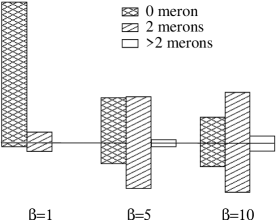
Figure 7: The weight distribution between the sectors with different number of merons at different temperatures for a system with ten spins. The points above (below) the line in the figure correspond to a positive (negative) sign.

We have also done a similar calculation for the spinless fermion model given by Eq. (27). The result for the expectation value of the sign is shown in Fig. 8 as a function of temperature. Two different system sizes are studied, two times two and four times four sites. Also here the average sign appears to decrease exponentially with inverse temperature and system size both in the zero- and two-meron sectors. Asymptotically it seems that the average sign in the zero-meron sector again is increased by a constant factor when leaving out the higher meron sectors.

Figure 8: The average sign as a function of the temperature for the fermion model. The averages are calculated for the zero-meron sector (diamonds) and including the one- and two-meron sector (circles).

We have studied the relative weight of the sectors with different number of merons also for the fermionic system. For the fermions there are configurations with only one meron. This is due to the fact that the empty vertex is given a negative weight and flipping all the loops in a configuration may change the parity of the number of empty vertices. A comparison with exact diagonalization indicates that one only needs to include either the one- or the two-meron sector in addition to the zero-meron sector. In figure 9 the relative weight for the zero-, one-, two-, and higher merons sectors are presented. At high temperatures the relative weight of the zero-meron sector again dominates, while at lower temperatures the weight in the higher meron sectors increases.

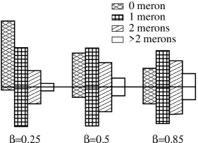
Figure 9: The weight distribution between the sectors with different number of merons at different temperatures for a system with sixteen sites is presented. The points above (below) the line in the figure correspond to a positive (negative) sign.

VII Summary and discussion

We have shown that as long as it is possible to divide the system into independent loops, the meron-cluster approach can be used to decrease the sign problem even when the zero-meron sector is not positive definite. We have applied this method to both frustrated spin systems and spinless fermions. An intermediate regime between a point in parameter space where the meron-cluster algorithm eliminates the sign problem and a point where it cannot be applied is studied. In this intermediate regime the exponential character of the sign problem persists, but one can increase the average sign by a constant factor by limiting measurements to the zero-meron sector. The method is probably of most practical use in the vicinity of points where the sign problem can be eliminated using the meron solution. In a large scale application the weight of the two-meron sector should be decreased by a reweighting techniqueHenelius and Sandvik (2000) to obtain better statistics. To be able to use this algorithm we have combined stochastic series expansion with the concept of directed loops.