Adaptive design of nano-scale dielectric structures for photonics

Abstract

Using adaptive algorithms, the design of nano-scale dielectric structures for photonic applications is explored. Widths of dielectric layers in a linear array are adjusted to match target responses of optical transmission as a function of energy. Two complementary approaches are discussed. The first approach uses adaptive local random updates and progressively adjusts individual dielectric layer widths. The second approach is based on global updating functions in which large subgroups of layers are adjusted simultaneously. Both schemes are applied to obtain specific target responses of the transmission function within selected energy windows, such as discontinuous cut-off or power-law decay filters close to a photonic band edge. These adaptive algorithms are found to be effective tools in the custom design of nano-scale photonic dielectric structures.

I Introduction

In recent years, several types of optical filters, superprisms, and distributed mirrors have been suggested which make use of photon propagation in nano-scale dielectric structures.kosaka ; gralak ; baba While traditional approaches in the design of these devices are based on spatially symmetric arrangements of dielectrics,ohtaka this study explores the merits of intentionally breaking translational symmetry to better realize desired target response profiles, such as transmission or reflection as a function of incident light energy.skorobogatiy It is broken symmetry that enables useful photonic functions. In this paper, two prototype algorithms are discussed which use either local or global progressive updates of dielectric layer widths to match target optical transmission functions, such as a cut-off or a power-law decay filter within a given frequency window.

To illustrate our approach, we focus on the physical problem of one-dimensional arrays of dielectric optical “wells” and “barriers” with alternating refractive indices $n_{1}=1.0$ and $n_{2}=1.5$, respectively. Monochromatic light with energy $E=h\nu$ is incident from the left hand side, and transmission is detected on the right end of the array. The propagation matrix method, keeping track of the boundary conditions on the reflected and transmitted components of the wave function at each individual barrier, is applied to obtain the total transmission coefficient of the array as a function of the photon energy. For the case of a symmetric array with constant barrier width $b(x)=b_{0}=0.5\;\mu m$, shown in Fig. 1(a), this leads to a typical response profile, Fig. 1(b), containing bound state resonances at low energies, and a photonic band edge at $E=0.428\;eV$. The resonances are due to the finite size of the barrier structure. On the other hand, the slightly randomized array with $b(x)=b_{0}\pm\Delta b(x)$ in Fig. 1(c), shows a clear overall reduction of transmission, Fig. 1(d), while still displaying remnant features of the symmetric case, such as the band gap. It is our objective to utilize such intentional translational distortions of symmetric barrier arrays to match target optical response functions, i.e. reflection and transmission, in a given energy window. The optical response of a system with N barrier pairs is determined by the contribution of N-1 barrier poles. Desired filter functions can then be generated over a finite range of energy by adjusting the contribution of each pole.

II Local updates by guided random walk

The first type of adaptive algorithm to achieve this task is based on local random updates of individual barrier widths. These updates are accepted if the resulting transmission profile matches better the target function than the previous one. The basic steps of the algorithm are:

1. Choose target function $T(E)_{target}$ and energy window $E\in[E_{min},E_{max}]$, e.g. cut-off function $T(E)_{target}\equiv\theta(E-E_{c})$ with $E_{c}\in[E_{min},E_{max}]$.

2. Generate initial barrier array by setting length and refractive index of each barrier, for example in a spatially symmetric fashion.

3. Determine $T(E)$ for initial array, and compute its deviation from the target function by evaluating $\Delta=\int_{E_{min}}^{E_{max}}dE[T(E)-T(E)_{target}]^{2}$.

4. Perform a trial random update (change of width) of one barrier (or sets of barriers), and determine $\Delta$ for the following configuration. Additional physical constraints, such as inversion symmetry about the array center, can be enforced in this step.

5. Accept the update if $\Delta$ has decreased with respect to the previous configuration.

6. Repeat random updates of all barriers until acceptable convergence has been reached.

In principle, this annealing approach can be further improved by (i) implementing a Metropolis criterion that avoids local minima in the phase space of barrier widths, and (ii) choosing more updates close to the array boundaries, which affect $T(E)$ the most, than in the vicinity of the center of the structure. In practice, however, the convergence of this algorithm proves to be sufficiently fast. To illustrate this point, let us examine an array of 30+2+30=62 barriers with alternating refractive indices $n_{1}=1.0$ and $n_{2}=1.5$. Perfect inversion symmetry of the barrier widths about the array center is enforced, and the four central barriers are kept unchanged at their initial duty cycles. The reason for this additional constraint is the physical motivation to create an array of adjustable optical barriers that smoothly modulates an incoming free light wave into a crystal Bloch wave through an intermediate layer.

For the symmetric case with a dielectric barrier pair width $d=1\;\mu m$ and an individual barrier width of $b_{0}=0.5\;\mu m$, this array exhibits a band edge at $E_{c}=0.43251\;eV$. This is a natural point in energy to center a target cut-off filter function of the shape $T(E)_{target}\equiv\theta(E-E_{c})$ within a given energy window, which we choose as $E\in[0.35\;eV,0.45\;eV]$. The result of 150 successful updates is displayed in Fig. 2.

In Fig. 2(a) the transmission function for the translationally symmetric array with equal barrier widths $b_{0}$ is shown. It displays characteristic resonances that increase close to the band edge $E_{c}$. Comparing this response with $T(E)$ after the application of the adaptive local random update algorithm, shown in Fig. 2(b), one observes that in both cases the band edge is the dominant feature. However, after convergence to the target filter function, the oscillations in $T(E)$ are largely suppressed within the chosen energy window. The deviation of $T(E)$ from $T(E)_{target}$ is plotted in Fig. 2(c) as a function of accepted updates. From a fit to the form $\Delta_{j}=A\exp{(-j/\chi_{j})}$, where $j$ is the label of successful updates, it is found that this algorithm converges exponentially fast on a scale of $\chi_{j}\approx 27$ updates. After approximately 100 successful updates this function is essentially flat at $\Delta_{\infty}\simeq 0.004\Delta_{0}$, and convergence has been reached. The strength function of the final configuration of barrier widths is displayed in Fig. 2(d). This quantity is defined by $s(x)=2w(x)/d$, where $w(x)$ is the barrier width at position $x$, and $d=1\;\mu m$ is the dielectric barrier pair width. From this last figure it is obvious that the final configuration does not have the simplest spatial symmetry, although inversion symmetry about the array center has been enforced. The barrier widths in the array center remain almost unchanged, whereas they decay rapidly towards the array extremities. Therefore, adjustments in these boundary regions prove to be most effective in achieving a target optical response. Moreover, from this example of multiple independently adjustable barriers (with wells)footnote1 it is evident that there are several sets of possible solutions $\{w(x),x=1,N\}$ for a given finite tolerance $\Delta$. This number of local minima can be reduced by enforcing lower symmetries, such as the inversion about the array center that was used in the above example. However, for more complicated target functions such symmetries may not exist or are not obvious. Furthermore, if fewer symmetries are enforced by hand, there are more adjustable parameters, and the deviation from the target function can be reduced more efficiently. Finally, often practical applications do not require tolerances below the $1\%$-level that is reached by this local random update algorithm.

III Global updates using physical constraints

Let us next turn to an alternative approach to the adaptive design of barrier arrays that it is based on global updates of the strength function $s(x)$. More specifically, the strength function is expanded in a set of basis functions $f_{i}(x)$, $s(x)=\sum_{i=0}^{n}a_{i}f_{i}(x)$, which are subject to the constraints (i) $s(x)=s^{\prime}(x)=0$ at the system boundaries, (ii) $s(L)=1$ and $s^{\prime}(L)=0$ at or close to the array center, and (iii) $s(x)$ is forced to be inversion-symmetric about the array center. The first two constraints are used to determine the lowest four coefficients in the expansion of $s(x)$, i.e. $a_{0}$ up to $a_{3}$. The remaining coefficients $a_{4}$ up to $a_{n}$ are then determined numerically, optimizing the overlap of the transmission in a given energy window with the target function by tuning $\Delta(a_{i})$ with $i=4,...,n$. This approach is only partially numerical. The algorithmic steps can be summarized as follows:

1. Choose target function $T(E)_{target}$ and energy window $[E_{min},E_{max}]$.

2. Generate initial barrier array by setting length and refractive index of each barrier.

3. Determine $T(E)$ for initial array, and compute its deviation from the target function by evaluating $\Delta=\int_{E_{min}}^{E_{max}}dE[T(E)-T(E)_{target}]^{2}$.

4. Expand strength function in a finite basis, e.g. polynomials, and determine lowest four coefficients from boundary conditions.

5. Find minimum of strength function as a function of higher coefficients by numerically minimizing $\Delta(a_{4},....,a_{n})$.

Assuming that the expansion is about a global minimum of $\Delta(a_{n})$, the minimization can be performed sequentially, i.e. by first finding the optimum value of $a^{o}_{4}$ for the expansion to $n=4$, and then optimizing $\Delta(a_{0},...,a_{5})$ for fixed $a^{o}_{4}$, etc. Furthermore, this scheme is improved by adjusting the precise position of the cut-off energy in the target function according to the location of the band edge after each optimization step. In Fig. 3 results for the cut-off target function are shown. The strength function is expanded in a polynomial basis up to $x^{5}$, and boundary conditions are applied to determine the lowest expansion coefficients. The initial parameters are chosen to be identical to the previous discussion of the local random update algorithm.

In Fig. 3(a) the transmission function of the globally adjusted barrier array is shown. Compared with the result of the local random update algorithm, the function looks smoother over the entire energy window, but shows some deviations from the target function in the vicinity of $E_{c}$. It should be noted that in the global update algorithm only two adjustable parameters ($a_{4}$ and $a_{5}$) are considered, whereas there are 30 free parameters widths in the local random scheme. Fig. 3(b) shows the search for a minimum $\Delta(a_{5})$ at an optimum fixed $a_{4}$. For the given expansion, one finds the optimal normalized expansion coefficients $a^{o}_{4}=32.475$ and $a^{o}_{5}=-10.600$ (dotted line), with a minimum total error ($\approx 0.002$) comparable to the local algorithm. The resulting globally adapted strength function is displayed in Fig. 3(c), and in Fig. 3(d) it is compared with the strength function of the local random update algorithm. While these strength functions share the qualitative similarity of a monotonic decay of the barrier widths as the boundaries of the system are approached, obvious differences are that (i) the global update naturally results in a smoother strength function, (ii) this global strength function decays more rapidly at the boundaries, and (iii) it vanishes exactly at the boundaries. These last two features are due to the particular choice of basis functions (polynomials), and the boundary conditions applied to $s(x)$.

Let us conclude the discussion of these two prototype adaptive design algorithms by applying them to less trivial target functions, such as filters with linearly and parabolically decaying transmission within given small energy windows. In Figs. 4(a) and (b) we compare the results of the global and the local update algorithm. The decay from $T(E)=1$ (perfect transmission) to 0 (no transmission) in the target functions (solid line) occurs in a small energy window $E\in[0.42251\;eV,0.44251\;eV]$. It can be seen that for these more complex target responses, the local random update algorithm generally converges better than the global one, because the number of adaptive parameters is much larger for the local method. The present implementation of the global update algorithm is restricted to a two-dimensional search, optimizing the coefficients $a_{4}$ and $a_{5}$. For the target step function filter this method gives better results because here the coefficients $a_{0}$-$a_{5}$ decrease rapidly, and therefore higher-order terms are not needed. In contrast, “smoother” target filter functions require a larger number of coefficients to converge. Therefore, in these cases the results for the global updates are not as good as for the guided random walk because of the restriction to a two-dimensional search. By increasing the number of coefficients in the global update algorithm a solution much closer to the target filter function can be achieved. Naturally, the local random update algorithm is much less sensitive to these differences in the smoothness of the target function, and typically converges fast to an optimal symmetry-breaking configuration within 100 - 200 updates.

IV Conclusions

In summary, we have discussed numerical approaches to design arrays of nano-dielectrics to match desired target functions by intentionally breaking translational symmetry. The global update algorithm is based on an analytical expansion of the strength function of barrier widths in terms of a basis, fixing the leading order expansion coefficients by boundary conditions, and adjusting the remaining ones by numerical optimization. In contrast, the local random update approach uses each barrier width as an adjustable parameter. Sequential updates of barrier widths are performed at random, and the updates are accepted when the resulting transmission profile matches better the target function than the previous one. Refinements of these prototype algorithms are presently being investigated, including combinations of simultaneous local and global updates and enforcement of lesser symmetries, such as point inversion. The broader aim behind these schemes is to develop algorithms that are helpful in designing tools for emerging nanotechnologies.

V Acknowledgments

We are grateful to T. Roscilde for useful discussions, and acknowledge financial support by DARPA, and the Department of Energy, Grant No. DE-FG03-01ER45908.

VI References

H. Kosaka, T. Kawashima, A. Tomita, N. Notomi, T. Tamamura, T. Sato, and S. Kowakami, Phys. Rev. B 58, 10096 (1998).

B. Gralak, S. Enoch, and G. Tayeb, J. Opt. Soc. A. A 17, 1012 (2000).

T. Baba and M. Nakamura, IEEE J. Quant. Elect. 38, 909 (2002).

K. Ohtaka, Phys. Rev. B 19, 5057 (1979).

M. Skorobogatiy and J.D. Joannopoulos, Phys. Rev. B 61, 15554 (2000).

The total number of dielectric layers is 124. The widths of the 4 layers in the center of the system are fixed at their initial values $b_{0}$, as discussed in the text. Since inversion symmetry about the array center is enforced in this example, there remain 60 adjustable widths. Moreover, there is an additional constraint that each pair of barriers satisfies $w_{1}(x)+w_{2}(x)=d$, where the $w_{i}$’s are the respective widths of the on- and off-phase ($n_{1}$ and $n_{2}$), and $d$ is the overall constant width of each dielectric pair. These constraints lead to a reduction of the number of free parameters to 30.

Table of Figures

FIG. 1. Transmission as a function of energy in one-dimensional arrays of 10 optical wells and barriers with alternating refractive indices $n_{1}=1.0$ and $n_{2}=1.5$, respectively. (a) and (b) Symmetric array with barrier widths of $0.5\;\mu m$. (c) and (d) Slightly randomized array with broken translational symmetry. The duty cycle is fixed at $1\;\mu m$, whereas the widths are generated from a uniform random distribution function, centered at $0.5\;\mu m$.
FIG. 2. Adaptive random updates on an array with 30+2+30 optical barrier pairs. (a) Transmission as a function of energy for the translationally symmetric case. (b) Transmission as a function of energy for broken spatial symmetry to achieve a cut-off filter function. (c) Deviation of T(E) from target function. (d) Corresponding strength function.
FIG. 3. Adaptive global updates on an array with 30+2+30 optical barrier pairs. (a) Transmission as a function of energy for broken spatial symmetry to achieve cut-off filter function. (b) Optimization of $\Delta(a_{5})$. (c) Corresponding strength function. (d) Comparison of strength functions for random local (solid line) and global (dashed line) update algorithms.
FIG. 4. Comparison of the adaptive global update and local random update algorithms in a system with 15+2+15 optical barriers. (a) Linear target filter function. (b) Parabolic target filter function. An off-set of $\pm$0.2 has been introduced to simplify the comparison.

Figure 1:

Figure 2:

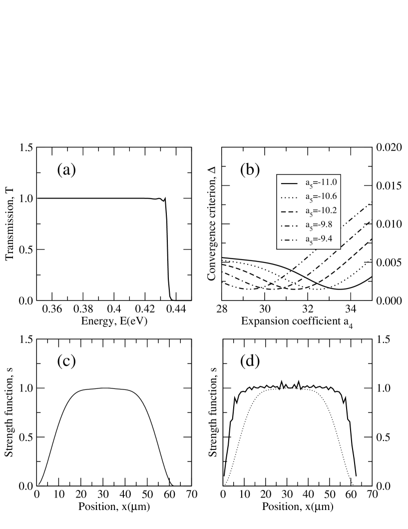
Figure 3:

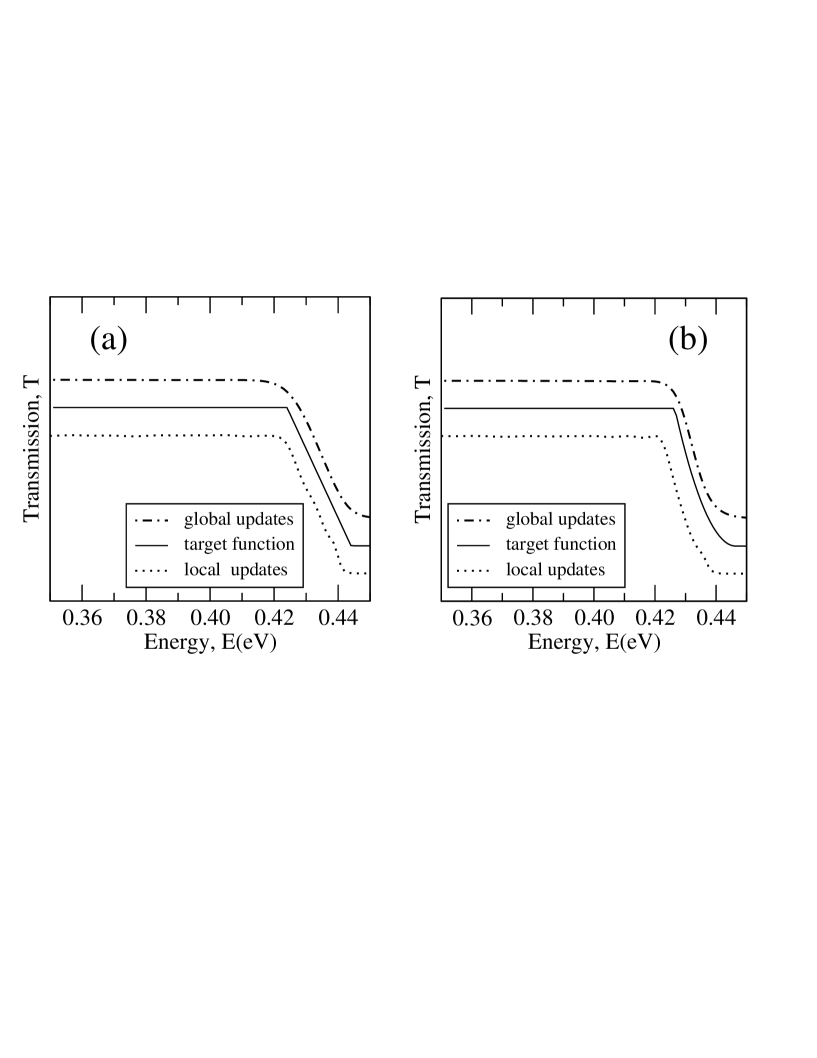
Figure 4: