Dynamics of Conformal Maps for a Class of Non-Laplacian Growth Phenomena

Abstract

Time-dependent conformal maps are used to model a class of growth phenomena limited by coupled non-Laplacian transport processes, such as nonlinear diffusion, advection, and electro-migration. Both continuous and stochastic dynamics are described by generalizing conformal-mapping techniques for viscous fingering and diffusion-limited aggregation, respectively. A general notion of time in stochastic growth is also introduced. The theory is applied to simulations of advection-diffusion-limited aggregation in a background potential flow. A universal crossover in morphology is observed from diffusion-limited to advection-limited fractal patterns with an associated crossover in the growth rate, controlled by a time-dependent effective Péclet number. Remarkably, the fractal dimension is not affected by advection, in spite of dramatic increases in anisotropy and growth rate, due to the persistence of diffusion limitation at small scales.

Laplacian growth models describe some of the best known phenomena of pattern formation far from equilibrium, including continuous dynamics such as viscous fingering bensimon86 and (quasi-static) dendritic solidification  kessler88 and stochastic processes such as diffusion-limited aggregation (DLA) witten81 and dielectric breakdown niemeyer84 . In this class of models, the interfacial velocity is determined by the normal derivative of a harmonic function, so the powerful technique of conformal mapping has been used extensively in two dimensions. Time-dependent conformal maps are used in the classical analysis of continuous Laplacian growth polub45 ; shraiman84 ; feigenbaum01 , and the analogous method of iterated conformal maps has recently been developed for stochastic Laplacian growth hastings98 ; david99 ; hastings01 .

In spite of the broad relevance of these models, real growth phenomena often involve non-Laplacian transport processes, such as advection or electro-migration coupled to diffusion bouissou89 ; argoul95 . Much less theoretical work exists in such cases, in part because conformal mapping would appear to be of little use for non-harmonic functions. An exception is the recent use of streamline coordinates for dendritic solidification in a potential flow, but it turns out that advection has no effect on the shape of an infinite dendrite cummings99 . Stochastic conformal-map dynamics, however, has not yet been formulated for any non-Laplacian transport process (although iterated conformal maps have been used in a recent model of brittle fracture with a bi-harmonic elastic potential levermann02 ).

In this Letter, we formulate the dynamics of conformal maps for growth phenomena limited by non-Laplacian transport processes in a recently identified conformally invariant class bazant03 . We consider both continuous and stochastic growth from a finite seed to allow nontrivial competition between different transport processes. To illustrate the theory, we study fractal growth driven by advection-diffusion in a potential flow.

Transport Processes — Consider a set of scalar ‘fields’, $\mbox{\boldmath{$\phi$}}=\{\phi_{1},\phi_{2},\ldots,\phi_{M}\}$, whose gradients produce quasi-static, conserved ‘flux densities’,

$$\mbox{{\bf F}}_{i}=\sum_{j=1}^{M}C_{ij}\mbox{\boldmath{$\nabla$}}\phi_{j}\ ,\ \ \ \ \mbox{\boldmath{$\nabla$}}\cdot\mbox{{\bf F}}_{i}=0$$ (1)

where the coefficients, $\{C_{ij}(\mbox{\boldmath{$\phi$}})\}$, may be nonlinear functions of the fields. This general system contains a number of physical cases bazant03 : ($M=1$) simple nonlinear diffusion, $\mbox{{\bf F}}_{1}=-D(c)\mbox{\boldmath{$\nabla$}}c$, where $c$ is a temperature or particle concentration and $D(c)$ the diffusivity; ($M=2$) advection-diffusion, $\mbox{{\bf F}}_{1}=-D(c)\mbox{\boldmath{$\nabla$}}c+c\mbox{\boldmath{$\nabla$}}\phi$, of a scalar $c$ in a potential flow, $\mbox{{\bf u}}=\mbox{{\bf F}}_{2}=\mbox{\boldmath{$\nabla$}}\phi$, as well as ionic transport in a supporting electrolyte; and ($M\geq 2$) ionic transport in a neutral electrolyte, $\mbox{{\bf F}}_{i}=-D_{i}(c_{i})\mbox{\boldmath{$\nabla$}}c_{i}-b_{i}(c_{i})q_{i}c_{i}\mbox{\boldmath{$\nabla$}}\phi$, where $c_{i}$, $D_{i}$, $b_{i}$, and $q_{i}$ are respectively the concentration, diffusivity, mobility, and charge of ion $i$, and $\phi$ is the (non-harmonic) electrostatic potential, determined implicitly by electro-neutrality, $\sum_{i=1}^{M}q_{i}c_{i}=0$.

In planar geometries, it is convenient to represent a vector, $\mbox{{\bf F}}=(F_{x},F_{y})$, as a complex scalar, $F=F_{x}+iF_{y}$, so Equation (1) takes the form,

$$F_{i}=\sum_{j=1}^{M}C_{ij}\nabla\phi_{j}\ ,\ \ \ \mbox{Re\hskip 1.0pt}(\overline{\nabla}\mbox{{\bf F}}_{i})=0$$ (2)

in the $z=x+iy$ plane, where $\nabla=\frac{\partial}{\partial x}+i\frac{\partial}{\partial y}$. Under a conformal mapping, $w=f(z)$, $F_{i}$ transforms as

$$F_{i}(z,\bar{z})=\overline{f^{\prime}(z)}\,F_{i}(w,\overline{w}).$$ (3)

(like $\nabla$  needham ), and $\mbox{Re\hskip 1.0pt}(\overline{\nabla}F_{i})=0$ is unchanged. Therefore, even though the solutions (depending on $z$ and $\bar{z}=x-iy$) are not harmonic functions, the usual trick of conformal mapping still works bazant03 : If $\mbox{\boldmath{$\phi$}}(w,\bar{w})$ solves Eq. (2) in one domain, $\Omega_{w}$, then $\mbox{\boldmath{$\phi$}}(f(z),\overline{f(z)})$ solves Eq. (2) in another domain, $\Omega_{z}=f^{-1}(\Omega_{w})$ (with appropriately transformed boundary conditions).

Interfacial dynamics in the plane can be elegantly described by a conformal map, $z=g(w,t)$, from $\Omega_{w}$, the exterior of the unit circle, to $\Omega_{z}(t)$, to the exterior of the (singly connected) growing object polub45 ; shraiman84 ; feigenbaum01 ; hastings98 ; david99 ; hastings01 . Since the map must be univalent (1-1), it has a Laurent series,

$$g(w,t)=A_{1}(t)w+A_{0}(t)+\frac{A_{-1}(t)}{w}+\ldots,\ \ \ |w|>1\ ,$$ (4)

where $A_{1}(t)$ is real and defines an effective diameter of $\Omega_{z}(t)$ hastings98 . As described above, the fields satisfying (1) in $\Omega_{z}(t)$ are easily obtained from the inverse, $w=f(z,t)$, once the same equations are solved in $\Omega_{w}$. As in Laplacian growth, the removal of geometrical complexity from the transport problem is a tremendous simplification.

Boundary Conditions — (BC) Along the moving boundary, $\partial\Omega_{z}(t)$ we consider generalizations of Dirichlet ($\phi_{i}=0$) and Neumann ($\mbox{\boldmath{$\hat{n}$}}\cdot\mbox{\boldmath{$\nabla$}}\phi_{i}=0$) BC  bazant03 :

$$R_{i}\left(\mbox{\boldmath{$\phi$}}(z,\overline{z})\right)=0\ \ \mbox{or}\ \ \mbox{\boldmath{$\hat{n}$}}\cdot\mbox{{\bf F}}_{i}=\mbox{Re\hskip 1.0pt}\left(\overline{n(z)}F_{i}(z,\overline{z})\right)=0,$$ (5)

respectively, for $z\in\partial\Omega_{z}(t)$, where $n=n_{x}+in_{y}$ represents the outward normal, $\hat{n}$, and $R_{i}(\mbox{\boldmath{$\phi$}})$ is a function of the fields. The former BC express interfacial equilibrium for ‘fast reactions’ (compared to transport rates), while the latter expresses impermeability to flows ($\mbox{{\bf F}}=\mbox{{\bf u}}=\mbox{\boldmath{$\nabla$}}\phi$) or flux densities of non-reacting species. Due to Eq. (3), these BC are the same,

$$R_{i}\left(\mbox{\boldmath{$\phi$}}(w,\overline{w})\right)=0\ \ \ \mbox{or}\ \ \ \mbox{\boldmath{$\hat{n}$}}\cdot\mbox{{\bf F}}_{i}=\mbox{Re\hskip 1.0pt}\left(\overline{w}F_{i}(w,\overline{w})\right)=0,$$ (6)

for $w\in\partial\Omega_{w}$, since $n(w)=w=n(z)f^{\prime}(z)/|f^{\prime}(z)|$.

Far from the growth, we assume either constant values of the fields (e.g. temperature, concentration) or given flux (or flow) profiles which drive the growth:

$$\phi_{i}(z,\bar{z})\to\phi_{i}^{\infty}\ \ \ {\mbox{or}}\ \ \ F_{i}(z,\bar{z})\sim F_{i}^{\infty}(z,\bar{z})$$ (7)

as $|z|\to\infty$ (where $F_{i}^{\infty}$ could also vary in time). The former BC also remain the same after conformal mapping, but the latter is transformed by Eqs. (3) and (4):

$$\phi_{i}(w,\bar{w})\to\phi_{i}^{\infty}\ \ \ \ {\mbox{or}}\ \ \ \ F_{i}(w,\bar{w})\sim\overline{A_{1}}F_{i}^{\infty}(A_{1}w,\overline{A_{1}w})$$ (8)

as $|w|\rightarrow\infty$. Through $A_{1}(t)$ $(=\overline{A_{1}}(t))$, the fields and fluxes in $\Omega_{w}$ vary with the diameter of the growth, $\Omega_{z}(t)$.

Continuous Dynamics — Suppose that a Lagrangian boundary point, $z(t)\in\partial\Omega_{z}(t)$, moves in the normal direction with (complex) velocity,

$$v=z_{t}=\alpha\,n\,\sigma,\ \ \ \sigma=\mbox{Re\hskip 1.0pt}(\overline{n}Q)),\ \ \ Q=\sum_{i=1}^{M}B_{i}F_{i},$$ (9)

where Q is a flux density causing growth, $\alpha$ is a constant, and $B_{i}(\mbox{\boldmath{$\phi$}})$ may be functions of the fields. This generalizes Stefan’s law ($\mbox{{\bf v}}=\alpha\,\mbox{\boldmath{$\hat{n}$}}\cdot\mbox{\boldmath{$\nabla$}}\phi$), e.g. to electrodeposition argoul95 (where Q is for the depositing ion).

The classical analysis of viscous fingering is easily generalized to Eqs. (2), (5), (7), and (9). Let $w(t)$ be a ‘marker’ for $z(t)=g(w(t),t)$ on $\Omega_{w}$  feigenbaum01 . Substituting $z_{t}=g^{\prime}\,w_{t}+g_{t}$ into Eq. (9), multiplying by $\overline{wg^{\prime}}$, taking the real part, and using $\mbox{Re\hskip 1.0pt}(\overline{w}w_{t})=0$ for $|w|^{2}=\overline{w}w=1$, we arrive at an evolution equation for the conformal map,

$$\mbox{Re\hskip 1.0pt}(\overline{w\,g^{\prime}}\,g_{t})=\alpha\ \sigma(w,A_{1}(t))\ \ \mbox{ for }\ \ |w|=1$$ (10)

where $\sigma(w,A_{1}(t))=\mbox{Re\hskip 1.0pt}(\overline{w}Q(w,\overline{w}))$ is the normal flux density on $\Omega_{w}$, which depends on $A_{1}(t)$ through Eq. (8).

The evolution equation for radial Laplacian growth (e.g. viscous fingering) polub45 ; shraiman84 , $\mbox{Re\hskip 1.0pt}(\overline{w\,g^{\prime}}\,g_{t})=1$, corresponds to the special case of uniform flux, $\sigma=$ constant. This dynamics is known to preserve number of pole-like singularities (inside the unit circle) for a wide class of initial maps, $g(w,0)$. Except for some elementary maps, e.g. circles and ellipses, which preserve their shapes, arbitrary smooth initial interfaces develop singularities (cusps) in finite time shraiman84 .

In our generalized models, the time-dependent, non-uniform flux, $\sigma$, in Eq. (10) changes the analytic structure of an initial map (e.g. number of poles), so even circles and ellipses become distorted. This raises interesting questions about finite-time singularities, e.g. What is the fate of solidification from a circular seed in a flowing melt (with $\sigma$ described below)? Does advection generally enhance or retard the formation of singularities? We leave these questions for future work and focus here on non-Laplacian fractal growth.

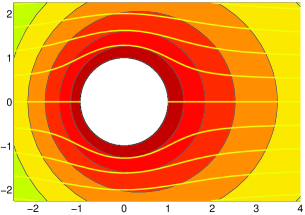
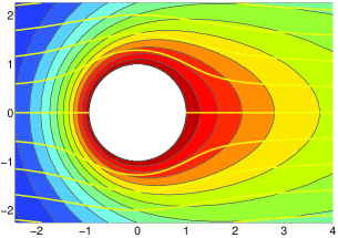
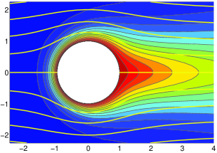
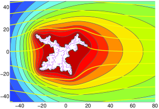
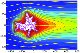
Figure 1: Evolution of the flow (yellow streamlines) and concentration (color contour plot) in $\Omega_{w}$ (top) and in $\Omega_{z}(t)$ (bottom) during advection-diffusion-limited aggregation of $N=10,000$ particles ($\lambda_{o}=L_{o}^{2}=1$) with $\mbox{Pe}_{o}=0.05$. The columns from left to right correspond to $\mbox{Pe\hskip 1.0pt}=0.1$, $\mbox{Pe\hskip 1.0pt}=1$, and $\mbox{Pe\hskip 1.0pt}=10$. The lower plots are shown rescaled by $A_{1}(t_{3})=2$, $A_{1}(t_{193})=20$, and $A_{1}(t_{9621})=200$, the effective diameters of the fractal cluster.

Stochastic Dynamics — Suppose that the domain, $\Omega_{z}(t_{N})$, grows from its initial shape, $\Omega_{z}(0)$, at times $t_{1},t_{2},\ldots,t_{N}$ by discrete ‘bumps’ representing $N$ particles of characteristic area, $\lambda_{o}$  hastings98 ; david99 . Since our models exhibit non-trivial time-dependence (see below), we introduce time into the usual morphological model by replacing Eq. (9) with $p(z,t_{N})=\alpha\,\sigma(z)\,/\lambda_{o}$, for $z\in\partial\Omega_{z}(t_{N-1})$, where $p(z,t_{N})\,|dz|\,dt$ is the probability that the $N$th growth event occurs in the boundary element $(z,z+dz)$ in the time interval $(t,t+dt)$. The waiting time, $t_{N}-t_{N-1}$, is then an exponential random variable with inverse mean,

$$\tau_{N}^{-1}=\frac{\alpha}{\lambda_{o}}\oint_{\partial\Omega_{z}(t_{N-1})}\sigma(z)\,|dz|=\frac{\alpha}{\lambda_{o}}\int_{0}^{2\pi}\sigma(e^{i\theta},A_{1}(t_{N-1}))\,d\theta,$$ (11)

where we use $|dz|=|dw|/|f^{\prime}|$ and $\sigma(z)=|f^{\prime}(z)|\sigma(w)$ from Eq. (3) to transform to $\partial\Omega_{w}$ where $w=e^{i\theta}$ and $|dw|=d\theta$. The probability that the position of the $N$th growth occurs in $(z,z+dz)\subset\partial\Omega_{z}(t_{N-1})$ is, $p_{N}(z)|dz|=\frac{\alpha}{\lambda_{o}}\,\tau_{N}\,\sigma(z)|dz|=P_{N}(\theta)d\theta$, where

$$P_{N}(\theta)=\frac{\alpha}{\lambda_{o}}\,\tau_{N}\,\sigma(e^{i\theta},A_{1}(t_{N-1})),\ \ \ e^{i\theta}\in\Omega_{w}$$ (12)

is the probability measure for angles on the unit circle. In DLA hastings98 , $p_{N}(z)$ is the harmonic measure; $P_{N}(\theta)=(2\pi)^{-1}$ is uniform; and $\tau_{N}$ is not defined.

It is now straightforward to generalize the Hastings-Levitov DLA algorithm hastings98 to our non-Laplacian models. The univalent map $z=g(w,t_{N})$ from $\Omega_{w}$ to $\Omega_{z}(t_{N})$, the exterior of an $N$-particle aggregate, is constructed iteratively from a two-parameter basic map that places a ‘bump’ of area $\lambda_{N}$ around an angle $\theta_{N}$ on the unit circle. In order to fix the area $\lambda_{o}$ of a new bump on $\partial\Omega_{z}(t_{N})$, the size of its pre-image, $\lambda_{N}$, on $\partial\Omega_{w}$ is divided by the Jacobian of the previous map, $\lambda_{k}=\lambda_{o}/|g^{\prime}(e^{i\theta_{N}},t_{N-1})|^{2}$. The first difference with DLA is that the angle, $\theta_{N}$, is chosen according to the time-dependent (non-harmonic) measure, $P_{N}(\theta)$, in Eq. (12). The second difference is the evolving waiting time, $\tau_{N}$, in Eq. (11).

Advection-Diffusion-Limited Aggregation — (ADLA) As an example, we consider the stochastic aggregation of particles around a circular seed of radius, $L_{o}$, limited by advection-diffusion in a uniform potential flow of speed $U$ and concentration $C$. In $\Omega_{z}(t)$ the transport problem has the usual dimensionless form,

$$\mbox{Pe}_{o}\mbox{\boldmath{$\nabla$}}\phi\cdot\mbox{\boldmath{$\nabla$}}c=\mbox{\boldmath{$\nabla$}}^{2}c,\ \ \mbox{\boldmath{$\nabla$}}^{2}\phi=0,\ z\in\Omega_{z}(t)$$ (13)

$$c=0,\ \ \mbox{\boldmath{$\hat{n}$}}\cdot\mbox{\boldmath{$\nabla$}}\phi=0,\ \ \sigma=\mbox{\boldmath{$\hat{n}$}}\cdot\mbox{\boldmath{$\nabla$}}c,\ z\in\partial\Omega_{z}(t)$$ (14)

$$c\to 1,\ \ \mbox{\boldmath{$\nabla$}}\phi\to\mbox{\boldmath{$\hat{x}$}},\ |z|\to\infty$$ (15)

where $x$, $\phi$, $c$, and $\sigma$ are in units of $L_{o}$, $UL_{o}$, $C$, and $DC/L_{o}$, respectively, and $\mbox{Pe}_{o}=UL_{o}/D$ is the initial Péclet number. In complex notation, we solve Eq. (2) in $\Omega_{z}(t)$ with BC (5) and (7) for the ‘fluxes’, $F_{1}=-\mbox{Pe}_{o}\nabla c+c\nabla\phi$ and $F_{2}=u=\nabla\phi$. In $\Omega_{w}$, Equations (2) and (6) are the same, but the BC (7) calls for a background flow speed at $|w|\to\infty$ that diverges with $A_{1}(t)$.

It is natural then to rescale the $w$-velocity by $A_{1}(t)$ to fix the background speed at unity, and instead solve the same equations in $\Omega_{w}$ as in $\Omega_{z}(t)$ with a time-dependent Péclet number, $\mbox{Pe\hskip 1.0pt}(t)=\mbox{Pe}_{o}\,A_{1}(t)$. Since $A_{1}(t)$ is an effective diameter for $\Omega_{z}(t)$, the theory has shown us how to properly define Pe  (which is not obvious for fractals). We also see that advection eventually dominates diffusion since $\mbox{Pe\hskip 1.0pt}(t)\rightarrow\infty$, so we expect to see a crossover from DLA to new advection-limited dynamics, as shown in the simulation of Fig. 1, which we now discuss in detail.

With the scalings above, the velocity potential in $\Omega_{w}$ has the usual harmonic form, $\phi(w)=\mbox{Re\hskip 1.0pt}(w+1/w)$, for potential flow past a cylinder, but the non-harmonic concentration, $c(w,\overline{w},\mbox{Pe\hskip 1.0pt}(t))$, cannot be expressed in terms of elementary functions. However, asymptotic expansions (for fixed $w$) can be derived asympnote ,

$$c(w,\overline{w},\mbox{Pe\hskip 1.0pt})\sim\left\{\begin{array}[]{ll}-\mbox{Re\hskip 1.0pt}\left(\log w/\log\mbox{Pe\hskip 1.0pt}\right)&\ \mbox{Pe\hskip 1.0pt}\ll 1\\ \mbox{erf\hskip 2.0pt}\left[\sqrt{\mbox{Pe\hskip 1.0pt}}\,\mbox{Im\hskip 1.0pt}\left(\sqrt{w}+\frac{1}{\sqrt{w}}\right)\right]&\ \mbox{Pe\hskip 1.0pt}\gg 1\end{array}\right.$$ (16)

The low-Pe  approximation, the familiar harmonic field of Laplacian growth, is valid out to a ‘boundary layer at $\infty$’, while the high-Pe  approximation is valid away from a thin wake on the positive real axis (the branch cut for $\sqrt{w}$) bazant03 . From Eqs. (11), (12), and (16) we also obtain,

$$\tau_{N}\sim\left\{\begin{array}[]{l}-\log\mbox{Pe\hskip 1.0pt}\\ 8\sqrt{\pi/\mbox{Pe\hskip 1.0pt}}\end{array}\right.\ \ \ P_{N}(\theta)\sim\left\{\begin{array}[]{ll}1/2\pi&\ \mbox{Pe\hskip 1.0pt}\ll 1\\ \frac{1}{4}\sin\frac{\theta}{2}&\ \mbox{Pe\hskip 1.0pt}\gg 1\end{array}\right.$$ (17)

where $\tau_{N}$ is measured in units of $(\lambda_{o}/D)/(\alpha C)$. Even for $\mbox{Pe}_{o}\ll 1$, the ADLA dynamics smoothly crosses over from the DLA ‘unstable fixed point’, $\mbox{Pe\hskip 1.0pt}(t)\ll 1$, to a new advection-dominated ‘stable fixed point’, $\mbox{Pe\hskip 1.0pt}(t)\gg 1$, described by Eq. (17).

To investigate this crossover, we accurately obtain the normal flux, $\sigma(w,\mbox{Pe\hskip 1.0pt}(t))$, on $\partial\Omega_{w}$ by interpolating static numerical solutions for a range Pe . Following the methods above, we then perform many ADLA simulations of $N>10^{4}$ particles for various $\mbox{Pe}_{o}$ and $\lambda_{o}/L_{o}^{2}$. Details will be given elsewhere, but here we briefly discuss morphological changes and growth rate.

The Laurent coefficients in Eq. (4) contain morphological information hastings98 ; david99 . As illustrated in Fig. 2, for all $\mbox{Pe}_{o}$, the diameter of the cluster, $A_{1}(t_{N})\sim N^{1/D_{f}}$, remarkably maintains the same fractal dimension as DLA, $D_{f}=1.71$, for all $\mbox{Pe\hskip 1.0pt}(t)$ and $N(t)$ in the scaling regime, $A_{1}(t_{N})\gg 1$. (As a check, we obtain the same $D_{f}$ from the radius of gyration.) A posteriori, this can be understood by noting that the stable fixed point has a growth measure, $P_{N}(\theta)\propto\sin\theta/2$, which is differentiable, and thus locally constant (as in DLA), everywhere except at the rear stagnation point, $\theta=0$. Physically, this simply means that diffusion always dominates advection at small scales. We conjecture that the same $D_{f}$ holds for any non-Laplacian dynamics in our class, if $\lim_{N\rightarrow\infty}P_{N}(\theta)$ is continuous and almost everywhere differentiable. The surprising universality of $D_{f}=1.71$ makes its exact value seem quite fundamental.

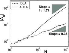
Figure 2: Log-log plot of the Laurent coefficients, $A_{1}(t)$ and $|A_{0}(t)|$ versus $N(t)$, averaged over 30 ADLA simulations ($\mbox{Pe}_{o}=0.05$, $\lambda_{o}=L_{o}^{2}=1$), compared with analogous results for DLA without advection.

Of course, as seen in Fig. 1, the growth is highly anisotropic and moves toward the flow for $\mbox{Pe\hskip 1.0pt}(t)\gg 1$. This is seen in scaling of the next Laurent coefficient, $A_{0}(t)$, the ‘center of charge’ david99 ,

$$|A_{0}(t_{N})|\sim\left\{\begin{array}[]{ll}N^{a}&\ \ \ \mbox{Pe\hskip 1.0pt}\ll 1\\ N^{1/D_{f}}&\ \ \ \mbox{Pe\hskip 1.0pt}\gg 1\end{array}\right.$$ (18)

which crosses over from DLA scaling ($2a=0.7$  david99 ) to the same scaling as $A_{1}(t_{N})$, as shown in Fig. 2. Elsewhere, we will show that $|A_{0}(t)|/A_{1}(t)$ tends to a universal function of $\mbox{Pe\hskip 1.0pt}(t)$ after initial transients vanish, $A_{1}(t)\gg 1$, e.g. $\lim_{t\to\infty}|A_{0}(t)|/A_{1}(t)=0.6$.

The expected total mass versus time, $N(t)$, also undergoes a crossover. Using Eqs. (11) and (17) and integrating $dN/dt=\tau_{N}^{-1}(\mbox{Pe\hskip 1.0pt}(t))=\tau_{N}^{-1}(\mbox{Pe}_{o}N^{1/D_{f}})$ yields, $N(t)\propto t$ for $t\ll 1$ and $N(t)\propto t^{2D_{f}/(2D_{f}-1)}$ for $t\gg 1$, where again only $D_{f}$ matters. The cluster diameter $A_{1}(t)$ switches from $t^{1/D_{f}}$ to $t^{2/(2D_{f}-1)}$ scaling in time, even though the scaling with $N(t)$ does not change. One should also bear in mind that $\tau_{N}\to 0$ as $\mbox{Pe\hskip 1.0pt}(t)\to\infty$, so the quasi-static, discrete-growth approximation must eventually break down (although this is delayed in the dilute limit, $\alpha C\ll 1$).

In summary, we have formulated conformal-map dynamics for a class of planar growth phenomena limited by non-Laplacian transport processes. Although various simplifying assumptions were made, the method enables very efficient simulations of fractal-growth phenomena, such as ADLA, which it seems could not be achieved by more efficient way. By describing competing transport processes, it also paves the way for new studies of general crossover phenomena in pattern formation.

The authors would like to thank M. Ben-Amar, D. Margetis, and T. M. Squires for helpful discussions and ESPCI for support through the Paris Sciences Chair (MZB).

References

- (1) D. Bensimon, L. Kadanoff, B. I. Shraiman, and C. Tang, Rev. Mod. Phys. 58, 977 (1986).
- (2) D. A. Kessler, J. Koplik and H. Levine, Adv. Phys. 37, 255 (1988).
- (3) T. A. Witten and L. M. Sander Phys. Rev. Lett. 47, 1400 (1981).
- (4) L. Niemeyer, L. Pietronero, and H. J. Wiesmann, Phys. Rev. Lett. 52, 1033 (1984).
- (5) P. Ya. Polubarinova-Kochina, Dokl. Akad. Nauk. S. S. S. R. 47, 254 (1945); L. A. Galin, 47, 246 (1945).
- (6) B. I. Shraiman and D. Bensimon, Phys. Rev. A, 30, 2840 (1984).
- (7) M. J. Feigenbaum, I. Procaccia, and B. Davidovitch, J. Stat. Phys. 103, 973 (2001).
- (8) M. Hastings and L. Levitov (1998) Physica D 116, 244 (1998).
- (9) B. Davidovitch, H. G. E. Hentschel, Z. Olami, I. Procaccia, L. M. Sander, and E. Somfai, Phys. Rev. E 59, 1368 (1999).
- (10) M. B. Hastings, Phys. Rev. Lett. 87, 175502 (2001).
- (11) P. Boussiou, B. Perrin, and P. Tabeling, Phys. rev. A 40, 509 (1989); Y.-W. Lee, R. Ananth, and W. N. Gill, J. Crystal Growth 132, 226 (1993).
- (12) F. Argoul and A. Kuhn, Physica A 213, 209 (1995); J. M. Huth, H. L. Swinney, W. D. McCormick, A. Kuhn, and F. Argoul, Phys. Rev. E 51, 3444 (1995).
- (13) L. M. Cummings, Y. E. Hohlov, S. D. Howison, and K. Kornev, J. Fluid Mech. 378, 1 (1999).
- (14) F. Barra, H. G. E. Hentschel, A. Levermann, and I. Procaccia, Phys. Rev. E 65, 045101 (2002).
- (15) M. Z. Bazant, preprint, physics/0302086.
- (16) T. Needham, Visual Complex Analysis (Oxford, 1997).
- (17) D. Margetis and T. M. Squires (private communications).