Variable range hopping and quantum creep in one dimension

Abstract

We study the quantum non linear response to an applied electric field $E$ of a one dimensional pinned charge density wave or Luttinger liquid in presence of disorder. From an explicit construction of low lying metastable states and of bounce instanton solutions between them, we demonstrate quantum creep $v=e^{-c/E^{1/2}}$ as well as a sharp crossover at $E=E^{*}$ towards a linear response form consistent with variable range hopping arguments, but dependent only on electronic degrees of freedom.

Computing the response of a disordered elastic system to an external driving force is a long standing problem. This is of theoretical importance and also relevant for a host of experimental systems, both classical and quantum. For classical systems, typical experimental realizations are domain walls Lemerle et al. (1998); Tybell et al. (2002) and vortex lattice in type II superconductors Blatter et al. (1994); Nattermann and Scheidl (2000). Pinned quantum crystals are charge or spin density waves Grüner (1988), Wigner crystal in two dimensional electron gas Andrei and al. (1988); Willett and et al. (1989) and disordered Luttinger liquids Giamarchi and Orignac (2001). In the absence of quantum or thermal fluctuations disorder leads to pinning or localization. It was initially believed that thermal activation over barriers between pinned states would result Anderson and Kim (1964) in $v(F)\sim\sigma F$ albeit with an exponentially small mobility $\sigma$. However, the glassy nature of such disordered elastic systems leads instead to divergent barriers and to a non linear response Ioffe and Vinokur (1987); Nattermann (1987) of the form $v=\text{exp}(-\beta F^{-\mu})$ known as creep Blatter et al. (1994).

In quantum disordered systems barriers between the many metastable states can be overcome by thermal and quantum activation. Determination of the relation $v(F)$ is thus an even more difficult and mostly open question. Two main issues arise: (i) does one recovers a quantum creep formula at $T=0$ when the system can unpin via quantum tunnelling over barriers; (ii) does one recovers linear response at $T>0$, $v(F)/F\to\sigma$ and what is the $T$ dependence of the conductivity $\sigma$. Although these questions have been answered in details via controlled instanton calculations for pure systems such as the Sine-Gordon model Maki (1977); Hida and Eckern (1984); Hida (1984), with and without dissipation, no controlled method has been found for the disordered problem. Results were obtained using physical arguments for very disordered electronic systems Shklovskii and Efros (1981). The renormalization method used for creep in classical systems Chauve et al. (2000) was extended to quantum problems D. A. Gorokhov and Blatter (2002), but suffers from the same limitations Balents and Le Doussal (2002). The conductivity of charge density waves was studied by Larkin and Lee Larkin and Lee (1978), but only in a strong pinning regime considering tunnelling around single impurities.

In this paper we study the driven quantum dynamics of a pinned 1D charge density wave or of 1D interacting electrons (Luttinger liquid (LL)) in the localized phase, performing a controlled calculation of the tunnelling rates. It is known that this system renormalizes to strong disorder where the (classical) ground state can be found exactly and low lying kink-like excited states constructed. We then study instanton (bounce) solutions and estimate the semiclassical tunnelling rate between these states, in presence of an applied (electric) field. This demonstrates a quantum creep law $v=e^{-c/E^{1/2}}$ at zero temperature. At small non zero temperature we show that a sharp crossover occurs between quantum creep for $E>E^{*}$ and linear response for $E<E^{*}$. The temperature dependence of the conductivity is of the form $\sigma\propto e^{-c/T^{1/2}}$ consistent with Mott’s variable range hopping (VRH) arguments Mott (1990). Applied to the Luttinger liquid, this extends in a precise way the validity of VRH formula to interacting electrons in $d=1$. Note that here contrarily to standard VRH arguments the prefactor $c$ of the temperature dependence in the exponential is determined by the electronic degrees of freedom, and is not dependent in an essential way on coupling to other degrees of freedom such as phonons. This leads to quite different energy scales for $c$ than the standard VRH mechanism.

We consider the Hamiltonian of a charge density wave where the density has a sinusoidal modulation

$$\rho(x)=\rho_{0}\cos(Qx-\phi(x))$$ (1)

where $\phi$ is the phase of the charge density wave. The phase $\phi$ obeys the standard phase action Fukuyama and Lee (1978)

$$\frac{S}{\hbar}=\int_{0}^{L}dx\int_{0}^{\beta\hbar u}dy\frac{1}{2\pi K}\left[(\partial_{y}\phi)^{2}+(\partial_{x}\phi)^{2}\right]$$ (2)

where $u$ is the velocity, $y=u\tau$ and $\beta$ the inverse of the temperature. Furthermore the system has a short distance cutoff (lattice spacing) $\alpha$. The disorder is modelled by a random potential $V(x)$ coupled to the density by $H=-\int dxV(x)\rho(x)$. Assuming that $\phi$ varies slowly at the scale $Q^{-1}$, we can only retain the Fourier components of $V(x)$ close to $Q$ Giamarchi and Schulz (1988). This leads to the action

$$S_{\text{dis}}/\hbar = -\frac{1}{2}\int\frac{dxdyA(x)}{2\pi K\alpha^{2}}e^{i(\phi(x,y)-\zeta(x))}+\text{h.c.}$$ (3)

where we represent the disorder with a random amplitude $A$ and phase $\zeta$, which are both slowly varying variables. For a Gaussian disorder initially, the disorder $\xi(x)=A(x)e^{i\zeta(x)}$ obeys $\overline{\xi(x)\xi(x^{\prime})^{*}}=D\delta(x-x^{\prime})$ other averages are zero. Adding an external electric field $E$ to the system adds to the action

$$S_{E}/\hbar=\int dxdy\tilde{E}\phi(x,y)$$ (4)

with $\tilde{E}=E\rho_{0}/(Qu\hbar)$. The action (2-4) also describes a LL in presence of disorder Giamarchi and Schulz (1988); Giamarchi and Orignac (2001). In that case $Q=2\pi\rho_{0}=2k_{F}$ where $k_{F}$ is the Fermi wavevector for fermions. $K$ is the standard Luttinger parameter that describe the interactions effects ($K=1$ for noninteracting electrons and $K<1$ for repulsive interactions). Our study thus directly gives the conductivity of disordered LLs. In that case the pinning of the phase variable $\phi$ corresponds to the Anderson localization of the system.

At $T=0$ the disorder is a relevant variable. It pins the phase $\phi$. In the ground state the phase $\phi$ varies by a quantity of order $2\pi$ over a distance $\xi_{\text{loc}}$ which is the pinning length of the charge density wave Fukuyama and Lee (1978) or the localization length in the presence of interactions for the interacting particles Giamarchi and Schulz (1988); Giamarchi and Orignac (2001). To determine the dynamics of this model, we renormalize the system up to a point where the disorder is of order one. Since we are interested in the limit of very low temperatures and fields, we can renormalize the action in the absence of $E$ and at $T=0$. The flow in that case is well known Giamarchi and Schulz (1988); Glatz and Nattermann (2002) and we do not reproduce it here. The disorder $D$ scales to strong coupling, and the parameter $K$ decreases. We stop the flow at the lengthscale $l^{*}$ for which $A\sim 1$. At that lengthscale the disorder being of order one, the pinning length is of the order of the lattice spacing $\alpha$. The original localization length of the system is thus $\xi_{\text{loc}}=\alpha e^{l^{*}}$ The electric field is also renormalized and becomes $\frac{2\epsilon}{K^{*}\alpha}=\tilde{E}(l^{*})=\tilde{E}e^{2l^{*}}$ and time and space are rescaled by a factor $e^{-l^{*}}$. In what follows we denote with a star the renormalized quantities at the scale $\xi_{\text{loc}}$. Since $u$ also renormalizes one can absorbs this renormalization by rescaling the time by $u^{*}/u$ which changes $u\to u^{*}$ in all the above expressions.

To study the dynamics we consider (2-4) with the renormalized parameters. Although we stopped the flow when the disorder is of order one we assume that we are truly at strong disorder and can thus consider that the amplitude of the disorder is very large. The main effects thus come from the fluctuations of the random phase of the disorder. In order to perform a semiclassical approximation for the dynamics one must first determine the (classical) ground state of the renormalized system for $E=0$. The disorder being time independent the action is minimized by $\partial_{\tau}\phi=0$. It is convenient to go back to a lattice description. The energy on the lattice is

$$\frac{H}{u^{*}\hbar}=\frac{1}{2\pi K^{*}\alpha}\sum_{i=1}^{N}\left[(\phi_{i+1}-\phi_{i})^{2}-A^{*}\cos(\phi_{i}-\zeta_{i})\right]$$ (5)

with $N=L/\xi_{\text{loc}}$ and we take $-\pi<\zeta_{i}\leq\pi$. Since the renormalized disorder $A^{*}$ in (3) can be considered to be large ($A^{*}=1$), to minimize the cosine term one needs to take $\phi_{i}=\zeta_{i}+2\pi n_{i}$ where $n_{i}$ are integers. The energy becomes

$$\frac{H}{u^{*}\hbar} = \frac{2\pi}{K^{*}\alpha}\sum_{i=1}^{N}\left(n_{i+1}-n_{i}-f_{i}\right)^{2}-\frac{N}{2\pi K^{*}\alpha}$$ (6)

with $f_{i}=(\zeta_{i+1}-\zeta_{i})/(2\pi)$, $-1<f_{i}<1$. Contrarily to higher dimension, here in $d=1$ there is no frustration and one can minimize the action for all bonds simultaneously (i.e. all pairs $\Delta n_{i}=n_{i+1}-n_{i}$) by choosing Glatz (2001):

$$n^{0}_{i}=m_{0}+\sum_{j<i}\left[f_{i}\right]$$ (7)

where $m_{0}$ is an arbitrary integer and $[x]$ denotes the closest integer to $x$. $[x]=0$ if $-1/2<x<1/2$ and $[x]=1$ (resp. $[x]=-1$) for $x>1/2$ (resp $x<-1/2$). The values $[f_{i}]$ thus completely characterize the ground state. Here one takes the $\zeta_{i}$ uniformly distributed, hence the $n^{0}_{i}$ perform a random walk and the ground state has roughness exponent $1/2$ (i.e. $\phi(L)$ scales as $\phi(L)\sim L^{1/2}$) in agreement with other calculations Giamarchi and Le Doussal (1996).

In presence of the electric field $E$ any one of these ground states (with $m_{0}$ fixed) become metastable since the phase $\phi$ wants to increase to gain energy from the field. We estimate the tunnelling rate out of these metastable states if the electric field $E$ is weak. They are given by $P\sim e^{-S^{*}_{B}/\hbar}$ to exponential accuracy, where $S^{*}_{B}$ is the action of a bounce. This is the instanton solution that corresponds to the minimal action needed to go between the two minima and back Coleman (1977); Maki (1977). Such an instanton has the shape of a bubble of typical size $L_{x}$ in the space direction and $L_{\tau}$ in the time direction, and is schematically represented in Fig. 1

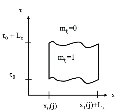
Figure 1: An instanton starting from the ground state where $m_{i,j}=0$ towards a new minimum where $m_{ij}=1$ (see text).

If we denote $i,j$ the coordinate in space and time respectively, then

$$\phi_{ij}=\phi^{0}_{i}+\delta\phi_{ij}=2\pi(n_{i}+m_{ij})+\zeta_{i}$$ (8)

where $\delta\phi_{ij}$ is the deviation from the ground state. We consider unit instantons with $m_{ij}=1$ inside the bubble, and $m_{ij}=0$ outside. The region where $\phi_{ij}$ interpolates between these two values is the wall which encircles the bubble, which is very thin in the large $A^{*}=1$ limit considered here. It is useful to recall that in the pure Sine-Gordon model (obtained here taking all $\zeta_{i}=0$, $n_{i}^{0}=m_{0}$) the bounce instanton solution (with zero friction coefficient) is a circle in the $x,\tau$ plane, since the theory is Lorentz invariant. Here, the surface tension of the instanton walls is highly anisotropic. For a “time-like” wall parallel to the $x$ axis, the surface tension is the same as pure Sine-Gordon (with renormalized parameters) since the disorder is time independant. The corresponding cost in the action is $\sigma_{\tau}L_{x}$ where the line tension of such walls is $\sigma_{\tau}=2\pi/(K^{*}\alpha)$. For a “space-like” wall parallel to the $\tau$ axis the surface tension $\sigma_{x}(i)$ is a random variable. In first approximation the typical instanton now has a rectangular shape, bounded in $x$ by two vertical segments parallel to the $\tau$-axis at coordinates $x=i_{0}$ and $x=i_{0}+L_{x}$, chosen as places where $\sigma_{x}(i)$ is small. The rectangle is closed by two “time-like” segments at $\tau=\tau_{0}$ and $\tau=\tau_{0}+L_{\tau}$.

Let us consider a segment of length $L_{\tau}$ of the wall parallel to the $\tau$ direction between sites $i$ and $i+1$. The extra action due to the presence of the instanton is:

$$\frac{\Delta S}{\hbar}=\frac{2\pi}{K^{*}\alpha}\sum_{j}[m_{i+1,j}^{2}+2m_{i+1,j}(n_{i+1}^{0}-n_{i}^{0}-f_{i})]$$ (9)

Thus, for a unit instanton $m_{i+1,j}=1$, the line tension $\frac{\Delta S}{\hbar}=\sigma_{x}(i)L_{\tau}$, depends on space position $i$:

$$\sigma_{x}(i)=\frac{4\pi}{K^{*}\alpha}g_{i}$$ (10)

with $g_{i}=[f_{i}]-f_{i}+1/2$. One easily sees that $g_{i}$ is uniformly distributed on the interval $[0,1]$. In particular there is a finite weight around $g_{i}=0$ which corresponds to “weak points” in the construction of the ground state where one can bifurcate from point $i$ up to the boundary at low energy cost to a state where the phase is shifted by $2\pi$ on the right of $i$ (or conversely $-2\pi$ on the left of $i$ for the wall on the right). Although these states can be close in energy, the tunnelling rate to them is zero. To obtain a non zero tunnelling rate one must consider “a kink” i.e. tunnelling to a neighboring state where the phase is shifted by $2\pi$ between two walls. This is the tunnelling process described by the above instanton.

The total action cost of the above rectangular instanton is thus:

$$\frac{\Delta S}{\hbar} = (\sigma_{x}(i_{0})+\sigma_{x}(i_{0}+L_{x}))L_{\tau}+2\sigma_{\tau}L_{x}$$ (11)

$$-\frac{4\pi\epsilon L_{x}L_{\tau}}{K^{*}\alpha}$$

Since the two smallest numbers in a set of $L_{x}/\alpha$ random numbers are typically of order $\alpha/L_{x}$ one can estimate $\sigma_{x}(i_{0})+\sigma_{x}(i_{0}+L_{x})\sim\frac{4\pi}{K^{*}\alpha}\frac{\alpha}{L_{x}}$. One then easily estimate the line tension (10) and by minimizing the action (11) get the optimal size for the instanton (for small $\epsilon$)

$$L^{\text{opt}}_{x}=\sqrt{\alpha/\epsilon} \quad,\quad L^{\text{opt}}_{\tau}=1/(2\epsilon)$$ (12)

This yields a decay rate:

$$P \sim e^{-\frac{4\pi}{K^{*}\alpha}\sqrt{\frac{\alpha}{\epsilon}}}=\text{exp}[-\frac{4\sqrt{2}\pi}{(K^{*})^{3/2}}\sqrt{\frac{Q\Delta}{\rho_{0}E\xi_{\text{loc}}}}]$$ (13)

where we have introduced a characteristic energy scale $\Delta=\hbar u^{*}/\xi_{\text{loc}}$ associated with the localization length. Note that $u^{*}/\xi_{\text{loc}}$ is the pinning frequency Fukuyama and Lee (1978). For a simple sine-Gordon theory the dependence is $e^{-\Delta_{M}/(E\xi)}$ and $\Delta_{M}$ is the Mott gap. This expression corresponds to Zener tunnelling across the gap.

Although the above analysis is expected to give correctly the electric field dependence, the precise prefactor in the exponential might be modified by additional physical effects and its precise determination, beyond the crude estimate given here, is delicate. First strictly speaking, in order to reach a stationary state some amount of dissipation should be introduced in the model. This dissipation changes the cost of the time variation of the phase and thus $\sigma_{\tau}$ but does not affect $\sigma_{x}(i)$. It thus slightly changes the prefactor which could in principle be studied as in Hida and Eckern (1984). Next since $\sigma_{x}(i_{0})\neq\sigma_{x}(i_{0}+L_{x})$, the instanton has a lozenge shape and the space like portion can improve its action by taking advantage locally of favorable pins. That may slightly renormalize downwards $\sigma_{\tau}$. Let us also point out that to obtain the response of the system we have computed here a typical instanton, which can occur repeatedly in the volume of the system. There are rarer events that correspond to faster tunnelling. Let us divide the system in intervals of scale $R_{x}\gg L^{\text{opt}}_{x}$ (up to the system size). Within each interval there is typically one place to put two walls separated by $L^{\text{opt}}_{x}$ and for which $(\sigma_{x}(i_{0})+\sigma_{x}(i_{0}+L^{\text{opt}}_{x})\sim 1/R_{x}$. Thus the ground state tunnels (back and forth) with these states at a much faster rate. However since these tunnelling events correspond to special places the density of such atypical kinks being $O(L^{\text{opt}}_{x}/R_{x})$ they cannot lead to a macroscopic current. The system thus stays essentially blocked until the tunnelling events due to the typical instantons can take place. It would however be interesting to see whether such rare events could serve as nucleation center for “quantum avalanches”, which could only increase the creep rate. Although this clearly goes beyond the present study, the explicit construction of the low lying states presented here may allow for a precise study of this faster dynamics, at least numerically.

Let us now see how this quantum creep which corresponds to tunnelling due to quantum effects is modified by the presence of a non zero temperature. Because of the finite temperature the time integration in imaginary time is limited to the finite value $L_{\tau,M}=u^{*}\beta\hbar/(\xi_{\text{loc}}/\alpha)$ (because of the rescaling). This means that the above analysis which was done at $\beta=\infty$ remains valid as long as the size of the bounce in the time direction is smaller than $L_{\tau,M}$. When the size of the bounce reaches the boundary the instanton opens (there are periodic boundary conditions in imaginary time) as shown in Fig. 2.

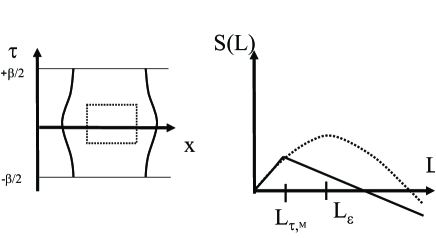
Figure 2: Left: a bounce for large field (dashed line) and at very small fields (solid line). Since the bounce reaches the finite size in imaginary time due to the finite temperature, it opens up. Right : The growth of the action at zero temperatures (dashed line) has a maximum which depends on the electric field. This is the barrier to pass to do the tunnelling. At finite temperature, the barrier decreases very rapidly when the bounce opens up (solid line). The barrier is thus determined essentially by the temperature.

Because there is now no contribution coming from instantons parallel to the space direction, it is easy to see from (11) that the action decreases linearly with the size $L_{x}$ of the instanton. The tunnelling rate is thus fixed by the maximum barrier, i.e. the value of the action when the bounce reaches $L_{\tau,M}$. Because now the maximum barrier is not fixed by the electric field any more, one has to consider both the forward and backward jumps as for the standard TAFF argument Anderson and Kim (1964). The net probability current is thus proportional to

$$J \propto e^{-(S^{*}/\hbar-\epsilon\frac{4\pi L_{\tau,M}^{2}}{K^{*}\alpha})}-e^{-(S^{*}/\hbar+\epsilon\frac{4\pi L_{\tau,M}^{2}}{K^{*}\alpha})}$$ (14)

$$\propto e^{-\frac{S^{*}}{\hbar}}2\sinh(\epsilon\frac{4\pi L_{\tau,M}^{2}}{K^{*}\alpha})$$

where $S^{*}$ is the action of the bounce as given by the saddle point (12) when $L_{\tau}=L_{\tau,M}$. One thus recovers below the crossover field $\epsilon=\xi_{\text{loc}}/(2\beta\hbar\alpha u^{*})$ a linear response, with a conductivity proportional to

$$\sigma(T)\propto e^{-\frac{S^{*}}{\hbar}}=\text{exp}[-\frac{4\pi}{K^{*}}\sqrt{2\beta\Delta}]$$ (15)

Quite remarkably the temperature dependence of the conductivity as obtained by the present formula is identical to Mott’s variable range hopping Mott (1990), where the transition between localized states close in energy is provided by external source of inelastic scattering such as the electron phonon interaction. The important difference between our result and the standard VRH law is that here, inelastic processes are coming from the electron-electron interaction itself (hidden in the existence of the Luttinger liquid parameter $K$). Thus the prefactor in the exponential contains electronic energy scales. The VRH formula contains normally the Debye temperature for phonons. Our result thus lead to a quite different energy scale in the exponential. Although our calculation is done in one dimension only, it is most likely that in higher dimension as well one can obtain similar formulas. Let us note that in one dimension the above instanton picture is very similar physically to the VRH picture, if one remembers that in a Luttinger liquid a kink in $\phi$ is related to the presence of a charge though the formula $\rho=-\nabla\phi/\pi$. Shifting the ground state by one unit is equivalent to moving an electron.