Frequency dependent electrical transport in
the integer quantum Hall effect

Frequency Dependent Electrical Transport
in the Integer Quantum Hall Effect

1 Introduction

It is well established to view the integer quantum Hall effect (QHE) as a sequence of quantum phase transitions associated with critical points that separate energy regions of localised states where the Hall-conductivity $\sigma_{xy}$ is quantised in integer units of $e^{2}/h$ (see, e.g., Huc95 ; SGCS97 ). Simultaneously, the longitudinal conductivity $\sigma_{xx}$ gets unmeasurable small in the limit of vanishing temperature and zero frequency. To check the inherent consequences of this theoretical picture, various experiments have been devised to investigate those properties that should occur near the critical energies $E_{n}$ assigned to the critical points. For example, due to the divergence of the localisation length $\xi(E)\propto|E-E_{n}|^{-\mu}$, the width $\Delta$ of the longitudinal conductivity peaks emerging at the transitions is expected to exhibit power-law scaling with respect to temperature, system size, or an externally applied frequency.

High frequency Hall-conductivity experiments, initially aimed at resolving the problem of the so-called low frequency breakdown of the QHE apparently observed at $\sim 1$ MHz, were successfully carried out at microwave frequencies ($\sim 33$ MHz) KMWS86 . The longitudinal ac conductivity was also studied to obtain some information about localisation and the formation of Hall plateaus in the frequency ranges 100 Hz to 20 kHz LGHS87 and 50–600 MHz BPRT90 . Later, frequency dependent transport has been investigated also in the Gigahertz frequency range below 15 GHz ESKT93 ; BMB98 and above 30 GHz BMKHP98 ; MKBHP98 ; KMK99 .

Dynamical scaling has been studied in several experiments, some of which show indeed power law scaling of the $\sigma_{xx}(\omega)$ peak width as expected, $\Delta\sim\omega^{\kappa}$ ESKT93 ; SET94 ; HZHMDK02 , whereas others do not BMB98 . The exponent $\kappa=(\mu z)^{-1}$ contains both the critical exponent $\mu$ of the localisation length and the dynamical exponent $z$ which relates energy and length scales, $E\sim L^{-z}$. The value of $\mu=2.35\pm 0.03$ is well known from numerical calculations HK90 ; Huc92 , and it also coincides with the outcome of a finite size scaling experiment KHKP91 . However, it is presently only accepted as true that $z=2$ for non-interacting particles, and $z=1$ if Coulomb electron-electron interactions are present LW96 ; YM93 ; HB99 ; WFGC00 ; WX02 . Therefore, a theoretical description of the ac conductivities would clearly contribute to a better understanding of dynamical scaling at quantum critical points.

Legal metrology represents a second area where a better knowledge of frequency dependent transport is highly desirable because the ac quantum Hall effect is applied for the realization and dissemination of the impedance standard and the unit of capacitance, the farad. At the moment the achieved relative uncertainty at a frequency of 1 kHz is of the order $10^{-7}$ which still is at least one order of magnitude to large Del93 ; Del94 ; CHK99 ; SMCHAP02 . It is unclear whether the observed deviations from the quantised dc value are due to external influences like capacitive and inductive couplings caused by the leads and contacts. Alternatively, the measured frequency effects that make exact quantisation impossible could be already inherent in an ideal non-interacting two-dimensional electron gas in the presence of disorder and a perpendicular magnetic field. Of course, applying a finite frequency $\omega$ will lead to a finite $\sigma_{xx}(\omega)$ and in turn will influence the quantisation of $\sigma_{xy}(\omega)$, but it remains to be investigated how large the deviation will be.

Theoretical studies of the ac conductivity in quantum Hall systems started in 1985 Joy85 when it was shown within a semiclassical percolation theory that for finite frequencies the longitudinal conductivity is not zero, thus influencing the quantisation of the Hall-conductivity. The quantum mechanical problem of non-interacting electrons in a 2d disordered system in the presence of a strong perpendicular magnetic field $B$ was tackled by Apel Ape89 using a variational method. Applying an instanton approximation and confining to the high field limit, i.e., restricting to the lowest Landau level (LLL), an analytical solution for the real part of the frequency dependent longitudinal conductivity could be presented, $\sigma_{xx}(\omega)\propto\omega^{2}\ln(1/\omega^{2})$, a result that should hold if the Fermi energy lies deep down in the lower tail of the LLL.

Generalising the above result, both real and imaginary parts of the frequency dependent conductivities were obtained in a sequence of papers by Viehweger and Efetov VE90 ; VE91 ; VE91a . The Kubo conductivities were determined by calculating the functional integrals in super-symmetric representation near non-trivial saddle points. Still, for the final results the Fermi energy was restricted to lie within the energy range of localised states in the lowest tail of the lowest Landau band and, therefore, no proposition for the critical regions at half fillings could be given. The longitudinal conductivity was found to be

$$\sigma_{xx}(\omega)=c\,\omega^{2}\ln^{b}(1/\omega^{2})-{\rm i}e^{2}\omega 2l_{B}^{2}\varrho(E_{\mathrm{F}})\;,$$ (1)

with the density of states $\varrho(E_{\mathrm{F}})$, and two unspecified constants $b$ and $c$ VE90 . The real part of the Hall-conductivity in the same limit was proposed as

$$\sigma_{yx}(\omega)=e^{2}/h\,(\hbar\omega/\Gamma)^{2}\,8\pi l^{2}_{B}n_{e}\;,$$ (2)

where $l_{B}=\sqrt{\hbar/(eB)}$ is the magnetic length, $\Gamma^{2}=\lambda/2\pi l^{2}_{B}$ is the second moment of the white noise disorder potential distribution with disorder strength $\lambda$, and $n_{e}$ denotes the electron density. The deviation due to frequency of the Hall-conductivity from its quantised dc plateau value can be perceived from an approximate expression proposed by Viehweger and Efetov VE91a for the 2nd plateau, e.g., for filling factor $\nu\approx 2$,

$$\sigma_{yx}(\omega)=e^{2}/h\,\Big{[}\frac{2}{1-\omega^{2}/\omega_{c}^{2}}-\Big{(}\frac{2\hbar\omega}{\Gamma}\Big{)}^{2}\,(2-\nu)\Big{]}\;.$$ (3)

Again, $\Gamma$ is a measure of the disorder strength describing the width of the disorder broadened Landau band, and $\omega_{c}=eB/m_{e}$ is the cyclotron frequency with electron mass $m_{e}$. According to (3), due to frequency a deviation from the quantised value becomes apparent even for integer filling.

Before reviewing the attempts which applied numerical methods to overcome the limitations that had to be conceded in connexion with the position of $E_{\mathrm{F}}$ in the analytical work, and to check the permissiveness of the approximations made, it is appropriate here to mention a result for the hopping regime. Polyakov and Shklovskii PS93a obtained for the dissipative part of the ac conductivity a relation which, in contrast to (1), is linear in frequency $\omega$,

$$\Re\,\sigma_{xx}(\omega)=K\,\epsilon\xi\omega\;.$$ (4)

This expression has recently been used to successfully describe experimental data HZH01 . Here, $\xi$ is the localisation length, $\epsilon$ the dielectric constant, and the pre-factor is $K=1/6$ in the limit $\hbar\omega\gg k_{\mathrm{B}}T$. Also, the frequency scaling of the peak width $\Delta\sim\omega^{\kappa}$ was proposed within the same hopping model PS93a .

Turning now to the numerical approaches which were started by Gammel and Brenig who considered the low frequency anomalies and the finite size scaling of the real part of the conductivity peak $\sigma^{p}_{xx}(\omega,L_{y})$ at the critical point of the lowest Landau band GB96 . For these purposes the authors utilised the random Landau model in the high field limit (lowest Landau band only) Huc95 ; HK90 and generalised MacKinnon’s recursive Green function method Mac85 for the evaluation of the real part of the dynamical conductivity. In contrast to the conventional quadratic Drude-like behaviour the peak value decayed linearly with frequency, $\sigma^{p}_{xx}(\omega)=\sigma^{0}_{xx}-\mathrm{const.}\,|\omega|$, which was attributed to the long time tails in the velocity correlations which were observed also in a semiclassical model EB94 ; BGK97 . The range of this unusual linear frequency dependence varied with the spatial correlation length of the disorder potentials. A second result concerns the scaling of $\sigma^{p}_{xx}(\omega,L_{y})$ at low frequencies as a function of the system width $L_{y}$, $\sigma^{p}_{xx}(\omega L^{2}_{y})\propto(\omega L^{2}_{y})^{2-\eta/2}$, where $\eta=2-D(2)=0.36\pm 0.06$ GB96 is related to the multi-fractal wave functions HS92 ; PJ91 ; HKS92 ; Jan94 , and to the anomalous diffusion at the critical point with $\eta\simeq 0.38$ CD88 and $D(2)\simeq 1.62$ HS94 .

The frequency scaling of the $\sigma_{xx}(\omega)$ peak width was considered numerically for the first time in a paper by Avishai and Luck AL96 . Using a continuum model with spatially correlated Gaussian disorder potentials placed on a square lattice, which then was diagonalised within the subspace of functions pertaining to the lowest Landau level, the real part of the dissipative conductivity was evaluated from the Kubo formula involving matrix elements of the velocity of the guiding centres And84a . This is always necessary in single band approximations because of the vanishing of the current matrix elements between states belonging to the same Landau level. As a result, a broadening of the conductivity peak was observed and from a finite size scaling analysis a dynamical exponent $z=1.19\pm 0.13$ could be extracted using $\nu=2.33$ from HK90 . This is rather startling because it is firmly believed that for non-interacting systems $z$ equals the Euclidean dimension of space which gives $z=d=2$ in the QHE case.

A different theoretical approach for the low frequency behaviour of the $\sigma_{xx}(\omega)$ peak has been pursued by Jug and Ziegler JZ99 who studied a Dirac fermion model with an inhomogeneous mass Lea94 applying a non-perturbative calculation. This model leads to a non-zero density of states and to a finite bandwidth of extended states near the centre of the Landau band Zie97 . Therefore, the ac conductivity as well as its peak width do neither show power-law behaviour nor do they vanish in the limit $\omega\to 0$. This latter feature of the model has been asserted to explain the linear frequency dependence and the finite intercept at $\omega=0$ observed experimentally for the width of the conductivity peak by Balaban et al. BMB98 , but, up to now, there is no other experiment showing such a peculiar behaviour.

2 Preliminary considerations – basic relations

In the usual experiments on two-dimensional systems a current $I_{x}(\omega)$ is driven through the sample of length $L_{x}$ and width $L_{y}$. The voltage drop along the current direction, $U_{x}(\omega)$, and that across the sample, $U_{y}(\omega)$, are measured from which the Hall-resistance $R_{\mathrm{H}}(\omega)=U_{y}(\omega)/I_{x}(\omega)=\rho_{xy}(\omega)$ and the longitudinal resistance $R_{x}(\omega)=U_{x}(\omega)/I_{x}(\omega)=\rho_{xx}(\omega)L_{x}/L_{y}$ are obtained, where $\rho_{xy}$ and $\rho_{xx}$ denote the respective resistivities. To compare with the theoretically calculated conductivities one has to use the relations in the following, only in Corbino samples $\sigma_{xx}(\omega)$ can be experimentally detected directly.

The total current through a cross-section, $I_{x}(\omega)=\int_{0}^{L_{y}}j_{x}(\omega,\vec{r})\mathrm{d}y$, is determined by the local current density $j_{x}(\omega,\vec{r})$ which constitutes the response to the applied electric field

$$j_{x}(\omega,\vec{r})=\int\sum_{u\in\{x,y\}}\sigma_{xu}(\omega,\vec{r},\vec{r}^{\prime})E_{u}(\omega,\vec{r}^{\prime})\,\mathrm{d}^{2}\vec{r}^{\prime}\;.$$ (5)

The nonlocal conductivity tensor is particularly important in phase-coherent mesoscopic samples. Usually, for the investigation of the measured macroscopic conductivity tensor one is not interested in its spatial dependence. Therefore, one relies on a local approximation and considers the electric field to be effectively constant. This leads to Ohm’s law $\vec{j}=\widehat{\sigma}\vec{E}$ from which the resistance components are simply given by inverting the conductivity tensor $\widehat{\sigma}$

$$\left(\begin{array}[]{ll}\rho_{xx}&\rho_{xy}\\ \rho_{yx}&\rho_{yy}\end{array}\right)=\frac{1}{\sigma_{xx}\sigma_{yy}-\sigma_{xy}\sigma_{yx}}\ \left(\begin{array}[]{ll}\sigma_{yy}&\sigma_{yx}\\ \sigma_{xy}&\sigma_{xx}\end{array}\right)\;.$$ (6)

For an isotropic system we have $\sigma_{xx}=\sigma_{yy}$ and $\sigma_{yx}=-\sigma_{xy}$ which in case of zero frequency gives the well known relations

$$\rho_{xx}=\frac{\sigma_{xx}}{\sigma_{xx}^{2}+\sigma_{xy}^{2}},\hskip 14.22636pt\rho_{xy}=\frac{-\sigma_{xy}}{\sigma_{xx}^{2}+\sigma_{xy}^{2}}\;.$$ (7)

From experiment one knows that whenever $\rho_{xy}$ is quantised $\rho_{xx}$ gets unmeasurable small which in turn means that $\sigma_{xx}\to 0$ and $\rho_{xy}=1/\sigma_{yx}$. Therefore, to make this happen one normally concludes that the corresponding electronic states have to be localised.

In the presence of frequency this argument no longer holds because electrons in localised states do respond to an applied time dependent electric field giving rise to an alternating current. Also, both real and imaginary parts have to be considered now

$$\sigma_{xx}(\omega)=\sigma^{R}_{xx}(\omega)+{\rm i}\,\sigma^{I}_{xx}(\omega),\hskip 14.22636pt\sigma_{xy}(\omega)=\sigma^{R}_{xy}(\omega)+{\rm i}\,\sigma^{I}_{xy}(\omega)\;.$$ (8)

Assuming an isotropic system, the respective tensor components of the ac resistivity $\rho_{uv}(\omega)=\rho^{R}_{uv}(\omega)+{\rm i}\,\rho^{I}_{uv}(\omega)$ with $u,v\in\{x,y\}$ can be written as

$$\rho^{R}_{uv}(\omega)=\frac{\sigma^{R}_{vu}(\delta\sigma^{2}_{xx}+\delta\sigma^{2}_{xy})+2\sigma^{I}_{vu}(\sigma^{R}_{xx}\,\sigma^{I}_{xx}+\sigma^{R}_{xy}\,\sigma^{I}_{xy})}{(\delta\sigma^{2}_{xx}+\delta\sigma^{2}_{xy})^{2}+4(\sigma^{R}_{xx}\,\sigma^{I}_{xx}+\sigma^{R}_{xy}\,\sigma^{I}_{xy})^{2}}$$ (9)

$$\rho^{I}_{uv}(\omega)=\frac{\sigma^{I}_{vu}(\delta\sigma^{2}_{xx}+\delta\sigma^{2}_{xy})+2\sigma^{R}_{uv}(\sigma^{R}_{xx}\,\sigma^{I}_{xx}+\sigma^{R}_{xy}\,\sigma^{I}_{xy})}{(\delta\sigma^{2}_{xx}+\delta\sigma^{2}_{xy})^{2}+4(\sigma^{R}_{xx}\,\sigma^{I}_{xx}+\sigma^{R}_{xy}\,\sigma^{I}_{xy})^{2}}$$ (10)

with the abbreviations $\delta\sigma^{2}_{xx}\equiv(\sigma^{R}_{xx})^{2}-(\sigma^{I}_{xx})^{2}$ and $\delta\sigma^{2}_{xy}\equiv(\sigma^{R}_{xy})^{2}-(\sigma^{I}_{xy})^{2}$.

3 Model and Transport theory

We describe the dynamics of non-interacting particles moving within a two-dimensional plane in the presence of a perpendicular magnetic field and random electrostatic disorder potentials by a lattice model with Hamiltonian

$$H=\sum_{\vec{r}}w_{\vec{r}}|\vec{r}\rangle\langle\vec{r}|-\sum_{<\vec{r}\neq\vec{r^{\prime}}>}V_{\vec{r}\vec{r^{\prime}}}|\vec{r}\rangle\langle\vec{r^{\prime}}|\;.$$ (11)

The random disorder potentials associated with the lattice sites are denoted by $w_{\vec{r}}$ with probability density distribution $P(w_{\vec{r}})=1/W$ within the interval $[-W/2,W/2]$, where $W$ is the disorder strength, and the $|\vec{r}\rangle$ are the lattice base vectors. The transfer terms

$$V_{\vec{r}\vec{r^{\prime}}}=V\exp\big{(}-{\rm i}\,e^{2}/\hbar\int_{\vec{r}}^{\vec{r^{\prime}}}\vec{A}(\vec{l})\,\mathrm{d}\vec{l}\,\big{)}\;,$$ (12)

which connect only nearest neighbours on the lattice, contain the influence of the applied magnetic field via the vector potential $\vec{A}(\vec{r})=(0,Bx,0)$ in their phase factors. $V$ and the lattice constant $a$ define the units of energy and length, respectively.

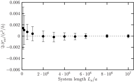
Figure 1: Disorder averaged imaginary part of $\widetilde{\sigma}^{\ast}_{xx}(E,\omega,\varepsilon)$ at energy $E/V=-3.35$, frequency $\hbar\omega/V=0.001$, and $\varepsilon/V=0.0008$ as a function of sample length $L_{x}=Na$. The system width is $L_{y}/a=32$ and the number of realisations amounts to 29 for $L_{x}/a\leq 5\cdot 10^{6}$ and to 8 for larger lengths

The electrical transport is calculated within linear response theory using the Kubo formula which allows to determine the time dependent linear conductivity from the current matrix elements of the unperturbed system

$$\sigma_{uv}(E_{\mathrm{F}},T,\omega) = \frac{\pi e^{2}}{\Omega}\int_{-\infty}^{\infty}\!\mathrm{d}E\frac{f(E)-f(E+\hbar\omega)}{\omega}$$

$${}\times\mathrm{Tr}\big{\{}\hat{v}_{u}\delta(E_{\mathrm{F}}-H)\hat{v}_{v}\delta(E_{\mathrm{F}}+\hbar\omega-H)\big{\}}\;,$$

where $f(E)=(\exp[(E-E_{\mathrm{F}})/(k_{\mathrm{B}}T)]-1)^{-1}$ is the Fermi function. The area of the system is $\Omega=L_{x}L_{y}$, $\hat{v}_{u}={\rm i}/\hbar[H,u]$ signifies the $u$-component of the velocity operator, and $\delta(E+\hbar\omega-H)={\rm i}/(2\pi)(G^{\omega,+}(E)-G^{\omega,-}(E))$, where $G^{\omega,\pm}(E)=((E+\hbar\omega\pm{\rm i}\varepsilon)\mathrm{I}-H)^{-1}$ is the resolvent with imaginary frequency ${\rm i}\varepsilon$ and unit matrix $\mathrm{I}$.

For finite systems at temperature $T=0$ K, ensuring the correct order of limits for size $\Omega$ and imaginary frequency ${\rm i}\varepsilon$, one gets with $\gamma=\omega+2{\rm i}\varepsilon/\hbar$

$$\sigma_{uv}(E_{\mathrm{F}},\omega) = \lim_{\varepsilon\rightarrow 0}\lim_{\Omega\rightarrow\infty}\frac{e^{2}}{h}\frac{1}{\Omega\hbar\omega}\Bigg{[}\int_{E_{F}-\hbar\omega}^{E_{F}}\mathrm{d}E\,{\rm Tr}\,\Big{\{}(\hbar\gamma)^{2}\,[uG^{\omega,+}vG^{-}]$$ (15)

$${}-(\hbar\omega)^{2}\,[uG^{\omega,+}vG^{+}]+\,2{\rm i}\varepsilon\,[uv(G^{\omega,+}-G^{-})]\Big{\}}$$

$${}-\int_{-\infty}^{E_{F}-\hbar\omega}\mathrm{d}E\,{\rm Tr}\Big{\{}(\hbar\omega)^{2}\,[uG^{\omega,+}vG^{+}-uG^{\omega,-}vG^{-}]\Big{\}}\Bigg{]}$$

$$= \lim_{\varepsilon\rightarrow 0}\lim_{\Omega\rightarrow\infty}\frac{e^{2}}{h}\frac{1}{\Omega\hbar\omega}\Bigg{[}\int_{E_{F}-\hbar\omega}^{E_{F}}\widetilde{\sigma}_{uv}(E,\omega,\varepsilon,L_{x},L_{y})\,\mathrm{d}E$$

$${}+\int_{-\infty}^{E_{F}-\hbar\omega}\widetilde{\sigma}^{\ast}_{uv}(E,\omega,\varepsilon,L_{x},L_{y})\,\mathrm{d}E\Bigg{]}\;.$$

Figure 2: The variance of $\langle\Im\,\widetilde{\sigma}^{\ast}_{xx}(E,\omega,\varepsilon)\rangle$ versus system length $L_{x}$ calculated for the averages shown in Fig. 1 exhibiting an empirical power-law $\sim L_{x}^{0.5}$

One can show that the second integral with the limits ($-\infty,E_{\mathrm{F}}-\hbar\omega$) does not contribute to the real part of $\sigma_{uv}(E_{\mathrm{F}},\omega)$ because the kernel is identical zero, but we were not able to proof the same also for the imaginary part. Therefore, using the recursive Green function method explained in the next section, we numerically studied $\Im\,\widetilde{\sigma}^{\ast}_{uv}(E,\omega,\varepsilon,L_{x},L_{y})$ and found it to become very small only after disorder averaging. As an example we show in Fig. 1 the dependence of $\langle\Im\,\widetilde{\sigma}^{\ast}_{xx}\rangle$, averaged over up to 29 realisations, on the length of the system for a particular energy $E/V=-3.35$ and width $L_{y}/a=32$. Also the variance of $\langle\widetilde{\sigma}^{\ast}_{xx}(E,\omega,\varepsilon)\rangle$ gets smaller with system length following an empirical power law $\sim(L_{x}/a)^{-0.5}$ (see Fig. 2). In what follows we neglect the second integral for the calculation of the imaginary parts of the conductivities and assume that only the contribution of the first one with limits ($E_{\mathrm{F}}-\hbar\omega,E_{\mathrm{F}}$) matters. Of course, on has to be particularly careful even if the kernel is very small because with increasing disorder strength the energy range that contributes to the integral (finite density of states) tends to infinity. Therefore, a rigorous proof for the vanishing of this integral kernel is highly desirable.

4 Recursive Green function method

A very efficient method for the numerical investigation of large disordered chains, strips and bars that are assembled by successively adding on slice at a time has been pioneered by MacKinnon Mac80 . This iterative technique relies on the property that the Hamiltonian $H^{(N+1)}$ of a lattice system containing $N+1$ slices, each a lattice constant $a$ apart, can be decomposed into parts that describe the system containing $N$ slices, $H^{(N)}$, the next slice added, $H_{N+1,N+1}$, and a term that connects the last slice to the rest, $H^{\prime}_{N}=H_{N,N+1}+H_{N+1,N}$. Then the corresponding resolvent is formally equivalent to the Dyson equation $G=G_{0}+G_{0}\widehat{V}G$ where the ‘unperturbed’ $G_{0}$ represents the direct sum of $H^{(N)}$ and $H_{N+1,N+1}$, and $\widehat{V}$ corresponds to the ‘interaction’ $H^{\prime}_{N}$. The essential advantage of this method is the fact that, for a fixed width $L_{y}$, the system size is increased in length adding slice by slice, whereas the size of the matrices to be dealt with numerically remains the same Mac80 ; MK83 .

A number of physical quantities like localisation length MK81 ; MK82 ; SKM84 ; KPS01 , density of states SKM84 ; KSM84 , and some dc transport coefficients Mac85 ; SKM85 ; VRSM00 have been calculated by this technique over the years. Also, this method was implemented for the evaluation of the real part of the ac conductivity in 1d SKK83 ; Sas84 and 2d systems GB96 ; Gam94 ; GE99 . Further efforts to included also the real and imaginary parts of the Hall- and the imaginary part of the longitudinal conductivity in quantum Hall systems were also successfully accomplished BS99 ; BS01 ; BS02 .

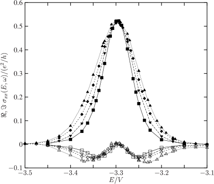
Figure 3: The real and imaginary parts of $\sigma_{xx}(E,\omega)$ as a function of energy and frequency $\hbar\omega/V=2\cdot 10^{-4}$ ( ), $5\cdot 10^{-4}$ (▼), $1\cdot 10^{-3}$ (

 

), $2\cdot 10^{-3}$ (▲). For comparison, the cyclotron frequency is $\hbar\omega_{c}\approx 1.57\,V$ for $\alpha_{B}=1/8$ which was chosen for the magnetic flux density. The disorder strength is $W/V=1$ and the maximal system width amounts to $L_{y}/a=96$ with periodic boundary conditions applied

The iteration equations of the resolvent matrix acting on the subspace of such slices with indices $i,j\leq N$ in the $N$-th iteration step can be written as

$$G_{i,j}^{\omega,\pm,(N+1)} = G_{i,j}^{\omega,\pm,(N)}+G_{i,N}^{\omega,\pm,(N)}\,H_{N,N+1}\,G_{N+1,N+1}^{\omega,\pm,(N+1)}\,H_{N+1,N}\,G_{N,j}^{\omega,\pm,(N)}$$

$$G_{N+1,N+1}^{\omega,\pm,(N+1)} = [(E+\hbar\omega\pm{\rm i}\varepsilon){\rm I}-H_{N+1,N+1}-H_{N+1,N}G_{N,N}^{\omega,\pm,(N)}H_{N,N+1}]^{-1}$$

$$G_{i,N+1}^{\omega,\pm,(N+1)} = G_{i,N}^{\omega,\pm,(N)}\,H_{N,N+1}\,G_{N+1,N+1}^{\omega,\pm,(N+1)}$$

$$G_{N+1,j}^{\omega,\pm,(N+1)} = G_{N+1,N+1}^{\omega,\pm,(N+1)}\,H_{N+1,N}\,G_{N,j}^{\omega,\pm,(N)}\;.$$ (16)

The calculation of the ac conductivities starts with the Kubo formula (15) by setting up a recursion equation for fixed energy $E$, width $L_{y}=Ma$, and imaginary frequency $\varepsilon$, which, e.g., for the longitudinal component reads

$$\widetilde{\sigma}_{xx}(E,\omega,\varepsilon,N) = \frac{e^{2}}{hMNa^{2}}S_{N}^{xx}=\frac{e^{2}}{hMNa^{2}}\mathrm{Tr}\bigg{\{}\sum_{i,j}^{N}\Big{[}(\hbar\gamma)^{2}x_{i}G_{ij}^{\omega,+}x_{j}G_{ji}^{-}$$ (17)

$${}-(\hbar\omega)^{2}x_{i}G_{ij}^{\omega,+}x_{j}G_{ji}^{+}+2{\rm i}\varepsilon\delta_{ij}x_{i}^{2}(G_{ij}^{\omega,+}-G_{ji}^{-})\Big{]}\bigg{\}}\;.$$

The iteration equation for adding a new slice is given by

$$S_{N+1}^{xx} = S_{N}^{xx}+{\rm Tr}\big{\{}A_{N}R_{N+1}^{-}+D_{N}^{1}R_{N+1}^{\omega,+}D_{N}^{2}R_{N+1}^{-}$$ (18)

$${}+B_{N}R_{N+1}^{\omega,+}-D_{N}^{3}R_{N+1}^{+}D_{N}^{4}R_{N+1}^{\omega,+}-C_{N}R_{N+1}^{+}\big{\}}\;.$$

with $R_{N+1}^{\omega,\pm}\equiv G_{N+1,N+1}^{\omega,\pm,(N+1)}$, and a set of auxiliary quantities as defined in the appendix. The coupled iteration equations and the auxiliary quantities are evaluated numerically, the starting values are set to be zero. In addition, coordinate translations are required in each iteration step to keep the origin $x_{N+1}=0$ which then guarantees the numerical stability.

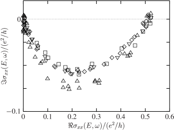
Figure 4: The imaginary part of $\sigma_{xx}(E,\omega)$ as a function of the real part. Data are taken from Fig. 3

5 Longitudinal conductivity $\sigma_{xx}(E,\omega)$

In this section we present our numerical results of the longitudinal conductivity as a function of frequency for various positions of the Fermi energy within the lowest Landau band. The real and imaginary parts of $\sigma_{xx}(E_{\mathrm{F}},\omega)$ were calculated for several frequencies, but, for the sake of legibility, only four of them are plotted in Fig. 3 versus energy. While the real part exhibits a positive single Gaussian-like peak with maximum $\approx 0.5\,e^{2}/h$ at the critical energy, the imaginary part, which is negative almost everywhere, has a double structure and vanishes near the critical point. $\Im\,\sigma_{xx}(E_{\mathrm{F}},\omega)$ almost looks like the modulus of the derivative of the real part with respect to energy. Plotting $\Im\,\sigma_{xx}(E_{\mathrm{F}},\omega)$ as a function of $\Re\,\sigma_{xx}(E_{\mathrm{F}},\omega)$ (see Fig. 4) we obtain for frequencies $\omega<\omega^{\ast}$ a single, approximately semi-circular curve that, up to a minus sign, closely resembles the experimental results of Hohls et al. HZH01 . However, for larger $\omega$ our data points deviate from a single curve.

Figure 5: The real ($\bullet$) and imaginary ( ) part of $\sigma_{xx}(E_{\mathrm{F}},\omega)$ in units of $e^{2}/h$ at $E_{\mathrm{F}}/V=-3.5$ as a function of frequency. Further parameters are the disorder strength $W/V=1.0$, system width $L_{y}/a=32$ and $\varepsilon/V=0.0004$

5.1 Frequency dependence of real and imaginary parts

The behaviour of the real and imaginary part of the longitudinal ac conductivity in the lower tail of the lowest Landau band ($E/V=-3.5$) is shown in Fig. 5. We find for the imaginary part a linear frequency dependence for small $\omega$ which is, apart from a minus sign, in accordance with (1) VE90 . The real part can nicely be fitted to $\propto\omega^{2}\log^{2}[V/(\hbar\omega)]^{2}$ in conformance with (1) and $b=2$, but disagrees with the findings in Ape89 where $b=1$ was proposed.

5.2 Behaviour of the maximum of $\sigma_{xx}(\omega)$

The frequency dependence of the real part of the longitudinal conductivity peak value was already investigated in GB96 where for long-range correlated disorder potentials a non-Drude-like decay was observed. We obtained a similar behaviour also for spatially uncorrelated disorder potentials in a lattice model BS01 . In Fig. 6 the difference $|\Re\,\sigma^{\mathrm{p}}_{xx}(\omega)-\sigma^{\mathrm{p}}_{xx}(0)|$ is plotted versus frequency in a double logarithmic plot from which a linear relation can be discerned. A linear increase with frequency was found for the imaginary part of the longitudinal conductivity at the critical point as well BS01 . The standard explanation for the non-Drude behaviour in terms of long time tails in the velocity correlations, which were shown to exist in a QHE system GB96 ; BGK97 , seems not to be adequate in our case. For the uncorrelated disorder potentials considered here, it is not clear whether the picture of electron motion along equipotential lines, a basic ingredient for the arguments in GB96 , is appropriate.

Figure 6: The non-Drude decrease of the peak value of the longitudinal conductivity as a function of frequency. A linear behaviour of $|\Re\,\sigma^{\mathrm{p}}_{xx}(\omega)-\sigma^{\mathrm{p}}_{xx}(0)|$ is clearly observed with $\sigma^{\mathrm{p}}_{xx}(0)/(e^{2}/h)=0.512$ using the following parameters $E/V=-3.29$, $W/V=0.1$, $L_{y}/a=32$, $\varepsilon/V=0.0004$

Figure 7: Frequency scaling of the $\sigma_{xx}(\omega)$ peak width. The width in energy $\Delta E$ ($\Box$) and the width in filling factor $\Delta\nu$ ($\diamond$) show a power-law $\Delta\sim\omega^{\kappa}$ with an exponent $\kappa=(\mu z)^{-1}=0.21$

5.3 Scaling of the $\sigma_{xx}(\omega)$ peak width

The scaling of the width of the conductivity peaks with frequency is shown in Fig. 7 where both the $\sigma_{xx}(\omega)$ peak width expressed in energy and, due to the knowledge of the density of states, in filling factor are shown to follow a power-law $\Delta\sim\omega^{\kappa}$ with $\kappa=(\mu z)^{-1}=0.21$ BS99 . Taking $\mu=2.35$ from Huc92 we get $z=2.026$ close to what is expected for non-interacting electrons. Therefore, the result reported in AL96 seems to be doubtful. However, spatial correlations in the disorder potentials as considered in AL96 may influence the outcome. Alternatively, one could fix $z=2$ and obtain $\mu=2.38$ in close agreement with the results from numerical calculations of the scaling of the static conductivity GB94 or the localisation length Huc92 .

The experimentally observed values $\kappa\simeq 0.42$ ESKT93 and $\kappa=0.5\pm 0.1$ HZHMDK02 are larger by a factor of about 2. This is usually attributed to the influence of electron-electron interactions ($z=1$) which were neglected in the numerical investigations.

   

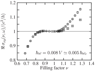
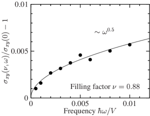
Figure 8: Frequency dependent Hall-conductivity: The figure on the l.h.s shows $\sigma_{xy}(\omega)$ versus filling factor for two system sizes $L_{y}/a=64$ ($\circ$) and $L_{y}/a=128$ ($\Box$). On the r.h.s., the relative deviation of the Hall-conductivity from the dc value, $\sigma_{xy}(\omega)/\sigma_{xy}(0)-1$, is plotted as a function of frequency for $\nu=0.88$

6 Frequency dependent Hall-conductivity

The Hall-conductivity due to an external time dependent electric field as a function of filling factor $\nu$ is shown in Fig. 8 for system widths $L_{y}/a=64$ and $L_{y}/a=128$, respectively. While $\sigma_{xy}(\omega)$ has already converged for $E_{\mathrm{F}}$ lying in the upper tail of the lowest Landau band a pronounced shift can be seen in the lower tail of the next Landau band. For $\nu=1.3$ a system width of at least $L_{y}/a=192$ was necessary for $\sigma_{xy}(\omega)$ to converge. This behaviour originates in the exponential increase of the localisation length with increasing Landau band index. Due to the applied frequency $\hbar\omega/V=0.008$ the $\sigma_{xy}$ plateau is not flat, but rather has a parabola shape near the minimum at $\nu=1.0$, similar to what has been observed in experiment SMCHAP02 . An example of the deviation of $\sigma_{xy}(\omega)$ from its quantised dc value is shown on the right hand side of Fig. 8 where $\sigma_{xy}(\omega)/\sigma_{xy}(0)-1$ is plotted versus frequency for filling factor $\nu=0.88$. A power-law curve $\sim\omega^{0.5}$ can be fitted to the data points. Using this empirical relation, we find a relative deviation of the order of $5\cdot 10^{-6}$ when extrapolated down to to 1 kHz, the frequency usually applied in metrological experiments Del93 ; Del94 ; CHK99 ; SMCHAP02 . Therefore, there is no quantisation in the neighbourhood of integer filling even in an ideal 2d electron gas without contacts, external leads, and other experimental imperfections. Recent calculations, however, show that this deviation can be considerably reduced, even below $1\cdot 10^{-8}$, if spatially correlated disorder potentials are considered in the model Sch03 .

7 Conclusions

The frequency dependent electrical transport in integer quantum Hall systems has been reviewed and the various theoretical developments have been presented. Starting from a linear response expression a method has been demonstrated which is well suited for the numerical evaluation of the real and imaginary parts of both the time dependent longitudinal and the Hall-conductivity. In contrast to the analytical approaches, no further approximations or restrictions such as the position of the Fermi energy have to be considered.

We discussed recent numerical results in some detail with particular emphasis placed on the frequency scaling of the peak width of the longitudinal conductivity emerging at the quantum critical points, and on the quantisation of the ac Hall-conductivity at the plateau. As expected, the latter was found to depend on the applied frequency. The extrapolation of our calculations down to low frequencies resulted in a relative deviation of $5\cdot 10^{-6}$ at $\sim 1\,$kHz when spatially uncorrelated disorder potentials are considered. Disorder potentials with spatial correlations, likely to exist in real samples, will probably reduce this pronounced frequency effect.

Our result for the frequency dependence of the $\sigma_{xx}$ peak width showed power-law scaling, $\Delta\sim\omega^{\kappa}$, where $\kappa=(\mu z)^{-1}=0.21$ as expected for non-interacting electrons. Therefore, electron-electron interactions have presumably to be taken into account to explain the experimentally observed $\kappa\approx 0.5$ Also, the influence of the spatial correlation of the disorder potentials may influence the value of $\kappa$.

The frequency dependences of the real and imaginary parts of the longitudinal conductivities, previously obtained analytically for Fermi energies lying deep down in the lowest tail of the lowest Landau band, have been confirmed by our numerical investigation. However, the quadratic behaviour found at low frequencies for the real part of $\sigma_{xx}(\omega)$ has to be contrasted with the linear frequency dependence that has been proposed for hopping conduction.

Finally, a non-Drude decay of the $\sigma_{xx}$ peak value with frequency, $\sigma^{p}_{xx}(0)-\sigma^{\mathrm{p}}_{xx}(\omega)\propto\omega$, as reported earlier for correlated disorder potentials, has been observed also in the presence of uncorrelated disorder potentials. A convincing explanation for the latter behaviour is still missing.

Appendix

The iteration equations of the auxiliary quantities (required in (18)) can be written as BS02 with $V_{N}\equiv H_{N,N+1}=H^{\dagger}_{N+1,N}$

$$A_{N+1} = V_{N+1}^{{\dagger}}R_{N+1}^{-}\big{[}A_{N}+D_{N}^{1}R_{N+1}^{\omega,+}D_{N}^{2}\big{]}R_{N+1}^{-}V_{N+1}$$ (19)

$$B_{N+1} = V_{N+1}^{{\dagger}}R_{N+1}^{\omega,+}\big{[}B_{N}-D_{N}^{3}R_{N+1}^{+}D_{N}^{4}+D_{N}^{2}R_{N+1}^{-}D_{N}^{1}\big{]}R_{N+1}^{\omega,+}V_{N+1}$$ (20)

$$C_{N+1} = V_{N+1}^{{\dagger}}R_{N+1}^{+}\big{[}C_{N}+D_{N}^{4}R_{N+1}^{\omega,+}D_{N}^{3}\big{]}R_{N+1}^{+}V_{N+1}$$ (21)

$$F_{N+1} = V_{N+1}^{{\dagger}}R_{N+1}^{\omega,+}\big{[}F_{N}+D_{N}^{3}R_{N+1}^{+}D_{N}^{4}\big{]}R_{N+1}^{\omega,+}V_{N+1}$$ (22)

$$G_{N+1} = V_{N+1}^{{\dagger}}R_{N+1}^{-}\big{[}G_{N}+D_{N}^{10}R_{N+1}^{\omega,-}D_{N}^{11}\big{]}R_{N+1}^{-}V_{N+1}$$ (23)

$$H_{N+1} = V_{N+1}^{{\dagger}}R_{N+1}^{\omega,-}\big{[}H_{N}+D_{N}^{11}R_{N+1}^{-}D_{N}^{10}\big{]}R_{N+1}^{\omega,-}V_{N+1}$$ (24)

$$D_{N+1}^{1} = V_{N+1}^{{\dagger}}R_{N+1}^{-}D_{N}^{1}R_{N+1}^{\omega,+}V_{N+1}$$ (25)

$$D_{N+1}^{2} = V_{N+1}^{{\dagger}}R_{N+1}^{\omega,+}D_{N}^{2}R_{N+1}^{-}V_{N+1}$$ (26)

$$D_{N+1}^{3} = V_{N+1}^{{\dagger}}R_{N+1}^{\omega,+}D_{N}^{3}R_{N+1}^{+}V_{N+1}$$ (27)

$$D_{N+1}^{4} = V_{N+1}^{{\dagger}}R_{N+1}^{+}D_{N}^{4}R_{N+1}^{\omega,+}V_{N+1}$$ (28)

$$D_{N+1}^{5} = V_{N+1}^{{\dagger}}R_{N+1}^{-}D_{N}^{5}R_{N+1}^{-}V_{N+1}$$ (29)

$$D_{N+1}^{6} = V_{N+1}^{{\dagger}}R_{N+1}^{+}D_{N}^{6}R_{N+1}^{+}V_{N+1}$$ (30)

$$D_{N+1}^{10} = V_{N+1}^{{\dagger}}R_{N+1}^{-}D_{N}^{10}R_{N+1}^{\omega,-}V_{N+1}$$ (31)

$$D_{N+1}^{11} = V_{N+1}^{{\dagger}}R_{N+1}^{\omega,-}D_{N}^{11}R_{N+1}^{-}V_{N+1}$$ (32)

$$D_{N+1}^{14} = V_{N+1}^{{\dagger}}R_{N+1}^{\omega,-}D_{N}^{14}R_{N+1}^{\omega,-}V_{N+1}$$ (33)

$$D_{N+1}^{15} = V_{N+1}^{{\dagger}}R_{N+1}^{\omega,+}D_{N}^{15}R_{N+1}^{\omega,+}V_{N+1}$$ (34)

$$D_{N+1}^{16} = V_{N+1}^{{\dagger}}R_{N+1}^{-}D_{N}^{16}R_{N+1}^{-}V_{N+1}$$ (35)

$$E_{N+1}^{1} = V_{N+1}^{{\dagger}}R_{N+1}^{+}\Big{(}E_{N}^{1}+(\hbar\omega)I\Big{)}R_{N+1}^{+}V_{N+1}$$ (36)

$$E_{N+1}^{2} = V_{N+1}^{{\dagger}}R_{N+1}^{-}\Big{(}E_{N}^{2}+(\hbar\omega)I\Big{)}R_{N+1}^{-}V_{N+1}$$ (37)

$$E_{N+1}^{3} = V_{N+1}^{{\dagger}}R_{N+1}^{\omega,+}\Big{(}E_{N}^{3}+(\hbar\omega)I\Big{)}R_{N+1}^{\omega,+}V_{N+1}$$ (38)

$$E_{N+1}^{4} = V_{N+1}^{{\dagger}}R_{N+1}^{\omega,-}\Big{(}E_{N}^{4}+(\hbar\omega)I\Big{)}R_{N+1}^{\omega,-}V_{N+1}\;,$$ (39)

where the auxiliary quantities are defined by

$$A_{N} = V_{N}^{{\dagger}}\bigg{(}\sum_{i,j}^{N}G_{Ni}^{-}x_{i}\big{[}(\hbar\gamma)^{2}G_{ij}^{\omega,+}-2{\rm i}\varepsilon\delta_{ij}{\rm I}\big{]}x_{j}G_{jN}^{-}\bigg{)}V_{N}$$ (40)

$$B_{N} = V_{N}^{{\dagger}}\bigg{(}\sum_{i,j}^{N}G_{Ni}^{\omega,+}x_{i}\big{[}(\hbar\gamma)^{2}G_{ij}^{-}+2{\rm i}\varepsilon\delta_{ij}{\rm I}+(\hbar\omega)^{2}G_{ij}^{+}\big{]}x_{j}G_{jN}^{\omega,+}\bigg{)}V_{N}$$ (41)

$$C_{N} = V_{N}^{{\dagger}}\bigg{(}\sum_{i,j}^{N}(\hbar\omega)^{2}G_{Ni}^{+}x_{i}G_{ij}^{\omega,+}x_{j}G_{jN}^{+}\bigg{)}V_{N}$$ (42)

$$F_{N} = V_{N}^{{\dagger}}\bigg{(}\sum_{i,j}^{N}(\hbar\omega)^{2}G_{Ni}^{\omega,+}x_{i}G_{ij}^{+}x_{j}G_{jN}^{\omega,+}\bigg{)}V_{N}$$ (43)

$$G_{N} = V_{N}^{{\dagger}}\bigg{(}\sum_{i,j}^{N}(\hbar\omega)^{2}G_{Ni}^{-}x_{i}G_{ij}^{\omega,-}x_{j}G_{jN}^{-}\bigg{)}V_{N}$$ (44)

$$H_{N} = V_{N}^{{\dagger}}\bigg{(}\sum_{i,j}^{N}(\hbar\omega)^{2}G_{Ni}^{\omega,-}x_{i}G_{ij}^{-}x_{j}G_{jN}^{\omega,-}\bigg{)}V_{N}$$ (45)

$$D_{N}^{1} = V_{N}^{{\dagger}}\bigg{(}\sum_{i}^{N}(\hbar\gamma)G_{Ni}^{-}x_{i}G_{iN}^{\omega,+}\bigg{)}V_{N}$$ (46)

$$D_{N}^{2} = V_{N}^{{\dagger}}\bigg{(}\sum_{i}^{N}(\hbar\gamma)G_{Ni}^{\omega,+}x_{i}G_{iN}^{-}\bigg{)}V_{N}$$ (47)

$$D_{N}^{3} = V_{N}^{{\dagger}}\bigg{(}\sum_{i}^{N}(\hbar\omega)G_{Ni}^{\omega,+}x_{i}G_{iN}^{+}\bigg{)}V_{N}$$ (48)

$$D_{N}^{4} = V_{N}^{{\dagger}}\bigg{(}\sum_{i}^{N}(\hbar\omega)G_{Ni}^{+}x_{i}G_{iN}^{\omega,+}\bigg{)}V_{N}$$ (49)

$$D_{N}^{5} = V_{N}^{{\dagger}}\bigg{(}\sum_{i}^{N}(\hbar\omega)G_{Ni}^{-}x_{i}G_{iN}^{-}\bigg{)}V_{N}$$ (50)

$$D_{N}^{6} = V_{N}^{{\dagger}}\bigg{(}\sum_{i}^{N}(\hbar\omega)G_{Ni}^{+}x_{i}G_{iN}^{+}\bigg{)}V_{N}$$ (51)

$$D_{N}^{10} = V_{N}^{{\dagger}}\bigg{(}\sum_{i}^{N}(\hbar\omega)G_{Ni}^{-}x_{i}G_{iN}^{\omega,-}\bigg{)}V_{N}$$ (52)

$$D_{N}^{11} = V_{N}^{{\dagger}}\bigg{(}\sum_{i}^{N}(\hbar\omega)G_{Ni}^{\omega,-}x_{i}G_{iN}^{-}\bigg{)}V_{N}$$ (53)

$$D_{N}^{14} = V_{N}^{{\dagger}}\bigg{(}\sum_{i}^{N}(\hbar\omega)G_{Ni}^{\omega,-}x_{i}G_{iN}^{\omega,-}\bigg{)}V_{N}$$ (54)

$$D_{N}^{15} = V_{N}^{{\dagger}}\bigg{(}\sum_{i}^{N}(\hbar\omega)G_{Ni}^{\omega,+}x_{i}G_{iN}^{\omega,+}\bigg{)}V_{N}$$ (55)

$$D_{N}^{16} = V_{N}^{{\dagger}}\bigg{(}\sum_{i}^{N}(\hbar\omega)G_{Ni}^{-}x_{i}G_{iN}^{-}\bigg{)}V_{N}$$ (56)

$$E_{N}^{1} = V_{N}^{{\dagger}}\bigg{(}\sum_{i}^{N}(\hbar\omega)G_{Ni}^{+}G_{iN}^{+}\bigg{)}V_{N}$$ (57)

$$E_{N}^{2} = V_{N}^{{\dagger}}\bigg{(}\sum_{i}^{N}(\hbar\omega)G_{Ni}^{-}G_{iN}^{-}\bigg{)}V_{N}$$ (58)

$$E_{N}^{3} = V_{N}^{{\dagger}}\bigg{(}\sum_{i}^{N}(\hbar\omega)G_{Ni}^{\omega,+}G_{iN}^{\omega,+}\bigg{)}V_{N}$$ (59)

$$E_{N}^{4} = V_{N}^{{\dagger}}\bigg{(}\sum_{i}^{N}(\hbar\omega)G_{Ni}^{\omega,-}G_{iN}^{\omega,-}\bigg{)}V_{N}\;.$$ (60)

For the translation of the coordinates $x_{i}\to x_{i}-a$ one gets

$$A_{N}^{{}^{\prime}} = A_{N}+H_{N}^{1}-2aD_{N}^{5}+a^{2}E_{N}^{2}+aH_{N}^{3}$$ (61)

$$B_{N}^{{}^{\prime}} = B_{N}+H_{N}^{2}-H_{N}^{1}+a(H_{N}^{4}-H_{N}^{3})$$ (62)

$$C_{N}^{{}^{\prime}} = C_{N}+H_{N}^{2}-2aD_{N}^{6}+a^{2}E_{N}^{1}+aH_{N}^{4}$$ (63)

$$F_{N}^{{}^{\prime}} = F_{N}-aD_{N}^{4}+2aD_{N}^{15}-aD_{N}^{3}-aH_{N}^{4}-a^{2}E_{N}^{3}$$ (64)

$$G_{N}^{{}^{\prime}} = G_{N}+a(D_{N}^{10}+D_{N}^{11})-2aD_{N}^{16}+a^{2}E_{N}^{2}+aH_{N}^{5}$$ (65)

$$H_{N}^{{}^{\prime}} = H_{N}-aD_{N}^{10}+2aD_{N}^{14}-aD_{N}^{11}-aH_{N}^{5}-a^{2}E_{N}^{4}$$ (66)

$$D_{N}^{1/2^{\prime}} = D_{N}^{1/2}+H_{N}^{3}$$ (67)

$$D_{N}^{3/4^{\prime}} = D_{N}^{3/4}+H_{N}^{4}$$ (68)

$$D_{N}^{5^{\prime}} = D_{N}^{5}-aE_{N}^{2}$$ (69)

$$D_{N}^{6^{\prime}} = D_{N}^{6}-aE_{N}^{1}$$ (70)

$$D_{N}^{10/11^{\prime}} = D_{N}^{10/11}+H_{N}^{5}$$ (71)

$$D_{N}^{14^{\prime}} = D_{N}^{14}-aE_{N}^{4}$$ (72)

$$D_{N}^{15^{\prime}} = D_{N}^{15}-aE_{N}^{3}$$ (73)

$$D_{N}^{16^{\prime}} = D_{N}^{16}-aE_{N}^{2}\;,$$ (74)

with the following abbreviations

$$H_{N}^{1} = a(D_{N}^{1}+D_{N}^{2})$$ (75)

$$H_{N}^{2} = a(D_{N}^{3}+D_{N}^{4})$$ (76)

$$H_{N}^{3} = aV_{N}^{{\dagger}}(R_{N}^{\omega,+}-R_{N}^{-})V_{N}$$ (77)

$$H_{N}^{4} = aV_{N}^{{\dagger}}(R_{N}^{\omega,+}-R_{N}^{+})V_{N}$$ (78)

$$H_{N}^{5} = aV_{N}^{{\dagger}}(R_{N}^{\omega,-}-R_{N}^{-})V_{N}\;.$$ (79)

References

• (1) B. Huckestein: Rev. Mod. Phys. 67, 357 (1995)
• (2) S. L. Sondhi, S. M. Girvin, J. P. Carini, D. Shahar: Rev. Mod. Phys. 69(1), 315 (1997)
• (3) F. Kuchar, R. Meisels, G. Weimann, W. Schlapp: Phys. Rev. B 33(4), 2956 (1986)
• (4) J. I. Lee, B. B. Goldberg, M. Heiblum, P. J. Stiles: Solid State Commun. 64(4), 447 (1987)
• (5) I. E. Batov, A. V. Polisskii, M. I. Reznikov, V. I. Tal’yanskii: Solid State Commun. 76(1), 25 (1990)
• (6) L. W. Engel, D. Shahar, C. Kurdak, D. C. Tsui: Phys. Rev. Lett. 71(16), 2638 (1993)
• (7) N. Q. Balaban, U. Meirav, I. Bar-Joseph: Phys. Rev. Lett. 81(22), 4967 (1998)
• (8) W. Belitsch, R. Meisels, F. Kuchar, G. Hein, K. Pierz: Physica B 249–251, 119 (1998)
• (9) R. Meisels, F. Kuchar, W. Belitsch, G. Hein, K. Pierz: Physica B 256-258, 74 (1998)
• (10) F. Kuchar, R. Meisels, B. Kramer: Advances in Solid State Physics 39, 231 (1999)
• (11) D. Shahar, L. W. Engel, D. C. Tsui: In High Magnetic Fields in the Physics of Semiconductors, edited by D. Heiman (World Scientific Publishing Co., Singapore, 1995): pp. 256–259
• (12) F. Hohls, U. Zeitler, R. J. Haug, R. Meisels, K. Dybko, F. Kuchar: cond-mat/0207426 (2002)
• (13) B. Huckestein, B. Kramer: Phys. Rev. Lett. 64(12), 1437 (1990)
• (14) B. Huckestein: Europhysics Letters 20(5), 451 (1992)
• (15) S. Koch, R. J. Haug, K. v. Klitzing, K. Ploog: Phys. Rev. Lett. 67, 883 (1991)
• (16) D.-H. Lee, Z. Wang: Phys. Rev. Lett. 76(21), 4014 (1996)
• (17) S.-R. E. Yang, A. H. MacDonald: Phys. Rev. Lett. 70(26), 4110 (1993)
• (18) B. Huckestein, M. Backhaus: Phys. Rev. Lett. 82(25), 5100 (1999)
• (19) Z. Wang, M. P. A. Fisher, S. M. Girvin, J. T. Chalker: Phys. Rev. B 61(12), 8326 (2000)
• (20) Z. Wang, S. Xiong: Phys. Rev. B 65, 195316 (2002)
• (21) F. Delahaye: J. Appl. Phys. 73, 7914 (1993)
• (22) F. Delahaye: Metrologia 31, 367 (1994/95)
• (23) S. W. Chua, A. Hartland, B. P. Kibble: IEEE Trans. Instrum. Meas. 48, 309 (1999)
• (24) J. Schurr, J. Melcher, A. von Campenhausen, G. Hein, F.-J. Ahlers, K. Pierz: Metrologia 39, 3 (2002)
• (25) R. Joynt: J. Phys. C: Solid State Phys. 18, L331 (1985)
• (26) W. Apel: J. Phys.: Condens. Matter 1, 9387 (1989)
• (27) O. Viehweger, K. B. Efetov: J. Phys.: Condens. Matter 2(33), 7049 (1990)
• (28) O. Viehweger, K. B. Efetov: J. Phys.: Condens. Matter 3(11), 1675 (1991)
• (29) O. Viehweger, K. B. Efetov: Phys. Rev. B 44(3), 1168 (1991)
• (30) D. G. Polyakov, B. I. Shklovskii: Phys. Rev. B 48(15), 11167 (1993)
• (31) F. Hohls, U. Zeitler, R. J. Haug: Phys. Rev. Lett. 86(22), 5124 (2001)
• (32) B. M. Gammel, W. Brenig: Phys. Rev. B 53(20), R13279 (1996)
• (33) A. MacKinnon: Z. Phys. B 59, 385 (1985)
• (34) F. Evers, W. Brenig: Z. Phys. B 94, 155 (1994)
• (35) W. Brenig, B. M. Gammel, P. Kratzer: Z. Phys. B 103, 417 (1997)
• (36) B. Huckestein, L. Schweitzer: In High Magnetic Fields in Semiconductor Physics III: Proceedings of the International Conference, Würzburg 1990, edited by G. Landwehr (Springer Series in Solid-State Sciences 101, Springer, Berlin, 1992): pp. 84–88
• (37) W. Pook, M. Janßen: Z. Phys. B 82, 295 (1991)
• (38) B. Huckestein, B. Kramer, L. Schweitzer: Surface Science 263, 125 (1992)
• (39) M. Janßen: International Journal of Modern Physics B 8(8), 943 (1994)
• (40) J. T. Chalker, G. J. Daniell: Phys. Rev. Lett. 61(5), 593 (1988)
• (41) B. Huckestein, L. Schweitzer: Phys. Rev. Lett. 72(5), 713 (1994)
• (42) Y. Avishay, J. M. Luck: preprint, cond-mat/9609265 (1996)
• (43) T. Ando: J. Phys. Soc. Jpn. 53(9), 3101 (1984)
• (44) G. Jug, K. Ziegler: Phys. Rev. B 59(8), 5738 (1999)
• (45) A. W. W. Ludwig, M. P. A. Fisher, R. Shankar, G. Grinstein: Phys. Rev. B 50, 7526 (1994)
• (46) K. Ziegler: Phys. Rev. B 55(16), 10661 (1997)
• (47) A. MacKinnon: J. Phys. C 13, L1031 (1980)
• (48) A. MacKinnon, B. Kramer: Z. Phys. B 53, 1 (1983)
• (49) A. MacKinnon, B. Kramer: Phys. Rev. Lett. 47(21), 1546 (1981)
• (50) A. MacKinnon, B. Kramer: In Lecture Notes in Physics, edited by G. Landwehr (Springer-Verlag, Berlin, Heidelberg, New York, Tokyo, 1982): pp. 74–86
• (51) L. Schweitzer, B. Kramer, A. MacKinnon: J. Phys. C 17, 4111 (1984)
• (52) T. Koschny, H. Potempa, L. Schweitzer: Phys. Rev. Lett. 86(17), 3863 (2001)
• (53) B. Kramer, L. Schweitzer, A. MacKinnon: Z. Phys. B - Condensed Matter 56, 297 (1984)
• (54) L. Schweitzer, B. Kramer, A. MacKinnon: Z. Phys. B 59, 379 (1985)
• (55) C. Villagonzalo, R. A. Römer, M. Schreiber, A. MacKinnon: Phys. Rev. B 62, 16446 (2000)
• (56) T. Saso, C. I. Kim, T. Kasua: J. Phys. Soc. Jap. 52, 1888 (1983)
• (57) T. Saso: J. Phys. C 17, 2905 (1984)
• (58) B. M. Gammel: Ph. D. Thesis (Technical-University Munich) (1994)
• (59) B. M. Gammel, F. Evers: unpublished report, 10 pages (1999)
• (60) A. Bäker, L. Schweitzer: Ann. Phys. (Leipzig) 8, SI-21 (1999)
• (61) A. Bäker, L. Schweitzer: In Proc. 25th Int. Conf. Phys. Semicond., Osaka 2000, edited by N. Miura, T. Ando (Springer, Berlin, 2001): vol. 78 of Springer Proceedings in Physics: pp. 975–976
• (62) A. Bäker, L. Schweitzer: PTB-report, unpublished, 94 pages (2002)
• (63) B. M. Gammel, W. Brenig: Phys. Rev. Lett. 73(24), 3286 (1994)
• (64) L. Schweitzer: to be published (2003)