Limit cycle induced by multiplicative noise in a system of coupled Brownian motors

Abstract

We study a model consisting of $N$ nonlinear oscillators with global periodic coupling and local multiplicative and additive noises. The model was shown to undergo a nonequilibrium phase transition towards a broken-symmetry phase exhibiting noise-induced “ratchet” behavior. A previous study [10] focused on the relationship between the character of the hysteresis loop, the number of “homogeneous” mean-field solutions and the shape of the stationary mean-field probability distribution function. Here we show –as suggested by the absence of stable solutions when the load force is beyond a critical value– the existence of a limit cycle induced by both: multiplicative noise and global periodic coupling.

I Introduction

The study of dynamical systems has shown that limit cycles are ubiquitous in a wide range of physical applications [1, 2]. From a physicist’s point of view, limit cycles are thought of as a way to balance the in- and out- energy flows. Even when those flows are not oscillatory in time, a system’s oscillatory motion can occur equalizing such flows over one period. A nice pedagogical example of such a process, based on a perturbative analysis of the nonlinear van der Pol oscillator, can be found in [3]. As is well known, limit cycles are robust –structurally stable under small perturbations– attractors in dissipative systems without external oscillations [1, 2]. Usually, limit cycles arise in dynamical systems described by ordinary differential equations (ODE) [1, 2], but there are several examples where such kind of cycles also arise in partial differential equations (PDE) or “extended systems”, as for instance, in the ”brusselator” model for the so called “chemical clocks” [4, 5].

Limit cycles arise also in systems with noise. Noise or fluctuations, that are present everywhere, have been generally considered as a factor that destroys order. However, a wealth of investigations on nonlinear physics during the last decades have shown numerous examples, both in zero- and higher dimensional systems, of nonequilibrium systems where noise plays an “ordering” role. In such cases, the transfer of concepts from equilibrium thermodynamics, in order to study phenomena away from equilibrium, is not always adequate and many times is misleading. Some examples of such nonequilibrium phenomena are: noise induced unimodal-bimodal transitions in some zero dimensional models (describing either concentrated systems or uniforms fields) [6], shifts in critical points [7], stochastic resonance in zero-dimensional and extended systems [8, 9], noise-delayed decay of unstable states [10], noise-induced spatial patterns [11], noise induced phase transitions in extended systems [12], etc.

Here, we discuss an extended system described by PDE’s, where noise plays a key role in controlling and inducing a limit cycle. The model that we analyze here is the one used in [13, 14] to study a ratchet-like transport mechanism arising through a symmetry breaking, noise–induced, nonequilibrium phase transition. In a recent paper [15] a system with a noise induced phase transition, based on a model that is a variant of Kuramoto’s model for coupled phase oscillators [16]; was analyzed. In addition to the phenomenon of anomalous hysteresis, evidence of the existence of a limit cycle for a given parameter region; is also shown.

The model we analyze consists of a system of periodically coupled nonlinear phase oscillators with a multiplicative white noise. Coupled oscillators have been used to model systems with collective dynamics exhibiting plenty of interesting properties like equilibrium and nonequilibrium phase transitions, coherence, synchronization, segregation and clustering phenomena. In this particular model a ratchet-like transport mechanism arises through a symmetry breaking, noise–induced, nonequilibrium phase transition [13], produced by the simultaneous effect of coupling between the oscillators and the presence of a multiplicative noise. The symmetry breaking does not arise in the absence of any of these two ingredients. In [13] it was also shown that the current, as a function of a load force $F$, produces an anomalous (clockwise) hysteresis cycle. Recently we have reported that, changing the multiplicative noise intensity $Q$ and/or the coupled constant $K_{0}$, a transition from anomalous to normal (counter-clockwise) hysteresis is produced [14]. The result was obtained exploiting a mean field approximation. The transition curve in the plane $(K_{0},Q)$, separating the region where the hysteresis cycle is anomalous from the one where it is normal, was clearly determined.

Here we focus on the time behavior. We use a method for detecting the existence of a limit cycle based on the evaluation of the distance between two solutions separated by a (fixed) time interval [17]. In this way, we not only show the existence of a limit cycle for $F>F_{c}$ (with $F_{c}$ a loading threshold value), but also determine its period. We also found the time dependence of the probability distribution function along the cycle and calculate the order parameter of the model vs. $t$, clearly showing the limit cycle. Next, we gain insight into its origin through the study of the large coupling limit ($K_{0}\to\infty$). Finally, we draw some conclusions.

II The model, mean field and the method used

For completeness we present a brief description of our model, which is similar to the one used in Refs. [13] and [14]. We consider a set of globally coupled stochastic differential equations (to be interpreted in the sense of Stratonovich) for N degrees of freedom (phases) $X_{i}(t)$

$$\dot{X}_{i}=-\frac{\partial U_{i}}{\partial X_{i}}+\sqrt{2T}\,\xi_{i}(t)-\frac{1}{N}\sum_{j=1}^{N}K(X_{i}-X_{j}).$$ (1)

This model can be visualized (at least for some parameter values) as a set of overdamped interacting pendulums. The second term in Eq. (1) considers the effect of thermal fluctuations: $T$ is the temperature of the environment and the $\xi_{i}(t)$ are additive Gaussian white noises with

$$\langle\xi_{i}(t)\rangle=0,\qquad\langle\xi_{i}(t)\xi_{j}(t^{\prime})\rangle=\delta_{ij}\delta(t-t^{\prime}).$$ (2)

The last term in Eq. (1) represents the interaction force between the oscillators. It is assumed to fulfill $K(x-y)=-K(y-x)$ and to be a periodic function of $x-y$ with period $L=2\,\pi$. We adopt [13, 14]

$$K(x)=K_{0}\sin x,\qquad K_{0}>0.$$ (3)

The potential $U_{i}(x,t)$ consists in a static part $V(x)$ and a fluctuating one. Gaussian white noises $\eta_{i}(t)$, with zero mean and variance 1, are introduced in a multiplicative way (with intensity $Q$) through a function $W(x)$. In addition; a load force $F$, producing an additional bias, is considered

$$U_{i}(x,t)=V(x)+W(x)\sqrt{2Q}\,\eta_{i}(t)-Fx.$$ (4)

In addition to the interaction $K(x-y)$, $V(x)$ and $W(x)$ are also assumed to be periodic and, furthermore, to be symmetric: $V(x)=V(-x)$ and $W(x)=W(-x)$. This last aspect indicates that there is no built-in ratchet effect. The form we choose is [13, 14]

$$V(x)=W(x)=-\cos x-A\cos{2x}.$$ (5)

We introduce a mean-field approximation (MFA) similar to the one used in Ref. [14]. The interparticle interaction term in Eq. (1) can be cast in the form

$$\frac{1}{N}\sum_{j=1}^{N}K(X_{i}-X_{j})=K_{0}\left[C_{i}(t)\sin X_{i}-S_{i}(t)\cos X_{i}\right].$$ (6)

For $N\to\infty$, we may approximate Eq. (6) in the Curie-Weiss form, replacing $C_{i}(t)\equiv N^{-1}\sum_{j}\cos X_{j}(t)$ and $S_{i}(t)\equiv N^{-1}\sum_{j}\sin X_{j}(t)$ by $C_{m}\equiv\langle\cos X_{j}\rangle$ and $S_{m}\equiv\langle\sin X_{j}\rangle$, respectively. As usual, both $C_{m}$ and $S_{m}$ should be determined by self-consistency. This decouples the system of stochastic differential equations (SDE) in Eq. (1)   which reduces to essentially one Markovian SDE for the single stochastic process $X(t)$

$$\dot{X}=R(X)+S(X)\eta(t),$$ (7)

with (hereafter, the primes will indicate derivatives with respect to $x$)

$$R(x) = -V^{\prime}(x)+F-K_{m}(x)$$ (8)

$$= -\sin x(1+K_{0}C_{m}+4A\cos x)+K_{0}S_{m}\cos x+F,$$ (9)

(where $K_{m}(x)=K_{0}[C_{m}\sin x-S_{m}\cos x]$) and

$$S(x)=\sqrt{2\{T+Q[W^{\prime}(x)]^{2}\}}=\sqrt{2\{T+Q[\sin x+2A\sin 2x]^{2}\}}.$$ (10)

The Fokker-Planck equation (FPE) associated with the SDE in Eq. (7) (in Stratonovich’s sense) is

$$\partial_{t}P(x,t)=\partial_{x}\left(-[R(x)+\frac{1}{2}S(x)\,S^{\prime}(x)]P(x,t)\right)+\frac{1}{2}\partial_{xx}\left[S^{2}(x)P(x,t)\right]$$ (11)

where $P(x,t)$ is the probability distribution function (PDF).

In [14] we have shown that in the so called ”interaction driven regime” (IDR) –where the hysteretic cycle is anomalous– and for each $F$ value, in addition to the two stationary stable solutions with the corresponding values of current there are other three unstable ones. Two of them merge with the two stable, yielding a closed curve of current vs. $F$. Beyond a critical (absolute) value of the load force $F$, indicated by $F_{c}$, those stable solutions disappear. This does not happen for the ”noise driven regime” (NDR) –where the hysteretic cycle is normal–, where for each $F$ value, one stationary stable solution exists (for small $|F|$ even two stationary stable solutions and an unstable one exist).

It is worth remarking here that the absence of a stationary stable solution, beyond the critical value $F_{c}$ in the IDR, suggest the possibility that a limit cycle exists. Already in [13], in a strong coupling analysis (that is considering the limit $K_{0}\to\infty$), it was indicated that for very large $|F|$ the probability distribution function approaches a periodic long time behavior.

In order to analyze the existence of a limit cycle, we exploit a novel method used in Ref. [17]. It is based on the measurement of the distance between different solutions of a system and evaluating its evolution in time. The approach applied in Ref. [17] uses a generalization of the known Kullback-Leibler information function [18], which is based on the nonextensive thermostatistics proposed by Tsallis [19]. Within such a formalism, the exponential and logarithmic functions are generalized according to the following definitions [17]

$$\exp_{q}(x) = [1+(1-q)x]^{1/(1-q)}$$ (12)

$$\ln_{q}(x) = \frac{x^{1-q}-1}{1-q}.$$ (13)

The distance can be measured between an evolved initial condition and a known stable stationary solution, or between two solutions at different times (separated by a time interval $\Delta\tau$ which is fixed along the whole calculation). In this work we choose the later. In Ref. [17] the following definition for the distance between two solutions of a reaction-diffusion equation was adopted (valid for both indicated criteria)

$$I_{q}(P_{t+\Delta\tau},P_{t})=-\int P_{t+\Delta\tau}(x,t+\Delta\tau)\ln_{q}\left[\frac{P_{\tau}(x,t)}{P_{t+\Delta\tau}(x,t+\Delta\tau)}\right]dx,$$ (14)

where $P$ represent a (probability-like) distribution (necessary to use the information theory formalism), evaluated at $t$ and $t+\Delta\tau$, according to the criterion that we have chosen. We used this definition of distance, and evaluated $I_{q}(P_{t+\Delta\tau},P_{t})$, using for $P$ the PDF obtained solving the FPE Eq. (11). We adopted $q=2$, as it is the value for which the sensibility of the method seems to be a maximum [17]. The FPE was numerically solved with a Runge-Kuta method, using a time step $\delta t=6.25\,10^{-7}$ and a space interval $\delta x=0.02944$. We have tested that variations in both steps, $\delta t$ and $\delta x$, produce no changes in our results. Remembering that $C_{m}$ and $S_{m}$ should be determined self-consistently, at each time step both were calculated with the modified PDF. As our initial condition we adopted one stationary solution for $F<F_{c}$ calculated as in Ref. [14]. The integral in Eq. (14) was calculated simultaneously. Furthermore, we also obtained $v_{m}$ –the particle mean velocity–

$$v_{m}=\langle\dot{X}\rangle=\int_{-L/2}^{L/2}\,dx\left[R(x)+\frac{1}{2}S(x)S^{\prime}(x)\right]P^{st}(x,C_{m},S_{m}),$$ (15)

which is adopted as the order parameter like in [14].

III Results

A Numerical results

Figure 1 shows $I_{q}(P_{t+\Delta\tau},P_{t})$ (normalized to its maximum) vs. $t$ for $A=0.15$, $T=2$, $K_{0}=10$, $Q=3$ and $F=1.5$ (a set of parameters for which a stationary stable solution does not exists: see Fig 6 in Ref. [14]). We observe that $I_{q}$ is a periodic function of time. This form seems to be typical for limit cycles as shown in Ref. [17], the period corresponding to the distance between peaks. In Fig. 2, for the same parameter values, we depict the PDF at different times along the complete cycle, where the behavior resembles a wave. In Fig. 3 we show $v_{m}$ and $S_{m}$ vs. $t$. They have a time periodic behavior, not as in the case $F\leq F_{c}$, where $v_{m}$ ($\neq 0$) and $S_{m}$ ($\neq 0$) are both constants in time. We have also verified that the transition to the limit cycle occurs just at $F_{c}$ (in this case $F_{c}=1.2$).

B Asymptotic strong coupling analysis

In order to understand the origin of the previous results and gain some insight about them, we have performed an asymptotic strong coupling analysis. That is, we consider $K_{0}\to\infty$, $P\to\delta(x-x_{m})$, hence Eq. (15) transforms into

$$\dot{x}_{m}=R(x_{m})+\frac{1}{2}S(x_{m})S^{\prime}(x_{m}).$$ (16)

A simple calculation shows

$$\dot{x}_{m}=-\sin x_{m}[1+4A\cos x_{m}][1-Q\cos x_{m}-4AQ(1-2\sin^{2}x_{m})]+F.$$ (17)

This equation can be analyzed considering an effective potential $U(x_{m})$, given by

$$U(x_{m})=V(x_{m})-QW^{\prime 2}(x_{m})/2-Fx_{m},$$ (18)

that allows us to rewrite Eq. (14) as

$$\dot{x}_{m}=-\frac{\partial U(x_{m})}{\partial x}.$$ (19)

Figure 4 shows the solution of Eq. (17), $\dot{x}_{m}$ vs. $t$, for both situations: just below and above $F_{c}$. It was observed that while for $F<F_{c}$, after a transient, the solution becomes stationary, for $F>F_{c}$ it becomes oscillatory. In the first case $x_{m}$ is constant in time but it does not imply $v_{m}=0$ because, it should be calculated with $S_{m}=\sin(x_{m})\neq 0$, not as in the case with $\dot{x}_{m}$. Figure 5 shows the effective potential $U$ vs. $x_{m}$ for the same cases, and also for $F=0$. It is apparent that in the first case ($F<F_{c}$) the potential has only one minimum while for the second one, both possible minima are washed out. The latter happens just when the transition to the oscillating regime occurs. It is worth remarking here that, if $K_{0}\to\infty$, the hysteresis cycle is anomalous and closed, and a critical load force establishing a threshold for a limit cycle transition always exists.

IV Conclusions

A wealth of papers have reported on research where, by changing a control parameter, a transition to a limit cycle occurs [20]. However, studies on the existence of limit cycles under (or induced by) the influence of noise are scarce [15, 21, 22]. Such an aspect was analyzed here, where we have studied a system of periodically coupled nonlinear oscillators with multiplicative white noises, yielding a ratchet-like transport mechanism through a symmetry-breaking, noise–induced, nonequilibrium phase transition [13, 14]. The model includes a load force $F$, used as a control parameter, so that the picture of the current vs. $F$ shows hysteretic behavior.

In [14] we have found that in the IDR the cycle is anomalous, yielding a closed curve current vs. $F$ when the stationary stable solutions merge with two of the three unstable ones. For $F>F_{c}$ (force value at which a stable solution merges with an unstable one) there are no stationary stable solutions. Here we have shown, by analyzing the time evolution of the distance between different solutions, that at $F=F_{c}$ a transition to a limit cycle occurs. Such a distance shows, for $F>F_{c}$, a typical periodic behavior evidencing a limit cycle [17]. Focusing on the analysis of the time behavior, we have shown the evolution of both the PDF and the current, showing in both cases the time periodicity (a time evolution of the PDF resembling a wave). In order to understand the origin of this transition, we have made a ”strong coupling” limit analysis. It indicates that the minima of the effective potential are ”washed out” as $F$ is increased and all the stationary stable solution are removed with them.

As indicated in the introduction, limit cycles balance the in– and out– energy flows –even when those flows are not oscillatory in time– through a system’s oscillatory motion that equalize such flows over one period. In the present case we have found a limit cycle in a dynamical system described by PDE’s, where the energy inflow is provided by both the load force $F$ and the noise terms, while energy is lost (as the system is an overdamped one) proportionally to the particle’s velocity. A remarkable aspect is the fact that it is the multiplicative noise intensity the parameter controlling the bifurcation towards the limit cycle.

Summarizing, for this model (that is just one example among many possible others) we have found a transition towards a limit cycle induced by both, a multiplicative noise and a global periodic coupling. However, when the noise or coupling are not present, such a transition does not happen. This is a new feature of those systems showing a ratchet-like transport mechanism arising through a symmetry-breaking, noise–induced, nonequilibrium phase transition. Also, it is another example where the presence of a multiplicative noise contributes to build up some form of order.

ACKNOWLEDGMENTS: The authors thank M.Hoyuelos and M.G. Wio for revision of the manuscript. Partial support from ANPCyT, Argentina, is greatly acknowledged.

FIGURE CAPTIONS

Figure 1: $I_{q}(P_{t+\Delta\tau},P_{t})$ (divided by its maximum) vs. time ($t$) for $A=0.15$, $T=2$, $K_{0}=10$, $Q=3$ and $F=1.5$ (for this set of parameters there is no stationary stable solution).

Figure 2: PDF ($P$) vs. $x$ for different time ($t$) following the complete cycle (starting at $t=2.83$, and evaluated each $\Delta\tau=0.2444$). The parameters $A,T,K_{0},Q$ and $F$ as in Fig. 1.

Figure 3: $v_{m}$ and $S_{m}$ vs. time ($t$). The parameters $A,T,K_{0},Q$ and $F$ as in Fig. 1. Line thick for $v_{m}$ and thin for $S_{m}$.

Figure 4: Solution of Eq. (17)   $\dot{x}_{m}$ vs. $t$, for both situations, just below and above $F_{c}=1.2$. The parameters $A,T,K_{0}$ and $Q$ as in Fig. 1. We observe that while for $F<F_{c}$, after a transient, the solution becomes stationary, for $F>F_{c}$ it is oscillatory. The parameters are $K_{0}=10$ and $Q=3$. The solid line indicates the case $F>F_{c}$ and the dashed one the case $F<F_{c}$.

Figure 5: $U$ vs. $x_{m}$ just below and above of $F_{c}=1.2$. Also the case $F=0$ is shown. The parameters are $A=0.15$, $K_{0}=10$, and $Q=3$. It is observed that in the first case ($F<F_{c}$) the potential has at least a minimum, while for the second one both possible minima are washed out. The solid line indicates the case just above $F_{c}$ ($F_{c}=1.2$), the dotted indicates the case $F<F_{c}$ and dashed one the case $F=0$.

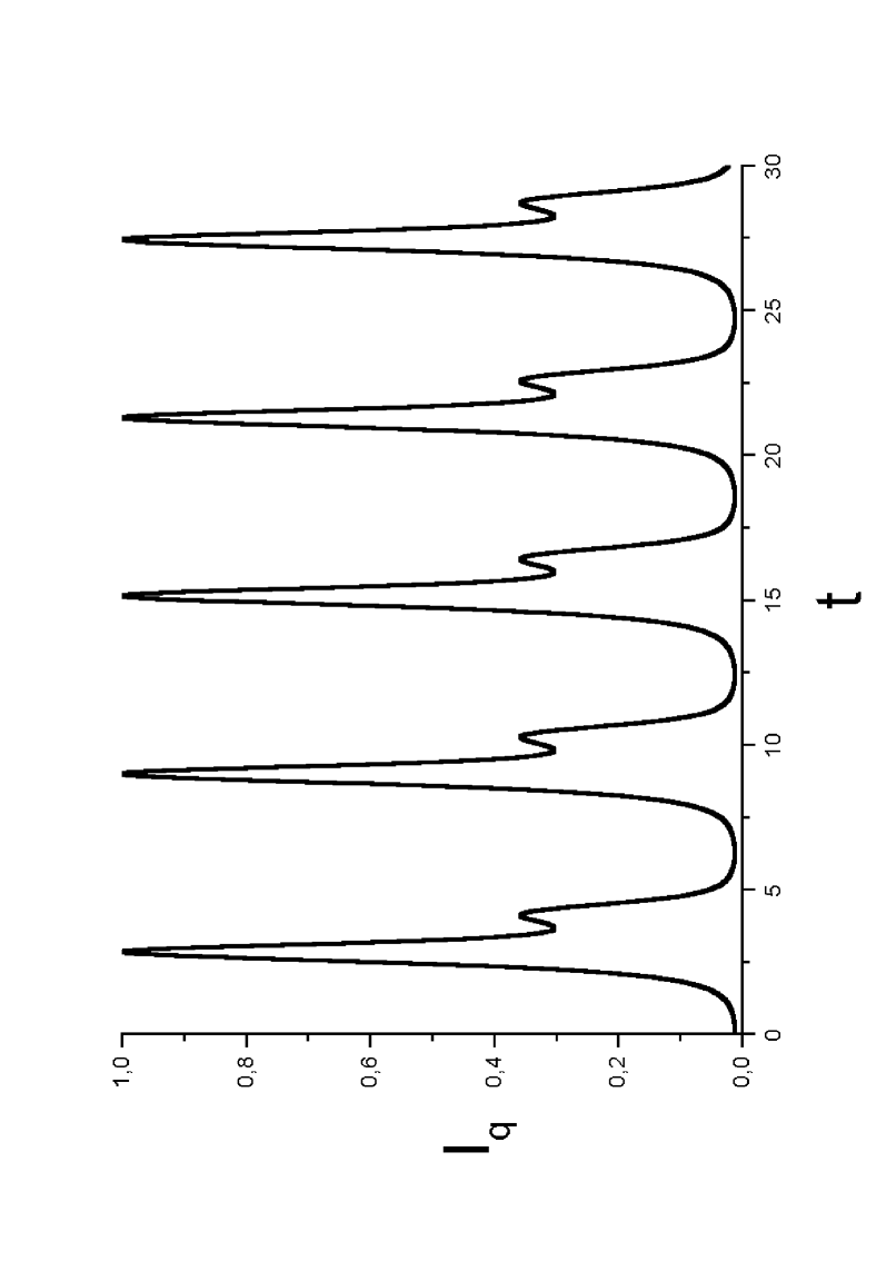
FIG. 1.:

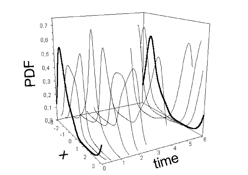
FIG. 2.:

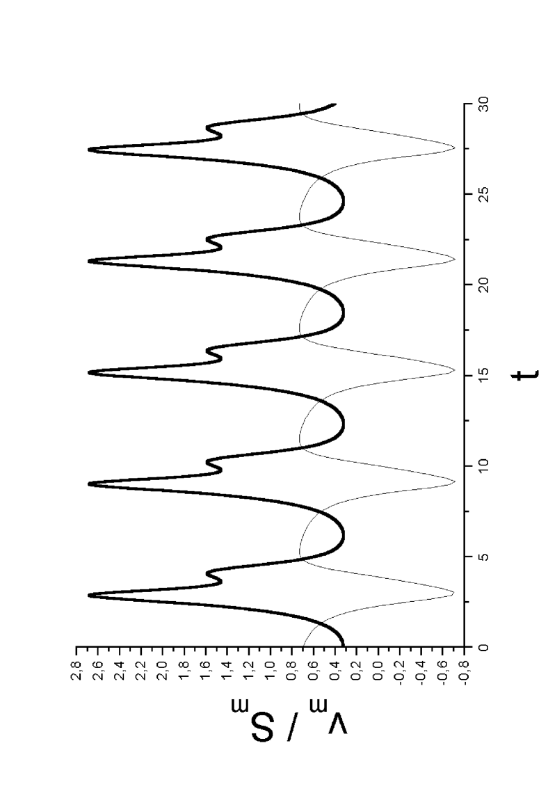
FIG. 3.:

FIG. 4.:

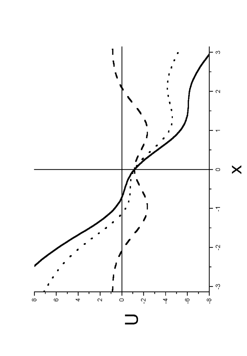
FIG. 5.:

REFERENCES

- [1] G. Nicolis, Introduction to Nonlinear Science, (Cambridge U.P., Cambridge, 1995).
- [2] H.Solari, M.Natiello and G.Mindlin, Nonlinear Dynamics, a two way trip from Physics to Mathematics, (IOP, London, 1996).
- [3] P.Hänggi and P.Riseborough, Am.J.Phys. 45, 347 (1982); see also H. S. Wio, An Introduction to Stochastic Processes and Nonequilibrium Statistical Physics (World Scientific, 1994), ch. 5.
- [4] G. Nicolis, I. Prigogine, Self-Organization in Nonequilibrium Systems, (Wiley, N.Y., 1977); G. Nicolis, Rep. Prog. Phys. 49, 873 (1986); G. Nicolis, Physics of Far-from-Equilibrium Systems and Self-Organization, in The New Physics, P.Davis, Ed. (Cambridge U.P., Cambridge, 1989).
- [5] P.C. Cross and P. Hohenberg, Rev.Mod.Phys. 65, 851 (1993).
- [6] W. Horsthemke and R. Lefever, Noise-Induced Transitions: Theory and Applications in Physics, Chemistry and Biology (Springer-Verlag, Berlin, 1984).
- [7] C. Meunier and A. D. Verga, J. Stat. Phys. 50, 345 (1988); H. Zeghlache, P. Mandel, and C. Van den Broeck, Phys. Rev. A 40, 286 (1989); R. C. Buceta and E. Tirapegui, in Instabilities and Nonequilibrium Structures III, edited by E. Tirapegui and W. Zeller (Kluwer, Dordrecht, 1991), p.171.
- [8] L. Gammaitoni, P. Hänggi, P. Jung, and F. Marchesoni, Rev. Mod. Phys. 70, 223 (1998).
- [9] H. S. Wio, Phys. Rev. E 54, R3075 (1996); F. Castelpoggi and H. S. Wio, Europhys. Lett. 38, 91 (1997); B. Von Haeften, R. Deza, and H. S. Wio, Phys. Rev. Lett. 84, 404 (2000); S. Bouzat and H.S. Wio, Phys. Rev. E 59, 5142 (1999); Horacio S. Wio, B. Von Haeften and S. Bouzat, Proc. 21st STATPHYS, Physica A 306C 140-156 (2002).
- [10] N. V. Agudov, Phys. Rev. E 57, 2618 (1998).
- [11] J. García-Ojalvo and J. M. Sancho, Noise in Spatially Extended Systems, (Springer-Verlag, Berlin, 1999).
- [12] C. Van den Broeck, J. M. R. Parrondo, and R. Toral, Phys. Rev. Lett. 73 (1994); C. Van den Broeck, J. M. R. Parrondo, R. Toral, and R. Kawai, Phys. Rev. E 55, 4084 (1997); S. Mangioni, R. Deza, H. S. Wio and R. Toral, Phys. Rev. Lett. 79, 2389 (1997); S. Mangioni, R. Deza, R. Toral and H. S. Wio, Phys. Rev. E 61, 223 (2000).
- [13] P. Reimann, R. Kawai, C. Van den Broeck and P. Hänggi, Europhys. Lett. 45, 545 (1999).
- [14] S. Mangioni, R. Deza, and H. S. Wio, Phys. Rev. E 63, 041115 (2001); H.S. Wio, S. Mangioni and R. Deza, Physica D 168-169, 184-192 (2002).
- [15] P. Reimann, C. Van den Broeck and R. Kawai, Phys. Rev. E 60, 6402 (1999).
- [16] Y. Kuramoto, Chemical Oscillations, Waves, and Turbulence, (Springer, Berlin, 1984).
- [17] M. A. Fuentes, M. N. Kuperman, H. S. Wio, Physica A 272 574-591 (1999).
- [18] S. Kullback, Information Theory and Statistics, (Wiley, New York, 1959).
- [19] C. Tsallis, J. Stat. Phys. 52 (1988) 479; E.M.F. Curado, C. Tsallis, J. Phys. A 24 (1991) L69; E.M.F. Curado, C. Tsallis, J. Phys. A 24 (1991) 3187; E.M.F. Curado, C. Tsallis, J. Phys. A 25 (1992) 1019.
- [20] See for instance references [1, 2] and also A.C.Newell, The dynamics and analysis of patterns, in Complex Systems, Ed.D.Stein (Addison–Wesley, 1989); A.S. Mikhailov, Foundations of Synergetics I, II, (Springer–Verlag, 1990).
- [21] A. Zaikin and J. Kurths, Chaos 11, 570 (2001)
- [22] H. Sakaguchi, Stochastic synchronization in globally coupled phase oscillators, cond.mat/0210056.