Subgap noise of a superconductor-normal-metal tunnel interface

Abstract

It is well established that the subgap conductivity through a normal-metal-insulator-superconductor (NIS) tunnel junction is strongly affected by interference of electron waves scattered by impurities. In this paper we investigate how the same phenomenon affects the low frequency current noise, $S$, for voltages $V$ and temperatures $T$ much smaller than the superconducting gap. If the normal metal is at equilibrium we find that the simple relation $S(V,T)=4e\,{\rm coth}(eV/T)I(V,T)$ holds quite generally even for non-linear $I$-$V$ characteristics. Only when the normal metal is out of equilibrium, noise and current become independent. Their ratio, the Fano factor, depends then on the details of the layout.

I Introduction

Recently, a great progress has been achieved in the theoretical understanding of current fluctuations in mesoscopic normal-metal superconductor (N-S) hybrid systems.Buttiker ; NazarovBook ; RecentPRLS This progress has been boosted by the development of simple techniques to calculate the full counting statistics of quantum charge transfer.Levitov00 ; NazarovFCS00 ; MuzKhm In particular, the current fluctuations in a diffusive wire in good contact with a superconductor have been calculated taking into account the proximity effect for any voltage and temperature below the gap. BelzigNazarovPRL2001 With proximity effect we mean here the presence of a space dependent coherent propagation in the normal metal of electrons originating from the superconductor. The opposite limit of a tunnel junction between a diffusive metal and a superconductor has been less investigated, partially because only very recently it has become possible to measure current noise in tunnel junctions.CEArecent Theoretically, current noise in a NIS junction has been considered by Khlus long ago,Khlus but neglecting proximity effect. Later, de Jong and Beenakker included the proximity effect at vanishing temperature and voltage.JongBennaker The effect of a finite voltage was studied very recently using a numerical approach.numeric More complicated structures with several tunnel barriers have also been considered. In some limits these can be reduced to a single dominating NIS junction with a complex normal region.BeamSplitter ; Samuelssonn Actually, one may expect that the noise at finite voltage and temperature (of the order of the Thouless energy $E_{th}$) depends on the spatial layout when a tunneling barrier is present,NazarovPRL94 but this has not been investigated so far on general grounds.

As a matter of fact, it has been shown by one of the authors and Nazarov in Ref. HN94, , that the subgap Andreev tunnel current is strongly affected by the coherent scattering of electrons by impurities near the junction region. Two electrons originating from the superconductor with a difference in energy of $\varepsilon$ can propagate on a length scale of the order of $\xi_{\varepsilon}=\sqrt{D/\varepsilon}$ before dephasing ($D$ being the diffusion coefficient and we set $\hbar$ and $k_{B}=1$ throughout the paper). If the relevant energy scale of the problem, i.e. the voltage bias $V$ multiplied by the electron charge $e$ and the temperature $T$ are sufficiently small, the resulting coherence length $\xi_{corr}=\sqrt{D/{\rm max}\{eV,T\}}$ is much larger than the mean free path $l$. Thus at low temperatures and voltages the electron pairs are able to “see” the spatial layout on a length scale given by $\xi_{corr}\gg l$. Since electron pairs attempt many times to jump into the superconductor before leaving the junction region, interference enormously increases the current at low voltage bias and the resulting conductivity depends strongly on the explicit layout.HN94 In this paper we investigate how the same coherent diffusion of pairs of electrons determines the subgap current noise of a NIS tunnel junction.

We find that a generalized Schottky relation holds for voltages and temperatures smaller than the superconducting gap:

$$S(V,T)=4e\,{\rm coth}(eV/T)I(V,T)\/.$$ (1)

Due to the interplay between the proximity effect and the presence of the barrier the current voltage characteristics is both non-universal and non-linear. However, according to Eq. (1), the ratio $F=S/(2eI)=2{\rm coth}(eV/T)$, known as Fano factor, is universal as long as the electron distribution on the normal metal is at equilibrium. In particular, for $T\ll eV$ the Fano factor is 2, indicating that the elementary charge transfer is achieved by Cooper pairs.

If the normal metal is driven out of equilibrium, within our formalism $F$ can be calculated once the geometry is known. One finds then that the noise and the current remain both independent of each other and strongly dependent on the geometry. We discuss a realistic example (cf. Ref. fil, ) where we predict strong deviations from Eq. (1).

The paper is organized as follows. In Section II we set up the main equations and obtain the result given in Eq. (1). In Section III we discuss the case when the normal metallic reservoirs are out of equilibrium. In this case Eq. (1) does not hold and to obtain the Fano factor the diffusive nature of transport will play an important role. Section IV gives our conclusions.

II Tunnelling Hamiltonian approach

Let us consider a normal metallic reservoir connected through a tunnel junction to a superconductor. This problem can be treated conveniently by perturbation theory in the tunnelling amplitude with the standard model Hamiltonian $H=H_{S}+H_{N}+H_{T}$. Here $H_{N}$ and $H_{S}$ describe the disordered normal metal and superconductor:

$$H_{N} = \sum_{{\bf k}\sigma}\xi_{\bf k}c^{\dagger}_{{\bf k}\sigma}c^{\vphantom{{\dagger}}}_{{\bf k}\sigma}\ ,$$ (2)

$$H_{S} = \sum_{{\bf q}\sigma}\zeta_{\bf k}d^{{\dagger}}_{{\bf q}\sigma}d^{\vphantom{{\dagger}}}_{{\bf q}\sigma}+\sum_{{\bf q}}[\Delta d^{\dagger}_{{\bf q}\downarrow}d^{\dagger}_{-{\bf q}\uparrow}+\Delta^{*}d^{\vphantom{{\dagger}}}_{-{\bf q}\uparrow}d^{\vphantom{{\dagger}}}_{{\bf q}\downarrow}]\ ,$$ (3)

$\Delta$ is the superconducting order paramenter, $c_{{\bf k}\sigma}$ and $d_{{\bf q}\sigma}$ are destruction operators for the electrons on the normal and superconducting side, respectively. With ${\bf k}$ and ${\bf q}$ we indicate the eigenstates of the disordered Hamiltonian with eigenvalues $\xi_{\bf k}$ and $\zeta_{\bf q}$, ${\bf q}$ and $-{\bf q}$ indicate time reversed states. The index $\sigma$ stands for the spin projection eigenvalue. The tunnelling part of the Hamiltonian reads:

$$H_{T}=\sum_{{\bf k},{\bf q},\sigma}[t_{{\bf k},{\bf q}}c^{\dagger}_{{\bf k}\sigma}d^{\vphantom{{\dagger}}}_{{\bf q}\sigma}+t^{*}_{{\bf k},{\bf q}}d^{\dagger}_{{\bf q}\sigma}c^{\vphantom{{\dagger}}}_{{\bf k}\sigma}]\,,$$ (4)

where $t_{{\bf k}{\bf q}}=\int d{\bf r}d{\bf r}^{\prime}t({\bf r},{\bf r}^{\prime})\psi_{\bf k}({\bf r})\psi_{\bf q}^{*}({\bf r}^{\prime})$, and $t({\bf r},{\bf r}^{\prime})$ is the quantum amplitude for tunnelling from point ${\bf r}$ of the normal side to point ${\bf r}^{\prime}$ of the superconducting one. All the information on the disorder is in the eigenfunctions $\psi_{{\bf k}/{\bf q}}$. The difference of potential $V$ between the two electrodes can be taken into account by the standard gauge transformation $\xi_{\bf k}\rightarrow\xi_{\bf k}-eV$.

We are concerned only with sub-gap properties: $eV,T\ll\Delta$. No single particle states are available in the superconductor for times longer than $1/\Delta$. Thus the low frequency noise ($\omega\ll\Delta$) will be determined only by tunneling of pairs. Single particle thermal excitations in the superconductor are exponentially suppressed and are thus neglected. To calculate the quantum amplitude for transferring one Cooper pair to the normal metal we proceed as in Ref. HN94, . This gives:

$$A_{{\bf k}{\bf k}^{\prime}}=\sum_{{\bf p}}t^{*}_{{\bf k}{\bf p}}t^{*}_{{\bf k}^{\prime}-{\bf p}}u_{\bf p}v_{\bf p}\left\{{1\over\xi_{\bf k}-E_{\bf p}}+{1\over\xi_{{\bf k}^{\prime}}-E_{\bf p}}\right\}\,,$$ (5)

where ${\bf k}$ and ${\bf k}^{\prime}$ indicate the final electron states (assumed empty), $v^{2}_{\bf p}=1-u^{2}_{{\bf p}}=(1-\zeta_{\bf p}/E_{\bf p})/2$ are the BCS coherence factors, and $E_{\bf p}=(\zeta_{\bf p}^{2}+\Delta^{2})^{1/2}$ is the superconducting spectrum.

The function $A$ gives the amplitude for the only possible elementary process at low energies. It is thus convenient to write an effective tunnelling Hamiltonian in terms of these processes,

$$H^{eff}=H_{N}+J+J^{\dagger}\quad{\rm with}\quad J=\sum_{{\bf k}{\bf k}^{\prime}}A_{{\bf k}{\bf k}^{\prime}}c^{\dagger}_{{\bf k}\uparrow}c^{\dagger}_{{\bf k}^{\prime}\downarrow}b_{o}\,,$$ (6)

where $b_{o}=(2/N_{S})\sum_{\bf q}\phi_{\bf q}d_{{\bf q}\uparrow}d_{-{\bf q}\downarrow}$ is the destruction operator for a Cooper pair in the condensate, $\phi_{\bf q}=v_{\bf q}/u_{\bf q}$ is the pair wavefunction and $N_{S}$ is the number of fermions on the superconducting side. Note that $b_{o}$ is not a true bosonic operator, since Cooper pairs overlap.PistolesiStrinati In practice, since the superconductor is in the coherent phase, the averages involving $b_{o}$ are trivial to perform (we neglect collective-modes excitations, which are at higher energy): $\langle b_{o}\rangle=\langle b^{\dagger}_{o}\rangle=\langle b_{o}^{\dagger}b_{o}\rangle=1$. A similar Hamiltonian, but with a constant amplitude, has been considered by many authors to study the influence of collective modes on Andreev reflection from a phenomenological point of view.Wen ; Falci Here we found its form from the BCS microscopic model, the resulting $H^{eff}$ is thus equivalent to the starting one (4) at low energies.

The current operator can be obtained as usual by the time derivative of $N=\sum_{{\bf q}\sigma}c^{\dagger}_{{\bf k}\sigma}c^{\vphantom{{\dagger}}}_{{\bf k}\sigma}$:

$$I(t)=e\,\frac{dN}{dt}=ei[H^{eff}_{T},N]=-2ei[J(t)-J^{\dagger}(t)]\ .$$ (7)

We have now all the elements to calculate by perturbative expansion in the new coupling $A$ ($\sim t^{2}$) the quantum average of the current, $\langle I\rangle$, and of the current-noise-spectral density:

$$S(\omega=0)=\int_{-\infty}^{+\infty}dt[\langle[I(t),I(0)]_{+}\rangle-2\langle I(t)\rangle\langle I(0)\rangle]\,.$$ (8)

Writing the evolution operator in the interaction representation $U(t)=T\exp\{-i\int_{-\infty}^{t}dt^{\prime}[J_{o}(t^{\prime})+J_{o}^{\dagger}(t^{\prime})]\}$, where $J_{o}(t)$ evolves according to $H_{N}$, one can readily expand in $A$ and obtain in lowest order the following expression for $I$ and $S$:

$$I(t=0) = 2e[N_{\leftarrow}-N_{\rightarrow}]$$ (9)

$$S(\omega=0) = 8e^{2}[N_{\leftarrow}+N_{\rightarrow}]$$ (10)

where

$$N_{\rightarrow}=\int_{-\infty}^{\infty}\!\!\!\!\!\!\!\!dt^{\prime}\langle J_{o}(0)J_{o}^{\dagger}(t^{\prime})\rangle\quad,\quad N_{\leftarrow}=\int_{-\infty}^{\infty}\!\!\!\!\!\!\!\!dt^{\prime}\langle J_{o}^{\dagger}(t^{\prime})J_{o}(0)\rangle\,.$$

This result depends only on the fact that the current can be described as a first order process in the effective tunnelling amplitude $A$. For the tunnelling case Levitov and ReznikovLevitovbipoissonian showed that the full counting statistics is bi-poissonian:

$$\ln\chi(\lambda)=(e^{2ie\lambda}-1)N_{\leftarrow}+(e^{-2ie\lambda}-1)N_{\rightarrow}\,,$$ (11)

where $\chi$ is the generating function. Taking successive derivatives with respect to $i\lambda$ of $\ln\chi$ and setting $\lambda=0$ afterwards one generates current momenta of all orders. It is readily verified that $I=\partial\ln\chi/\partial(i\lambda)$, and $S=2\partial^{2}\ln\chi/\partial(i\lambda)^{2}$ coincide with (9)-(10). Eq. (11) implies that $I$ and $S$ determine the full counting statistics of the problem. The physical picture is simple: the distribution of transmitted Cooper pairs is given by a superposition of two Poissonians for tunnelling from left to right and from right to left.

If the metallic side is at the thermodynamic equilibrium the full dependence of noise on voltage and temperature is given on general grounds by (1). This relation can be proven by evaluating (9) and (10) using the basis of eigenstates $|n\rangle$ of $H_{N}$ with eigenvalues $E_{n}$. One can actually write $I=2eC_{-}$ and $S=8e^{2}C_{+}$ with

$$C_{\pm} = \sum_{n\,m}\int_{-\infty}^{+\infty}\!\!\!\!\!\!\!\!\!dt\,e^{2ieVt}{e^{-E_{n}/T}\over{\cal Z}}\times$$ (12)

$$\left(|J_{mn}|^{2}e^{i\omega_{nm}t}\pm|J_{nm}|^{2}e^{-i\omega_{nm}t}\right)$$

where $\omega_{nm}=E_{n}-E_{m}$, ${\cal Z}=\sum_{n}e^{-E_{n}/T}$ is the partition function and $J_{nm}=\langle n|J|m\rangle$. By simple manipulations of Eq. (12) one obtains

$$C_{\pm}=2\pi\left(1\pm e^{2eV/T}\right)\sum_{n\,m}{e^{-E_{n}/T}\over{\cal Z}}|J_{nm}|^{2}\delta(2eV-\omega_{nm})\,.$$ (13)

From Eq. (13) the relation (1) follows directly. Note that the proof is valid for any system at thermal equilibrium, interactions in the normal metal do not spoil the result. For a generic tunnelling system the relation between noise and current was shown by Sukhorukov and LossSukoLoss and discussed recently by Levitov.LevitovErice

One thus finds that non-linear dependence on the voltage and temperature of the current will be found exactly in the low frequency noise with a universal Fano factor of $F=S/(Ie)=2\coth(eV/T)$. In the completely coherent case ($A$ independent of energy, i.e. $eV\ll E_{th}$) the same equation has been proved in Ref. Martin, . In this paper we extend its validity to arbitrary ratio $eV/E_{th}$ provided $eV\ll\Delta$. Few comments are in order. Eq. (1) can be regarded as a generalization of the fluctuation dissipation theorem, since it holds for any value of the perturbing field $V$.SukoLoss We would point out also that in presence of interactions among electrons the noise was calculated recently in Ref. SLF, with the limitation $eV\ll E_{th}$. We mention that for a normal wire in good contact with the superconductor the situation is much richer and the full energy dependence of the Fano factor has been calculatedBelzigNazarovPRL2001 and measured.Jehl ; Prober1 ; Prober2 For this case an analytical expression that links the current to the noise was proposed,Houzet but it does not reproduce the weak energy dependence of the differential Fano factor [cf. Eq. (28) in the following]. Only very recently an analytical solution of the generalized Usadel equation introduced in Ref. BelzigNazarovPRL2001, has been obtained.HouzetPistolesi

In order to emphasize the generality of Eq. (1) let us consider a non-trivial example. In Ref. Gueron, the low-voltage anomalies due to the proximity effect have been detected in a superconducting ring closed on a normal metal through two tunnel junctions as shown in Fig. (1).

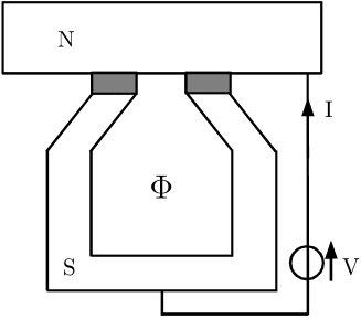
Figure 1: Experimental set up similar to Ref Gueron, . The magnetic flux dependence of the current and noise can be used to measure the doubling of the Fano factor with high accuracy.

Part of the subgap current through this structure is modulated by the external magnetic field. Using Eq. (1) one can predict the following noise dependence on the magnetic flux $\Phi$ through the ring: $S(\Phi)=4e\,{\rm coth}(eV/T)I(\Phi)$. Since the $\Phi$ dependent part is given by the coherent propagation of two electrons between the two junctions any single particle contribution is eliminated from the outset. This experiment could thus be used to test accurately the validity of Eq. (1) and in particular the doubling of the charge at low temperature.

III Out of equilibrium reservoirs in diffusive junctions

When the normal metal is not at equilibrium the simple relation (1) between $S$ and $I$ does not hold any longer, and expressions (9) and (10) have to be evaluated explicitly. We proceed by writing:

$$I = 4\pi e\sum_{{\bf k}{\bf k}^{\prime}}|A_{{\bf k}{\bf k}^{\prime}}|^{2}\delta(\xi_{\bf k}+\xi_{{\bf k}^{\prime}}-2eV)H_{-}(\xi_{\bf k},\xi_{{\bf k}^{\prime}})\,,$$

$$S = 16\pi e^{2}\sum_{{\bf k}{\bf k}^{\prime}}|A_{{\bf k}{\bf k}^{\prime}}|^{2}\delta(\xi_{\bf k}+\xi_{{\bf k}^{\prime}}-2eV)H_{+}(\xi_{\bf k},\xi_{{\bf k}^{\prime}})\,,$$

where:

$$H_{\pm}(\xi,\xi^{\prime})=[1-n(\xi)][1-n(\xi^{\prime})]\pm n(\xi)n(\xi^{\prime})\,,$$ (14)

and $n(\xi_{\bf k})=\langle c^{\dagger}_{{\bf k}\sigma}c^{\vphantom{{\dagger}}}_{{\bf k}\sigma}\rangle$. It is convenient to introduce the relevant energy dependence by defining:

$$A(\varepsilon,eV)=\sum_{{\bf k}{\bf k}^{\prime}}\delta(\varepsilon/2+eV-\xi_{\bf k})\delta(-\varepsilon/2+eV-\xi_{{\bf k}^{\prime}})|A_{{\bf k}{\bf k}^{\prime}}|^{2}.$$

We thus obtain:

$$\left({I\atop S}\right)=2\pi e\!\!\!\int_{-\infty}^{\infty}\!\!\!\!\!\!d\varepsilon A(\varepsilon,eV)\left({H_{-}({\varepsilon\over 2}+eV,-{\varepsilon\over 2}+eV)\atop 4eH_{+}({\varepsilon\over 2}+eV,-{\varepsilon\over 2}+eV)}\right)\,.$$ (15)

If the normal metal is in thermal equilibrium $n(\xi)$ is the Fermi distribution $f_{F}(\xi)$. In that case $H_{+}$ and $H_{-}$ are related by the simple relation:

$${H_{+}(\varepsilon/2+eV,-\varepsilon/2+eV)\over H_{-}(\varepsilon/2+eV,-\varepsilon/2+eV)}={\rm coth}\left({eV\over T}\right)\ ,$$ (16)

and we recover again Eq. (1). If $n(\xi)\neq f_{F}(\xi)$, Eq. (16) does not hold and $S$ and $I$ become independent. Indeed, the Fano factor ceases to be universal and gives new information on the system. The technique developed so far enables calculation of $F$ also in this case through Eq. (15), however now we need to specify the explicit form of $A(\varepsilon)$. We follow Refs. HN94, to evaluate it:

$$A(\varepsilon,eV)=\int d\zeta d\zeta^{\prime}d\xi d\xi^{\prime}F(\zeta;\xi,\xi^{\prime})F(\zeta^{\prime};\xi,\xi^{\prime})\times$$

$$\Xi(\zeta,\zeta^{\prime};\xi,\xi^{\prime})\delta(\varepsilon/2+eV-\xi)\delta(\varepsilon/2-eV+\xi^{\prime})$$

where $F(\zeta;\xi,\xi^{\prime})=u(\zeta)v(\zeta)\{(\xi+eV-E(\zeta))^{-1}+(\xi^{\prime}+eV-E(\zeta))^{-1}\}$,

$$\Xi[\zeta,\zeta^{\prime},\xi,\xi^{\prime}]=\!\int\!\!d^{3}{\bf r}_{1}\dots d^{3}{\bf r}_{4}\int\!\!d^{3}{\bf r}^{\prime}_{1}\dots d^{3}{\bf r}^{\prime}_{4}\times$$ (17)

$$\langle K_{\xi}({\bf r}_{1},{\bf r}_{3})K_{\xi^{\prime}}({\bf r}_{2},{\bf r}_{4})\rangle_{imp}\langle K_{\zeta}({\bf r}^{\prime}_{2},{\bf r}^{\prime}_{1})K_{\zeta^{\prime}}({\bf r}^{\prime}_{4},{\bf r}^{\prime}_{3})\rangle_{imp}\times$$

$$t^{*}({\bf r}_{1},{\bf r}^{\prime}_{1})t^{*}({\bf r}_{2},{\bf r}^{\prime}_{2})t({\bf r}_{3},{\bf r}^{\prime}_{3})t({\bf r}_{4},{\bf r}^{\prime}_{4})\,.$$

Merely $K_{\xi}({\bf r}_{1},{\bf r}_{2})=\sum_{\bf k}\delta(\xi-\xi_{\bf k})\psi_{\bf k}({\bf r}_{1})\psi^{*}_{\bf k}({\bf r}_{2})$ is the single particle propagator and $\langle\dots\rangle_{imp}$ indicates impurity average. Since the tunnelling is most probable only near the surface of the junctions, we can set ${\bf r}_{i}={\bf r}^{\prime}_{i}$ and restrict them to lie on the surface. The impurity averages can be performed within the usual approximation $k_{F}l\gg 1$ ($k_{F}$ Fermi momentum). The main contribution to Eq. (17) is given by the “Cooperon” diagrams, associated to the coherent propagation of two interfering electrons with small energy difference $\varepsilon$ and small total momentum. The range of the Cooperon propagator is $\xi_{\varepsilon}$, and thus it is much larger than the range of $K_{\xi}({\bf r},{\bf r}^{\prime})$ which is $l$. For this reason among the integrals over $d^{2}{\bf r}$ two dominant terms can be singled out: (a) the term where ${\bf r}_{1}\approx{\bf r}_{2}$ and ${\bf r}_{3}\approx{\bf r}_{4}$ with interference occurring in the normal metal and (b) the term where ${\bf r}_{1}\approx{\bf r}_{3}$ and ${\bf r}_{2}\approx{\bf r}_{4}$ with interference occurring in the superconductor. Since in Ref. HN94, it has been shown that the second term is always smaller than the first by a factor $eV/\Delta$ we consider only case (a). The dominant contribution to $\Xi$ can thus be written as follows: $\Xi[\zeta,\zeta^{\prime};\xi,\xi^{\prime}]\approx\Xi(\xi-\xi^{\prime})$ and

$$\Xi(\varepsilon)={G_{T}^{2}\over 32\pi^{3}e^{4}\nu_{N}{\cal S}^{2}}\int d^{2}{\bf r}_{1}d^{2}{\bf r}_{2}[P_{\varepsilon}({\bf r}_{1},{\bf r}_{2})+P_{-\varepsilon}({\bf r}_{1},{\bf r}_{2})]\,.$$ (18)

Here $G_{T}$ is the conductance in the normal phase, ${\cal S}$ is the surface area of the junction, $\nu_{N}$ is density of states of the normal metal (per spin) and $P_{\varepsilon}({\bf r})$ satisfies the diffusion equation in the normal metal:

$$(-D\nabla_{1}^{2}-i\varepsilon)P_{\varepsilon}({\bf r}_{1},{\bf r}_{2})=\delta^{3}({\bf r}_{1}-{\bf r}_{2})\,.$$ (19)

The integration over $\zeta$ and $\zeta^{\prime}$ for $\xi,\xi^{\prime},eV\ll\Delta$ can be done and gives $\pi^{2}$, we are thus left with an explicit expression for $A(\varepsilon)=\pi^{2}\Xi(\varepsilon)$ which can be calculated if the geometry of the system is known. Given $A$ and $n(\xi)$ the noise and the current can be found explicitly from (15) and (14).

III.1 An explicit example: a wire out of equilibrium

We are now in a position to calculate both current and noise in a non-equilibrium system. Let us consider a realistic example: In Ref. fil, the non-equilibrium electron distribution for a small metallic wire of length $L$ has been measured by using a tunnel junction between the wire (at different positions $x$ along the wire) and a supercondutor (see also inset of Fig. 3 in the following). In that case the quasiparticle current was measured, but the subgap current and noise in the same configuration could also be measured. When $L$ is shorter than the inelastic mean free path the electron distribution along the wire is given by the diffusion equation:fil

$$n(x,\xi)=f_{F}(\xi+eU)[1-x/L]+f_{F}(\xi)x/L$$ (20)

where $U$ is the difference of potential between the two normal reservoirs. This leads to a double discontinuity of the distribution function at $T=0$.

Since the transverse dimension $w$ of the wire is much smaller than $\xi_{corr}$, we can use the one dimensional diffusion equation. Following Ref. Altshuler, we impose the boundary condition on the propagator $P$ corresponding to a good contact with a reservoir. This means that $P_{\varepsilon}(x_{1},x_{2})$ should vanish when $x_{1}=0$ or $L$. In the dimensionless variables $u=x/L$, Eq. (19) becomes

$${d^{2}P\over du^{2}_{1}}(u_{1},u_{2})+i{\varepsilon\over E_{th}^{W}}P(u_{1},u_{2})=-{L\over w^{2}D}\delta(u_{1}-u_{2})$$ (21)

with the boundary conditions $P(0,u_{2})=P(1,u_{2})=0$ and where $E_{th}^{W}=D/L^{2}$ is the Thouless energy of the wire. The solution can be written as a sum of a special solution of the complete equation plus a linear combination of the two linearly independent solutions of the homogeneous equation. The coefficients of this combination can be chosen in such a way as to fulfill boundary conditions. The solution reads:

$$P(u_{1},u_{2})={L\over 2Dw^{2}z}\left[e^{-z|u_{1}-u_{2}|}\phantom{a^{a}\over b^{a}}\right.$$

$$\left.-{e^{z(u_{1}+u_{2})}+e^{z(u_{1}+u_{2}-2)}-e^{z(u_{1}-u_{2})}-e^{-z(u_{1}-u_{2})}\over e^{2z}-1}\right]\,,$$

where, for $\varepsilon>0$ , $z=\sqrt{\varepsilon/E_{th}^{W}}e^{-i\pi/4}$. Inserting Eq. (LABEL:soluP) into Eq. (18) and assuming that the size of the junction is small, we have

$$\Xi(\varepsilon)={G_{T}^{2}L\over 16\pi^{3}e^{4}\nu_{N}Dw^{2}}\,\phi(\varepsilon)\,,$$ (23)

where

$$\phi(\varepsilon)={\rm Re}\left[{\sinh(zu_{0})\sinh(z(1-u_{0}))\over z\sinh(z)}\right]\,,$$ (24)

and $u_{0}$ indicates the position of the junction along the wire. Introducing the conductance of the wire $G_{W}=2w^{2}e^{2}D\nu_{N}/L$ and using Eq. (15), the expression for the current simplifies to

$$I={G_{T}^{2}\over 4eG_{W}}\int\!\!d\varepsilon\,\phi(\varepsilon)H_{-}(\varepsilon/2-eV,-\varepsilon/2-eV)\,.$$ (25)

The noise obeys an identical expression with $H_{-}\rightarrow 4eH_{+}$. Note that in the limit of an infinite wire the function $\phi(\varepsilon)\sim 1/\sqrt{\varepsilon}$ diverges at low energy, as expected for one dimensional diffusion. Substituting Eq. (14) with Eq. (20) into Eq. (25) one obtains current and noise for any temperature, voltage, and position along the wire. Let us consider for simplicity one specific case: zero temperature and voltage $0\leq V\leq U/2$. It is not difficult to show that in this case

$$I={G_{T}^{2}\over 2eG_{W}}\phi_{-}\,,\quad{\rm and}\quad S=2{G_{T}^{2}\over G_{W}}\phi_{+}$$ (26)

with

$$\phi_{\pm}=(1-u_{0})\int_{2eV}^{2e(U-V)}\!\!\!\!\!\!\!\!\!\!\!\!\!\!\!\!\!\!\phi(\varepsilon)d\varepsilon+[(1-u_{0})^{2}\pm u_{0}^{2}]\int_{0}^{2eV}\!\!\!\!\!\!\!\!\ \phi(\varepsilon)d\varepsilon\,.$$ (27)

Differentiating with respect to $V$ Eqs. (26) gives the differential Fano factor

$${\cal F}(eV)\equiv{(dS/dV)\over(2e\,dI/dV)}\,.$$ (28)

In our case ${\cal F}$ is given by the following expression

$${\cal F}(eV)=2{(1-u_{0})\phi(2eU-2eV)-u_{0}\,(2u_{0}-1)\phi(2eV)\over(1-u_{0})\phi(2eU-2eV)+u_{0}\phi(2eV)}\,.$$ (29)

Note that normally the Fano factor is positive since it corresponds to the (positive) current noise divided by the absolute value of the current. The differential Fano factor is then usually defined in such a way that a factor sign$(I)$ is implicit in the definition. This makes it usually positive, since current and the noise are supposed to increase with the voltage bias. But in our case the wire is off-equilibrium, thus the voltage $V$ has not the usual meaning of bias voltage between two systems at local equilibrium. Along the wire it is not even possible to define a chemical potential, since fermions are not at equilibrium. Thus the concept of difference of potential between the superconductor and the wire at the position of the contact is ill-defined. The potential $V$ is nevertheless well defined and can be used to study the evolution of the conductance or of the differential noise. Clearly the sign of the current needs not be the same as that of V. For this reason we use the definition (28) as it is, without changing the sign according to the direction of the current. This allows a more simple representation in Fig. 2. One should keep in mind that the change of sign has no special meaning in this case, since increasing the voltage bias $V$ can well decrease the current and the noise at through the SIN junction.

Let us discuss briefly some simple limiting cases of Eq. (29). For $u_{0}=0$ and $1$, when the junction is at the extremities of the wire, Eq. (29) gives ${\cal F}=\pm 2$. This is expected from Eq. (1) since in this case the normal metal is actually at equilibrium. The sign change is simply due to fact that for $x=0$ the potential of the wire $U$ is greater than the potential of the superconducting point $V$, while for $x=L$ the situation is reversed. For $0<u_{0}<1$, ${\cal F}$ is in general different from 2. An interesting point is the middle of the wire $u_{0}=1/2$. In this case we have:

$${\cal F}(eV,u_{0}=1/2)=2{\phi(2eU-2eV)\over\phi(2eV)+\phi(2eU-2eV)}\,.$$ (30)

For $V=U/2$ we then obtain ${\cal F}=1$ exactly for any form of $\phi(\varepsilon)$, while for $V=0$ ${\cal F}$ should become very small on general grounds, since we have seen that for $\varepsilon\rightarrow 0$ the function $\phi(\varepsilon)$ is expected to diverge in the infinite system.

Figure 2: Differential Fano factor ${\cal F}$ as a function of $V/U$. Different curves represent different values of $u_{0}$ going from 0 to 1 in step of 0.1 starting from the top. Departure from the value 2 or -2 is due to the energy dependence of the tunnelling matrix element.

For arbitrary values of $u_{0}$ one can see a crossover between these limiting behaviors. We report in Fig. 2 the results predicted by Eq. (29) for $U=200E_{th}^{W}$ which is a typical value for experiments. We would like to emphasize that the whole energy dependence seen in this plot is due to interference of electronic waves, since it stems from the $\varepsilon$-dependence of $\phi(\varepsilon)$.

III.2 Comparison with circuit theory approach

It can be useful to obtain current and noise with an alternative technique, often called circuit theory, developed by Nazarov and coworkers. NazarovFCS00 ; RecentPRLS ; BelzigNazarovPRL2001 ; Belzig The assumptions behind circuit theory are the same as the ones that have been used to arrive to Eq. (29), but its scope is much larger, since it can be applied for arbitrary transparency of the interface. On the other hand its implementation is often numerical and can become extremely cumbersome in higher dimension. In the case at hand of a wire the problem can be solved rather easily and it is worth to compare the results of the two techniques.

We follow Belzig and NazarovBelzigNazarovPRL2001 in modelling the wire within semiclassical Green’s function technique. The wire is describled by $N$ nodes, each node represents a part of the wire small enough such that the inhomogeneities inside can be neglected. Each node is thus completely described by one Usadel 4x4 matrix $\check{\cal G}$ in the Nambu$(\,\hat{}\,)$-Keldysh$(\,\bar{}\,)$ space with the condition $\check{\cal G}^{2}=1$. The nodes are connected by tunnel junctions with conductance $g_{T}=(N+1)G_{W}$ in such a way that the total conductance of the wire is $G_{W}$. Kuprianov-LukichevKL boundary conditions plus the decoherence term in Usadel equation give the following condition to be satisfied at each node $i$

$$[\check{\cal A}_{i},\check{\cal G}_{i}]=0$$ (31)

where

$$\check{\cal A}_{i}=g_{T}\,(\check{\cal G}_{i+1}+\check{\cal G}_{i-1})-2i{\varepsilon\over N\,E_{th}^{W}}\check{\tau}_{3},$$ (32)

$\check{\tau}_{3}=\hat{\tau}_{3}\otimes\bar{1}$, and $\bar{\sigma}_{i},\hat{\tau}_{j(i,j=1,2,3)}$ are Pauli matrices ($\bar{\sigma}$ will appear in the following). The boundary conditions at the two extremities are given by the bulk solution for the normal metal at equilibrium: $\check{\cal G}_{N}^{0}=\hat{\tau}_{3}\otimes\bar{\sigma}_{3}+(f_{T0}+f_{L0}\hat{\tau}_{3})\otimes(\bar{\sigma}_{1}+i\bar{\sigma}_{2})$ with $f_{L0}=1-f_{+}-f_{-}$, $f_{T0}=f_{-}-f_{+}$, $f_{\pm}(\varepsilon)=f(\varepsilon\pm eU_{L/R})$, $f$ is the Fermi function at temperature $T$, and $U_{L/R}$ is the voltage bias at (L) $x=0$ and at (R) $x=L$. Eq. (31) has a simple analytical solution: $\check{\cal G}=\check{\cal A}_{i}/\sqrt{\check{\cal A}_{i}^{2}}$, and the full set of equations can be solved by iteration leading to an explicit numerical value for $\check{\cal G}_{i}$ at each node.

This describes a normal wire in good contact with two normal reservoirs kept at some voltage bias $U_{L}$ and $U_{R}$ with respect to (an arbitrary) ground. We add now the superconducting tunnel contact with conductance $G_{T}$ at node $s$, with $1\leq s\leq N$. Since it is easier technically to keep the superconductor at zero voltage with respect to ground, we set $U_{L}=U-V$ and $U_{R}=-V$. The tunnel contact with the superconductor modifies the conditions (32) for node $s$ in the following way:

$$\check{\cal A}_{s}=g_{T}\,(\check{\cal G}_{s+1}+\check{\cal G}_{s-1})+G_{T}\,\check{\cal G}_{S}(\chi)-2i{\varepsilon\over N\,E_{th}^{W}}\check{\tau}_{3}\,.$$ (33)

(Since $G_{T}\ll g_{T}$ we can neglect corrections to the Thouless energy due to the presence of the superconducting reservoir.) The Green’s function $\check{\cal G}_{S}(\chi)$ is the superconducting bulk solution of the semiclassical equations, modified by the introduction of a counting field $\chi$. This means that $\check{\cal G}_{S}(\chi)=e^{-\frac{i}{2}\chi\check{\tau}_{K}}\,\check{\cal G}_{S}^{0}\,e^{\frac{i}{2}\chi\check{\tau}_{K}}$ with $\check{\cal G}_{S}^{0}=\hat{\tau}_{2}\otimes\bar{1}$ (since all energies are smaller than the superconducting gap) and $\check{\tau}_{K}=\hat{\tau}_{3}\otimes\bar{\sigma}_{1}$. The circuit is shown in the inset of Fig. 3. Once the solution to the system of equations has been found it is possible to obtain the current, the noise, and, in principle, all higher cumulants of the current flowing through the SIN junction by evaluating

$$J(\chi)=-{G_{T}\over 8e}\int d\varepsilon\,{\rm Tr}\left\{\check{\tau}_{K}[\check{\cal G}_{s},\check{\cal G}_{S}]\right\}\,.$$ (34)

The current is given by $J(\chi=0)$ while the noise is proportional to its first derivative with respect to $\chi$: $S=-2ie\partial J/\partial\chi$. Numerically one can obtain both at the same time, since for very small $\chi$ the first is proportional to the real part of $J(\chi)$ while the second to its imaginary part.

We have thus found numerically the current and the noise for $U=200E_{th}^{W}$ and different values of $V$. The numerical results presented refers to 18 nodes. The tunnel conductance $G_{T}$ was chosen much smaller than $g_{T}$ ($g_{T}/G_{T}\sim 10^{3}$) and we have verified that both current and noise scale with $G_{T}^{2}$ as predicted by Eq. (26).

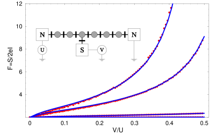
Figure 3: Fano factor as a function of $V/U$ for $x/L=9/18,$ 8/18, 4/18, and 1/18, from top to bottom. Full lines are obtained with Eq. (26). The dots indicate the result obtained with circuit theory. The inset shows the circuit used in the calculation.

In Fig. 3 we show the Fano factor as a function of $V/U$ ($U=200E_{th}^{W}$, $V<U/2$) for different value of $s$, the node in contact with the superconductor. The agreement between the two approaches is rather good.

A strong effect of the non equilibrium distribution is the divergence of the Fano factor for certain values of $V$ or $u_{0}$, while at equilibrium and at zero temperature Eq. (1) predicts invariably $F=2$. In the case shown in Fig. 3 the divergence appears for $x=L/2$ and $V=U/2$. This divergence can be easily understood, since at these values of the bias and position along the wire the current vanishes with $N_{\rightarrow}=N_{\leftarrow}\neq 0$ [cf. Eq. (9)] such that the resulting $S$ is non vanishing [cf. Eq. (10)]. Even if this is a large effect it is mainly due to the fact that the system is out of equilibrium, and it is thus not a direct signature of the importance of the interference in the noise. Interference appears instead directly in the differential Fano factor $\cal F$.

A more stringent test on the validity of both approaches is thus to compare ${\cal F}(eV)$. Our rather simplified numerical approach to the circuit theory allows to extract the derivatives of $S$ and $I$ with a limited accuracy. Nevertheless the agreement of the analytical expression (29) and the numerical results shown in Fig. 4 is reasonable, and it remains within the numerical error of the circuit theory calculation.

There are actually other reasons for possible discrepancies between the two approaches. In the analytical calculation we have not taken into account that the Fermi distribution changes along the wire due to the electric field, while this effect is included in the circuit theory approach.

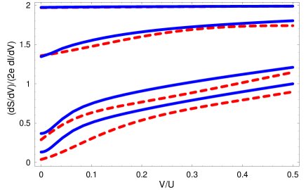
Figure 4: Comparison of the differential Fano factor $\cal F$ given by Eq. (29) (full lines) and by the numerical circuit theory simulation (dashed lines). The four dashed curves are obtained for $U=200E_{th}^{W}$ and $u_{0}=1/18$, 4/18, 8/18, and 9/18 ($N=18$).

IV Conclusions

In conclusion we have found a general expression that links the subgap noise and the current in a NIS junction. The interference of electron pairs leads to a non-linear dependence of current and noise on voltage, but their ratio is fixed by Eq. (1) as long as the electrons in the normal metal are in equilibrium. Out of equilibrium, the Fano factor becomes non universal and we have computed it in a feasible experiment. In particular we have studied the differential Fano factor, which is a direct measure of the importance of interference of electronic waves. The validity of Eq. (1) is quite general, it does not depend on the interactions in the normal metal, for instance. Thus detecting a departure from this prediction can be a strong experimental indication that the normal metal is out of equilibrium.

From the technical point of view we have verified that the tunnelling approach agrees with the circuit theory approach. Both stem from the semiclassical theory of current fluctuations, but it is clear that the tunnelling calculation is often much simpler than solving the full Usadel equations. It is thus useful to verify that it can give reliable quantitative prediction for both the current and the noise in a specific example.

Let us briefly discuss a possible experimental test of Eq. (1). Due to the large barriers induced by oxides, experiments on shot noise in tunnel junctions are not as developed as they are for the transparent junctions. The only data available at this momentCEArecent appear to agree reasonably well with our prediction. Indeed, current and noise both show a strong non-linear behavior, but their ratio follows the simple relation (1).

We are indebted to M. Houzet for useful discussions. We acknowledge financial support from CNRS/ATIP-JC 2002 and Institut Universitaire de France.

References

- (1) For a recent review see Y.M. Blanter and M. Büttiker, Phys. Rep. 336, 1 (2000).
- (2) Quantum noise in mesoscopic systems, edited by Y. V. Nazarov, Kluwer, Dordrecht (2003).
- (3) W. Belzig and Y.V. Nazarov, Phys. Rev. Lett. 87, 197006 (2001); Y. V. Nazarov and D.A. Bagrets, ibid 88, 196801 (2002).
- (4) L.S. Levitov, H.W. Lee, and G.B Levitov, J. Math. Phys. 37, 4845 (1996).
- (5) Y. V. Nazarov, Ann. Phys. (Leipzig) 8, SI-193 (1999).
- (6) B.A. Muzykantskii and D.E. Khmelnitskii, Phy. Rev. B 50, 3982 (1994).
- (7) W. Belzig and Y.V. Nazarov, Phys. Rev. Lett. 87, 067006 (2001).
- (8) F. Lefloch, C. Hoffmann, M. Sanquer, and D. Quirion, Phys. Rev. Lett. 90, 067002 (2003).
- (9) V.A. Khlus, Sov. Phys. JETP 66, 1243 (1987).
- (10) M.J.M. de Jong and C.W.J. Beenakker, Phys. Rev. B 49, 16070 (1994).
- (11) M.P.V. Stenberg and T.T. Heikkilä, Phys. Rev. B, 66, 144504 (2002).
- (12) J. Börlin, W. Belzig, and C. Bruder, Phys. Rev. Lett. 88 197001 (2002); P. Samuelsson and M. Büttiker, ibid., 89, 046601 (2002).
- (13) P. Samuelsson, Phys. Rev. B 67, 054508 (2003).
- (14) Y.V. Nazarov, Phys. Rev. Lett. 73, 134 (1994).
- (15) F.W.J. Hekking and Y.V. Nazarov, Phys. Rev. Lett. 71, 1625-1628 (1993) and Phys. Rev. B 49 6847 (1994).
- (16) H. Pothier, S. Guéron, N.O. Birge, D. Esteve, M.H. Devoret, Z. Phys. B 104, 178, (1997).
- (17) F. Pistolesi and G.C. Strinati, Phys. Rev. B 53, 15168 (1996).
- (18) Y.B. Kim and X.-G. Wen, Phys. Rev. B 48, 6319 (1993).
- (19) G. Falci, R. Fazio, A. Tagliacozzo, G. Giaquinta, Eur. Phys. Lett. 30, 169 (1995).
- (20) L.S. Levitov and M. Reznikov, cond-mat/0111057 (unpublished).
- (21) E.V. Sukhorukov and D. Loss, in em Electronic Correlations: From Meso- to Nano-Physics, edited by G. Montambaux and T. Martin, XXXVI Rencontre de Moriond; also cond-mat/0106307.
- (22) L.S. Levitov, in New directions in Mesoscopic Physics (Towards Nanoscience), edited by R. Fazio, V.F. Gantmakher, and Y. Imry, Kluwer, Dordrecht (2003). Also cond-mat/0210284.
- (23) Th. Martin, Physics Lett. A 220, 137 (1996).
- (24) M.A. Skvortsov, A.I. Larkin, and M.V. Feigel’man Phys. Rev. B, 63, 134507 (2001).
- (25) X. Jehl, M. Sanquer, R. Calemczuk, and D. Mailly, Nature 405, 50 (2000).
- (26) A. A. Kozhevnikov, R. J. Schoelkopf, and D. E. Prober, Phys. Rev. Lett. 84, 3398 (2000).
- (27) B. Reulet, A.A. Kozhevnikov, D.E. Prober, W. Belzig, Yu.V. Nazarov, Phys. Rev. Lett. 90, 066601 (2003).
- (28) M. Houzet and V.P. Mineev, Phys. Rev. B 67, 184524 (2003).
- (29) M. Houzet and F. Pistolesi, Phys. Rev. Lett. 92, 107004 (2004).
- (30) H. Pothier, S. Guéron, D. Esteve, M.H. Devoret, Phys. Rev. Lett. 73, 2488, (1993).
- (31) B. L. Altshuler and A. G. Aronov, in Electron-electron interactions in disordered systems, Eds. A. L. Efros and M. Pollak, (North-Holland, Amsterdam) (1985).
- (32) W. Belzig, in Quantum Noise, edited by Yu. V. Nazarov and Ya. M. Blanter (Kluwer) also cond-mat/0210125, and reference therein.
- (33) M. Yu. Kuprianov and V. F. Lukichev, Sov. Phys. JETP 67, 1163 (1988).