Correlation–function distributions at the Nishimori point of two-dimensional Ising spin glasses

Abstract

The multicritical behavior at the Nishimori point of two-dimensional Ising spin glasses is investigated by using numerical transfer-matrix methods to calculate probability distributions $P(C)$ and associated moments of spin-spin correlation functions $C$ on strips. The angular dependence of the shape of correlation function distributions $P(C)$ provides a stringent test of how well they obey predictions of conformal invariance; and an even symmetry of $(1-C)\,P(C)$ reflects the consequences of the Ising spin-glass gauge (Nishimori) symmetry. We show that conformal invariance is obeyed in its strictest form, and the associated scaling of the moments of the distribution is examined, in order to assess the validity of a recent conjecture on the exact localization of the Nishimori point. Power law divergences of $P(C)$ are observed near $C=1$ and $C=0$, in partial accord with a simple scaling scheme which preserves the gauge symmetry.

I Introduction

Investigation of the critical behavior of magnetic systems is usually made harder, compared to the translationally-invariant case, when one considers quenched disorder. This is because one gets inherent, randomness-induced, fluctuations in experimentally– or numerically measurable quantities, whose effects are often difficult to separate from those of purely thermal origin, or connected with finite-size scaling and crossover phenomena. Therefore, redoubled interest is attracted when exact results (either rigorously proved or conjectured) are put forward in the context of disordered spin systems. Suitable tests can then be devised in which, by taking advantage of the proposed exact relationships, one attempts to provide a clearer physical picture of the problem at hand.

Here we study two-dimensional $\pm J$ Ising spin glasses, i.e. Ising spins interacting via nearest-neighbor bonds of the same strength and random sign. While no spin-glass ordering arises at $T\neq 0$ for equal concentrations of ferro– ($p$) and antiferromagnetic ($1-p$) bonds, in the asymmetric case $p\neq 1/2$ one can have long-range order for suitably low concentrations of frustrated plaquettes. Accordingly, for $p$ not far from unity a critical line on the $T-p$ plane separates paramagnetic and ferromagnetic phases.

A number of exact results have been derived along a special line in the $T-p$ plane, the Nishimori line nish81 ; nishbk ; also, the exact location of a multicritical point, the Nishimori point, believed to be at the intersection of the critical boundary with the Nishimori line, has been predicted nn02 ; mnn03 .

In this paper, we investigate the multicritical behavior at the Nishimori point. We use numerical transfer-matrix methods to calculate probability distributions and associated moments of spin-spin correlation functions, and try to ascertain whether their properties may reflect constraints imposed by conformal invariance requirements.

In section II we recall some exact statements and numerical results, pertaining to the Nishimori line and the location of the Nishimori point. In section III, we describe the numerical techniques to be used, and provide a test of their correctness by performing calculations on special unfrustrated systems. In section IV, we display and analyse results from numerical calculations of correlation functions on strips, concentrating on the shape and properties of the corresponding distributions, especially as regards: (i) correlation-function equalities stemming from the gauge symmetry obeyed by Ising spin glasses, and (ii) conformal-invariance requirements. Section V is dedicated to an approximate scaling scheme which preserves some of the essential symmetries obeyed along the Nishimori line. Finally, in section VI, concluding remarks are made.

II $\pm J$ Ising spin glasses

We consider Ising spin–$1/2$ variables on sites of a square lattice, with couplings between nearest-neighbors $i$ and $j$ drawn from the binary distribution:

$$P(J_{ij})=p\,\delta(J_{ij}-J_{0})+(1-p)\,\delta(J_{ij}+J_{0})\ .$$ (1)

The Nishimori line (NL) is defined by the following relationship between temperature $T$ and positive–bond concentration $p$:

$$e^{-2J_{0}/T}=\frac{1-p}{p}\qquad\qquad{\rm(Nishimori\ line,}\ p>\frac{1}{2})\ .$$ (2)

Along this line, the configurationally-averaged internal energy is analytic and can be calculated in closed form nish81 . Also, a number of exact relationships holds between moments of correlation function distributions, as well as between order parameters and their derivatives. Of particular interest here will be the following property, which has been shown to hold on the NL, for correlation functions between Ising spins $\sigma_{i}$, $\sigma_{j}$ nish81 ; nishbk ; nish86 ; nish02 :

$$\left[C_{ij}^{\,(2\ell+1)}\right]\equiv\left[\langle\sigma_{i}\sigma_{j}\rangle^{2\ell+1}\right]=\left[C_{ij}^{\,(2\ell+2)}\right]\equiv\left[\langle\sigma_{i}\sigma_{j}\rangle^{2\ell+2}\right]\ ,$$ (3)

where angled brackets denote the usual thermal average, square brackets stand for configurational averages over disorder, and $\ell=0,1,2,\dots$.

It is widely believed that, within the ordered phase, the NL separates a high-temperature region, dominated essentially by pure-system behavior, from one where zero–$T$ effects play the leading role. A doubly-unstable (multicritical) fixed point is then expected to exist on the ferro–paramagnetic phase boundary. It was argued ldh88 that the location of this, also known as Nishimori point (NP), should coincide with the intersection between the critical boundary and the NL. We shall take this view in the following.

Recently it was predicted nn02 ; mnn03 that, on a square lattice, the NP should belong to a subspace of the $T-p$ plane which is invariant under certain duality transformations. For $\pm J$ Ising systems, the invariant subspace is given by nn02 ; mnn03 :

$$p\,\log(1+e^{-2J_{0}/T})+(1-p)\,\log(1+e^{2J_{0}/T})=\frac{1}{2}\,\log 2\ .$$ (4)

The NP is thus predicted to be at the intersection of Eqs. (2) and (4), namely $p=0.889972\cdots\,$, $T/J_{0}=0.956729\cdots\,$. This agrees well (though, in some cases, it is slightly outside estimated error bars) with available numerical results, from which $p$ is given respectively as: $0.886(3)$ (series) adler , $0.894(2)$ (zero-$T$ calculations, assuming the phase boundary to fall vertically from the NP) kr97 ; $\simeq 0.885$ (exact combinatorial work) bgp ; $0.8905(5)$ (transfer-matrix scaling of correlation lengths) sbl3 ; $0.8906(2)$ (transfer-matrix scaling of domain-wall energies) picco ; $0.8907(2)$ (mapping into a network model for disordered non-interacting fermions, via transfer-matrix) mc02a ; $0.8894(9)$ (Monte-Carlo analysis of non-equilibrium relaxation) ozeki .

Though the pure-system critical point also belongs to the subspace given by Eq. (4), it is known nn02 that interpreting that equation as the exact form of the critical boundary (at least above the NP) brings problems of its own. Indeed, at $p=1$, the reduced slope of the phase diagram is predicted dom79 to be exactly:

$$\frac{1}{T_{c}}\,\frac{dT_{c}}{dp}\Big{|}_{p=1}=\frac{2\sqrt{2}}{\ln(\sqrt{2}+1)}=3.2091\cdots\ .$$ (5)

While numerical transfer-matrix calculations are in good agreement with this, giving respectively $3.25(11)$ sbl3 and $3.23(3)$ mc02a , Eq. (4) yields $2+\sqrt{2}=3.4142\cdots\,$, $6.4\%$ in excess of Eq. (5). Such discrepancy is to be compared to the disagreement between the above prediction for the NP and the various central estimates quoted there, which never exceeds $0.5\%$ on either side.

Thus, although the conjectured location of the NP (to be referred to as CNP) given by Eqs. (2) and (4) may turn out not to be exact, it is certainly a good approximation, and will be taken as the starting point in what follows.

On the other hand, conformal invariance properties cardy are known to hold at the critical point of pure two-dimensional magnets, and evidence has been provided that they are present in random systems (at least, unfrustrated ones) as well, namely: random-bond Ising dQ95 ; dQrbs96 ; dQ97 , random-bond $q$-state Potts models bc02 , and random transverse Ising chains at $T=0$ (equivalent to the two-dimensional McCoy-Wu model) ir97 . As regards the two-dimensional Ising spin glass, early attempts to apply conformal invariance ideas at the NP sbl3 were undertaken in the context of testing whether the ferro–paramagnetic transition was in the same universality class as random percolation, as suggested by series work adler . While extrapolation of the uniform zero-field susceptibility gave the exponent ratio $\gamma/\nu=1.80(2)$, consistent with $(\gamma/\nu)_{p}=43/24=1.7917\cdots$ of percolation, the exponent-amplitude relation car84 $L/\pi\xi_{L}=\eta$ ($\xi_{L}$ is the correlation length on a strip of width $L$, at criticality) gave $\eta=0.182(5)$, thus excluding the percolation value $\eta_{p}=5/24=0.208333\cdots$. However, it must be noted that the calculated values of $\gamma/\nu$ and $\eta$ are not mutually excludent, via the scaling relation $\gamma/\nu=2-\eta$. This indicates that a reanalysis of the validity of conformal invariance at the NP is in order (though the connection to percolation can probably be ruled out, as shown by later numerical data picco ; mc02a ). Also, one can devise more stringent tests of conformal invariance requirements than that given by the exponent-amplitude relation. Indeed, the correlation length entering that relation is the single parameter governing the asymptotic (exponential) decay of correlations, whereas for short distances conformal invariance implies specific functional relationships cardy . This fact has been exploited in Ref. picco, , where assorted moments of the correlation function distributions were fitted to a form suggested by conformal invariance arguments, thus enabling the extraction of the corresponding exponents from relatively short-range correlation data.

Our goals here are: (1) to verify the extent to which the consequences of Eq. (3) are directly reflected in the probability distributions of the $C_{ij}$; and (2) to probe the angular dependence of correlation functions, in order to test whether they obey the predictions of conformal invariance.

III Correlation functions on strips

We apply numerical transfer-matrix (TM) methods to the spin–$1/2$ Ising spin glass, on strips of a square lattice of width $4\leq L\leq 12$ sites. We have calculated correlation functions $C_{xy}$ between spins separated by $x$ lattice spacings along the strip, and $y$ in the transverse direction dQ95 , such that $R=(x^{2}+y^{2})^{1/2}$ is typically of order $L$. On account of periodic boundary conditions across the strip, we need only consider $0\leq y\leq L/2$. By iterating the TM on sufficiently long strips, we have accumulated enough non-overlapping samples of correlation functions (usually $N=10^{5}-10^{7}$), in order to produce clean histograms, $P(C_{xy})$, of occurrence of $C_{xy}$. We have used a linear binning, dividing the $[-1,1]$ interval of variation of $C_{xy}$ into $N_{\rm bin}=10^{3}$ equal bins of width $\delta=2\times 10^{-3}$. Furthermore, we have used a canonical ensemble (instead of the usual grand-canonical scheme) for the bond distribution, so that overall concentration fluctuations are kept to a minimum.

Correlation functions are calculated along the lines of Section 1.4 of Ref. fs2, , with standard adaptations for an inhomogeneous system dQ95 . For two spins in, say, row 1, separated by a distance $R$ along the strip, and for a given configuration ${\cal C}$ of bonds, one has:

$$\langle\sigma_{0}^{1}\sigma_{R}^{1}\rangle_{\cal C}=\frac{\sum_{\sigma_{0}\sigma_{R}}\tilde{\psi}(\sigma_{0})\,\sigma_{0}^{1}\ \left(\prod_{i=0}^{R-1}{\cal T}_{i}\right)_{\sigma_{0}\sigma_{R}}\ \sigma_{R}^{1}\,\psi(\sigma_{R})}{\sum_{\sigma_{0}\sigma_{R}}\tilde{\psi}(\sigma_{0})\ \left(\prod_{i=0}^{R-1}{\cal T}_{i}\right)_{\sigma_{0}\sigma_{R}}\ \psi(\sigma_{R})}\ \ ,$$ (6)

where $\sigma_{0}\equiv\{\sigma_{0}^{1}\ldots\sigma_{0}^{L}\}$ and correspondingly for $\sigma_{R}$; the bonds that make the transfer matrices ${\cal T}_{i}$ belong to ${\cal C}$. For pure systems the $2^{L}-$component vectors $\tilde{\psi}$, $\psi$ are determined by the boundary conditions along the strip; for example, the choice of dominant left and right eigenvectors gives the correlation function in an infinite systemfs2 . Here, one need only be concerned with avoiding start-up effects, since there is no convergence of iterated vectors. This is done by discarding the first few hundred iterates of the initial vectors, ${\bf v}^{T}_{0}$, ${\bf v}_{0}$. From then on, one can shift the dummy origin of Eq. 6 along the strip, taking $\tilde{\psi}$ ($\psi$) to be the left– (right–) iterate of ${\bf v}^{T}_{0}$ (${\bf v}_{0}$ ) up to the shifted origin, and accumulating the corresponding results. In order to avoid spurious correlations between the dynamical variables, the respective iterations of $\tilde{\psi}$ and $\psi$ must use distinct realizations of the bond distribution.

The correctness of the procedures just described can be checked by testing them on the ferromagnetic (FM) random-bond case with a distribution of couplings given by

$$P(J_{ij})=\frac{1}{2}(\delta(J_{ij}-J_{0})+\delta(J_{ij}-rJ_{0})),\quad 0\leq r\leq 1\ \ {\rm(FM)}.$$ (7)

In this case, the exact critical temperature $\beta_{c}=1/k_{B}T_{c}$ is known fisch ; kinzel to be

$$\sinh(2\beta_{c}J_{0})\sinh(2\beta_{c}rJ_{0})=1\ \ {\rm(FM)}.$$ (8)

It is known from Monte-Carlo work ts94 on $L\times L$ lattices, $L\leq 1024$, that the critical correlation functions of the FM random-bond model are numerically very close to those of a pure Ising system at its own criticality; for $R/L<1$ the discrepancy is always under $4\%$, and approaches zero as $R/L\to 0$.

We considered a strongly disordered system with $r=1/4$, and calculated the averaged correlation functions $\left[\langle\sigma_{0}\sigma_{R}\rangle\right]$ (first moment of the distribution) on strips of width $4\leq L\leq 16$. For each strip width we made three independent runs, each long enough to collect $N$ non-overlapping samples of correlation functions for $x=L/2$, $y=0$ ($N=10^{5}$ for $L\leq 12$, $5\times 10^{4}$ and $4\times 10^{4}$ respectively for $L=14$ and $16$). The results are shown in Fig. 1, where error bars are twice the standard deviation among runs dQrbs96 . One can see that the near identity with pure-system critical correlations is recovered (for all points in the Figure, central estimates differ from their pure-system counterparts by less than $1\%$) . We conclude that our calculational methods, in particular the choice of vectors $\tilde{\psi}$ and $\psi$, are suitable for the description of correlation functions in disordered systems on strips.

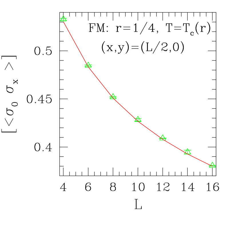
Figure 1: Triangles: averaged correlation functions for FM model at criticality (see Eqs. (7)and (8) ). Error bars are twice the standard deviation among three independent runs. Continuous line connects pure-system results for infinite strips, i.e. calculated with $\tilde{\psi}$, $\psi$ of Eq. (6) as the dominant left and right eigenvectors of the TM.

IV Numerical results for $\pm J$ Ising spin glass on strips

We now return to spin glasses. We first note that the pairing of successive odd and even moments predicted in Eq. (3) implies that

$$\left[C_{ij}^{\,(2\ell+1)}\right]-\left[C_{ij}^{\,(2\ell+2)}\right]=\hskip 128.0374pt$$

$$=\int_{-1}^{1}C_{ij}^{\,(2\ell+1)}\,(1-C_{ij})\,P(C_{ij})\ dC_{ij}\equiv 0\ .$$ (9)

Since this holds for any $\ell$, $P^{\prime}(C_{xy})\equiv(1-C_{xy})\,P(C_{xy})$ must be an even function of $C_{xy}$, everywhere on the NL. For the time being, we shall only consider $y=0$. Fig. 2, where results at the CNP for $L=4$, $8$, and $12$, $(x,y)=(L/2,0)$ are displayed, illustrates that such parity property is present, apart from small fluctuations caused by finite-sample and binning effects. The quantity $\Delta=\Delta(C)\equiv P^{\prime}(C_{xy})-P^{\prime}(-C_{xy})$ provides a quantitative measure of these deviations. With ${\overline{\Delta^{k}}}\equiv[\,(N_{\rm bin}/2)^{-1}\,\sum_{C=0}^{1}[\Delta(C)]^{k}\,]^{1/k}$, we find that: (i) for $N=2\times 10^{6}$, $|{\overline{\Delta^{1}}}|\leq 10^{-6}$ and ${\overline{\Delta^{2}}}\simeq 2\times 10^{-5}$, constant against $L$; and (ii) for fixed $L=4$ (where lattice structure has more pronounced effects, see Fig. 2, thus one would expect the most unfavorable environment for measuring such small fluctuations) and $10^{4}\leq N\leq 10^{7}$, ${\overline{\Delta^{2}}}$ varies roughly as $N^{-1/2}$. The latter is to be expected if deviations from parity arise from (randomly) incomplete sampling. Therefore, we can be confident that the property given in Eq. (3) is satisfied by our data, except for small random deviations whose origin is well understood. For $N=2\times 10^{6}$ samples and $4\leq L\leq 12$ the quantitative effect of such deviations on the moments of the distribution is that, for $0\leq\ell\leq 3$, Eq. (3) is satisfied to within one part in $10^{4}$. This holds not only for the $y=0$ data shown above, but for all relative positions $(x,y)$ investigated here (to be discussed below).

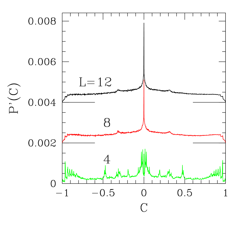
Figure 2: Data taken at the CNP. $P^{\prime}(C)\equiv(1-C)\,P(C)$, where $P(C)$ is the normalized histogram of occurrence of correlation function $C$. Strip widths $L=4$, $8$ and $12$ (the latter two vertically shifted respectively by 0.002 and 0.004, to avoid superposition); spin-spin relative positions ($x=L/2,y=0$). $N=2\times 10^{6}$ non-overlapping samples, for all cases.

As regards conformal invariance, we first recall that, for pure Ising systems on a strip of width $L$ with periodic boundary conditions across, the following result holds at criticality cardy :

$$C_{xy}^{\rm pure}\sim\left[\frac{\pi/L}{\left(\sinh^{2}(\pi x/L)+\sin^{2}(\pi y/L)\right)^{1/2}}\right]^{\eta}\ \ ,\ \ \eta=1/4,$$ (10)

where the proportionality factor can be obtained from the exact square–lattice ($L,R\to\infty,\ R\ll L$) result wu76 , $C_{R}=0.703\,38/R^{1/4}$. Though strictly speaking Eq. (10) is an asymptotic form, we have checked that discrepancies are already very small at short distances: for an $L=20$ strip, the largest deviation to be found between that and numerically-calculated values is $1.3\%$ for $(x,y)=(1,1)$, while it remains below $0.5\%$ for all other cases, approaching zero very fast: for $(x,y)=(3,3)$ it is $0.2\%$. The picture is the same already for smaller strip widths, e.g. $L=10$.

Figure 3: Differences ${\cal D}_{i}$ between symmetrized distribution functions $P^{\prime}(C_{xy})-P^{\prime}(C_{x^{\prime}y^{\prime}})$ ( $P^{\prime}(C)\equiv(1-C)\,P(C)$, where $P(C)$ is the normalized histogram of occurrence of correlation function $C$). ${\cal D}_{1}=P^{\prime}(C_{15})-P^{\prime}(C_{23})$, ${\cal D}_{2}=P^{\prime}(C_{15})-P^{\prime}(C_{51})$; insert(same scale as main plot): ${\cal D}_{3}=P^{\prime}(C_{23})-P^{\prime}(C_{32})$. Data taken at the CNP for strip width $L=10$, $N=2\times 10^{6}$ non-overlapping samples in all cases. Dashed horizontal lines at $\pm{\overline{\Delta^{2}}}$ (rms deviation of $P^{\prime}(C)$ from parity for $N$ as given above, see text).

Turning to disordered systems, a version of Eq. (10) was used at the NP in the strip calculations of Ref. picco, . Moments of order $i=1,2,\cdots 8$ of the correlation function distribution, for $y=0$ and varying $x\leq L$, were numerically calculated and fitted to the form Eq. (10), with the corresponding $\eta_{i}$ to be extracted from the fitting procedure. For $i=1$ their result is $\eta_{1}=0.1854$ (error bar estimated as $\simeq 1\%$ picco ), which agrees with, and is more accurate than, that obtained from the asymptotic decay of correlations, namely 0.182(5) sbl3 .

Here we shall try to capture variations in the correlation function distribution and its moments, against variations in the argument of Eq. (10), $z\equiv(\sinh^{2}(\pi x/L)+\sin^{2}(\pi y/L))^{1/2}$. As (i) the coordinates $(x,y)$ only take discrete values, and (ii) we have no guide as to the specific functional dependence of $P(C_{xy})$ on $z$, we shall at first compare distributions corresponding to points for which the argument is nearly equal, in contrast to those corresponding e.g. to the same distance, but with significantly different arguments. We take $L=10$ and the points $(x,y)=(1,5)$, $(2,3)$, $(3,2)$ and $(5,1)$, for which one has $z_{23}/z_{15}=1.001$; $z_{51}/z_{15}=2.1922$; $z_{32}/z_{23}=1.1773$.

In Fig. 3 we show the differences between pairs of symmetrized distributions $P^{\prime}(C_{xy})$: ${\cal D}_{1}=P^{\prime}(C_{15})-P^{\prime}(C_{23})$, ${\cal D}_{2}=P^{\prime}(C_{15})-P^{\prime}(C_{51})$, ${\cal D}_{3}=P^{\prime}(C_{23})-P^{\prime}(C_{32})$. Indeed, the differences between distributions behave qualitatively as one would expect, should the dependence on $x$ and $y$ be only through $z$. The horizontal lines at $\pm{\overline{\Delta^{2}}}$ (rms deviation of $P^{\prime}(C)$ from parity for $N=2\times 10^{6}$ as is the case here) show that, for ${\cal D}_{1}$ the $0.1\%$ difference in the respective arguments of $z$ gives rises to effects of the same order of magnitude as those arising from each individual distribution’s deviations from parity.

A more quantitative perspective can be obtained by analysing the dependence of assorted moments $m_{i}$ of the distribution against $z$. In Fig. 4 we show odd moments of the correlation function distribution at the CNP, for $L=10$ and $1\leq x\leq 3$, $0\leq y\leq 5$. These correspond to a region where the argument $z$ is strongly influenced by $y$, thus it is especially convenient for the discussion of the angular dependence implied in Eq. (10).

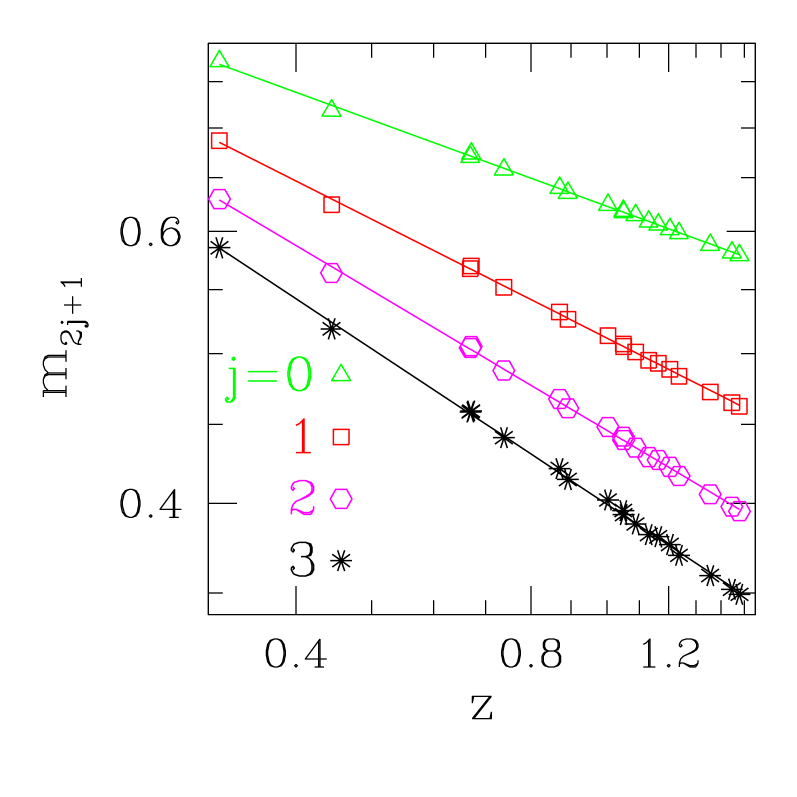
Figure 4: Double-logarithmic plot of odd moments of the correlation-function distribution $P(C_{xy})$ against $z\equiv(\sinh^{2}(\pi x/L)+\sin^{2}(\pi y/L))^{1/2}$; $1\leq x\leq 3$, $0\leq y\leq 5$. Straight lines are unweighted least-squares fits to data. Data taken at the CNP for strip width $L=10$, $N=3\times 10^{6}$ non-overlapping samples in all cases.

From the data displayed above, the overall conclusion is that conformal invariance holds at the NP, in the strict angle-dependent form corresponding to Eq. (10). Note that the point $(x,y)=(1,1)$, $z=1.0943$, for which the discrepancy between numerically-calculated value and asymptotic expression of correlation function is the largest for pure systems, also corresponds to the largest deviation from least-squares fitting lines in the disordered case.

We now turn to the question of whether the location of the NP, as conjectured in Refs. nn02, ; mnn03, , may be exact. We investigate the numerical values of the exponents $\eta_{\,2j+1}$, as obtained from the moments of the correlation-function distribution. We have performed least-squares fits of data for fixed $L=10$ with the grid of $z-$values shown in Fig. 4 (henceforth called $z-$fits), to the form suggested by Eq. (10) for this case, namely $m_{2j+1}\sim z^{-\eta_{\,2j+1}}$. We have scanned the NL in the immediate neighborhood of the CNP, $0.8886\leq p\leq 0.8914$, so as to include the uncertainty ranges of some recent estimates for the location of the NP picco ; mc02a ; ozeki . We found that the quality of fits, as given by the corresponding chi-square, does not change noticeably along that interval. Our estimates are displayed in Fig. 5, where the pairs of dashed lines in the central region of the Figure show ranges of exponent estimates given in Ref. picco, , namely $\eta_{\,2j+1}=0.1854$, $0.2561$, $0.3015$, $0.3354$ for $j=0$, $1$, $2$, $3$ (error bars assumed to be $1\%$ picco ). One sees that the results of $z-$fits are closest to those of Ref. picco, at the CNP, not at the location of the NP predicted in that reference.

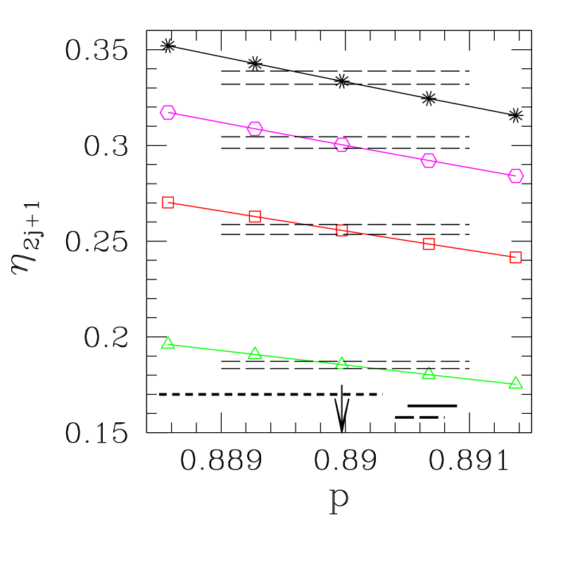
Figure 5: Results of least-squares fits of odd moments of the correlation-function distribution $P(C_{xy})$ to the form Eq. (10), with the $\eta_{i}$ as parameters; $L=10$, $1\leq x\leq 3$, $0\leq y\leq 5$, $N=3\times 10^{6}$ non-overlapping samples in all cases. Data taken along the NL, parametrized by ferromagnetic bond concentration $p$. Key to symbols is the same as in Fig. 4 (bottom to top: $j=0$, $1$, $2$, $3$). Error bars are of same order as symbol sizes. Vertical arrow: location of CNP. Heavy horizontal lines close to bottom show ranges of some recent estimates for location of NP. Long dashes: Ref. picco, ; full line: Ref. mc02a, ; short dashes: Ref. ozeki, . Pairs of dashed lines show ranges of exponent estimates given in Ref. picco, .

Table 1: Estimates of exponents $\eta_{\,2j+1}$, from least-squares fits of averaged odd moments of correlation-function distributions; $z-$fit: data for $L=10$ and $1\leq x\leq 3$, $0\leq y\leq 5$, assuming $m_{2j+1}\sim z^{-\eta_{\,2j+1}}$; $L=4-12$: data for $x=L/2$, $y=0$, assuming $m_{\,2j+1}\sim L^{-\eta_{\,2j+1}}$. First and second columns: data taken at the CNP. Third and fourth columns: pure system at criticality. Uncertainties in last quoted digits are shown in parentheses.

CNP

Pure

$j$	$z-$fit	$L=4-12$	$z-$fit	exact
0	0.1854(17)	0.1851(20)	0.2497(24)	1/4
1	0.2556(20)	0.2573(32)	0.7528(79)	3/4
2	0.300(2)	0.298(4)	1.265(15)	5/4
3	0.334(3)	0.325(5)	1.792(27)	7/4

In order to infer how much systematic error is implicit in the $z-$fitting procedure, we (i) performed least-squares fits of data taken at the CNP for $4\leq L\leq 12$, $x=L/2$, $y=0$ against the form suggested by Eq. (10) for that case, i.e. $m_{2j+1}\sim L^{-\eta_{\,2j+1}}$; and (ii) took pure-system data at criticality, from the same grid of $z-$ values used at the NP, and extracted the corresponding estimates of $\eta_{\,2j+1}$ from $z-$ fits. The results of (i) and (ii) are shown respectively in the second and third columns of Table 1.

From the analysis of pure-system data in Table 1 we conclude that, at least for $j=0$ and $1$, the intrinsic inaccuracy of $z-$fits does not significantly compromise our final results. For these same values of $j$, we also find greater internal consistency between $z-$ fit and $L=4-12$ estimates at the CNP. This signals that finite-width effects are essentially subsumed in the explicit $L-$ dependence given in Eq (10), i.e. higher-order finite-size corrections presumably do not play a significant role. Of course, a decisive test of the latter statement would involve e.g. doing $z-$fits on significantly wider strips.

For the moment, the data at hand allow us only to conclude that the conjectured exact location of the NP, as given in Refs. nn02, ; mnn03, , cannot be definitely ruled out. On the contrary, if we assume that the numerical values of the $\eta_{i}$ given in Ref. picco, are the most reliable ones at present, then our results are in fact consistent with the conjecture.

V Approximate scaling

In order to further understand the properties (so far, numerically found) of correlation function distributions, in this section we introduce an approximate scaling transformation which incorporates the gauge symmetries underlying the NL .

We recall, from real-space renormalization ideas, the concept of decimation sw76 ; ys76 ; rbs83 : considering e.g. a square lattice, summing upon the degrees of freedom of spins on a given sublattice will produce a new square lattice with half as many sites as the original one, and a lattice parameter enlarged by a factor of $\sqrt{2}$. In this context, the appropriate variable is the bond transmissivity $t\equiv\tanh(J/T)$, which represents the spin-spin correlation function in a restricted (single-bond) ensemble. For a point on the NL, the constraint given in Eq. (2) means that, with $t_{0}\equiv\tanh(J_{0}/T)$, the probability distribution of $t$ is

$${\cal P}(t)=\frac{1}{2}(1+t_{0})\,\delta(t-t_{0})+\frac{1}{2}(1-t_{0})\,\delta(t+t_{0})\ .$$ (11)

Denoting by $t_{i},\ i=1,2,3,4$ the transmissivities of bonds around a plaquette, the scaled transmissivity of the diagonal (effective) bond after decimation is ys76 ; rbs83

$$t^{\prime}=\frac{t_{1}t_{2}+t_{3}t_{4}}{1+t_{1}t_{2}t_{3}t_{4}}\ .$$ (12)

We investigate how the distribution function of scaled transmissivities, ${\cal P}(t^{\prime})$, evolves under successive rescalings via Eq. (12), given that the original distribution obeys Eq. (11).

We first prove that the distributions generated by iteration of Eq. (12) obey the NL symmetry given in Eq. (3), i.e. the NL is an invariant subspace of the transformation Eq. (12). The proof is by induction, as follows.

(i) Direct examination of Eq. (11) shows that the moments $m^{(0)}_{j}$ of the original, i.e. zero-th order distribution, obey

$$m^{(0)}_{2\ell+1}\equiv\left[t^{2\ell+1}\right]^{(0)}=m^{(0)}_{2\ell+2}\equiv\left[t^{2\ell+2}\right]^{(0)}\ ,$$ (13)

where the upper index $(0)$ attached to square brackets denotes average over the distribution Eq. (11).

(ii) Assuming that $m^{(n)}_{2\ell+1}=m^{(n)}_{2\ell+2}$, whence $\left[t^{2\ell+1}\,(1-t)\right]^{(n)}=0$, where the upper index $(n)$ denotes averages over the $n$–th order iterated distribution, one can show that

$$\left[t^{2\ell+1}\,(1-t)\right]^{(n+1)}=\hskip 136.5733pt$$

$$=\left[\left(\frac{t_{1}t_{2}+t_{3}t_{4}}{1+t_{1}t_{2}t_{3}t_{4}}\right)^{2\ell+1}\left(1-\frac{t_{1}t_{2}+t_{3}t_{4}}{1+t_{1}t_{2}t_{3}t_{4}}\right)\right]^{(n)}\equiv 0\quad$$ (14)

by expanding the RHS and invoking the statistical independence of the variables $t_{i}$.

In fact, the invariance property just proved is guaranteed by Eq. (12), because the decimated spins are connected to an even number of bonds. Indeed, the gauge transformation originally introduced for the $\pm 1/2$ Ising spins, in the derivation of the NL nish81 ; nish02 , could equally well have been applied to the transmissivities of the current approach, with the same final result.

Analytical examination of the evolution of ${\cal P}(t)$ under iteration of Eq. (12) shows the following relevant features:

(1) Assuming that the distribution has a non-negligible weight near $t=0$ and making a self-consistent ansatz, in which ${\cal P}^{(n)}(t)\sim t^{\alpha^{(n)}}$, one obtains the fixed-point value $\alpha^{\ast}=-1$, i.e. ${\cal P}(t)\sim|t|^{-1}$, $t\to 0$.

(2) Assuming now that the distribution has a non-negligible weight near $t=1$, and making an ansatz in which, with $\delta\equiv 1-t$, ${\cal Q}^{(n)}(\delta)={\cal P}^{(n)}(1-t)\sim\delta^{\beta^{(n)}}$, one obtains the fixed-point value $\beta^{\ast}=-1$, i.e. ${\cal P}(t)\sim(1-t)^{-1}$, $t\to 1$.

The analytic predictions for the exponent values $\alpha^{\ast}$, $\beta^{\ast}$ were determined by the limiting forms of Eq. (12) for small $t_{i}$ or small $1-t_{i}$ respectively. Of these, the first is the less reliable, since the simple transformation Eq. (12) captures less well the key subtle effects needed there, of removal of order by frustration, than the simpler characteristics of the ferromagnetic state involved at small $1-t_{i}$. So we expect (and find, see below) that the predicted $\alpha^{\ast}$ is much less reliable than the predicted $\beta^{\ast}$.

In order to test the above predictions, one might work out the iterated distributions directly from Eq. (12). This, however, is feasible only for the first four iterations, since the number of distinct outcomes grows very rapidly from 2 of Eq. (11) at order zero, respectively to 3, 5, 25, 702 at subsequent orders (the latter figure, for the fourth-order distribution, reflects the binning of $25^{4}=390,625$ results onto $10^{3}$ bins of width $2\times 10^{-3}$, while no binning was used for the preceding iterations). The next step would involve considering of order $2\times 10^{11}$ operations, which might be reduced by perhaps one order of magnitude by considering symmetries. The alternative of considering a coarser binning structure (to be kept fixed for iterations of order $\geq 4$) was seen to introduce gross distortions of the symmetry reflected in Eq. (3), thus the presumptive advantages of exact recursion relations over the purely numerical techniques of section IV would be lost.

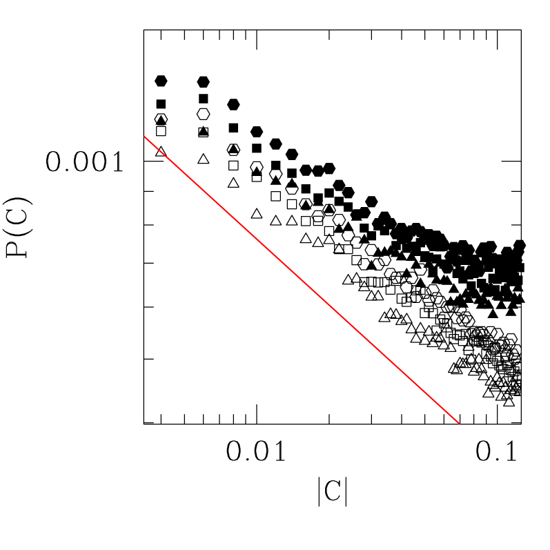
Figure 6: Double-logarithmic plot of $P(C)$ close to $C=0$. Full symbols: $C>0$; empty symbols: $C<0$ (divided by $1.10$, to reduce superposition). Strip widths $L=8$ (triangles)), $10$ (squares), and $12$ (hexagons). For all cases, $x=L/2$, $y=0$. Straight line corresponds to $P(C)\sim|C|^{-1/3}$. Data taken at the CNP.

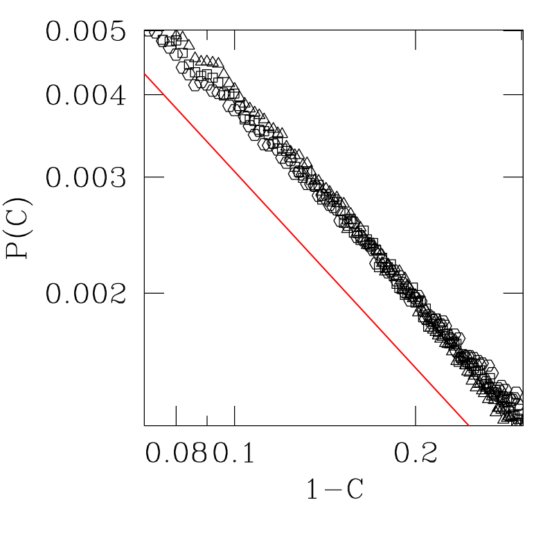
Figure 7: Double-logarithmic plot of $P(C)$ close to $C=1$. Strip widths $L=8$ (triangles)), $10$ (squares), and $12$ (hexagons). For all cases, $x=L/2$, $y=0$. Straight line corresponds to $P(C)\sim(1-C)^{-1}$. Data taken at the CNP.

Before setting out to compare predictions (1) and (2) to numerically-collected data on strips, we mention that the soundness of the rescaling scheme can be roughly tested as follows. Following the usual renormalization-group ideas, one would expect the NP to be characterized by a scaling-invariant ${\cal P}^{\ast}(t)$ rbs83 . In practice, one searches for equality between the $j$–th moments of the $m$–th and $n$–th order iterated distributions, expecting that the results (i) do not depend strongly on the choice of $j$, and (ii) should improve as $m$ and/or $n$ grows. Considering $m=0$, one can parametrize the search for a fixed point distribution through the value $t_{0}$ in Eq. (11): for $t_{0}=t_{0}^{\ast}$, $m^{(0)}_{j}=m^{(n)}_{j}$. In this context, recalling the invariance of the NL under Eq. (12) and taking $j=1$, we have $p^{\ast}=p(t_{0}^{\ast})=0.9395$ and $0.9417$, respectively for $n=3$ and $4$. An ad hoc two-point extrapolation against $1/n$ gives a non-trivial limiting value, $\lim_{\ n\to\infty}p^{\ast}=0.959$. This is to be compared with the presumed exact $p=0.889972\cdots$ nn02 ; mnn03 . We conclude that the rescaling scheme is qualitatively correct, though its quantitative predictions must be carefully scrutinized.

We have tested prediction (1) above against numerical data from strips. The results are displayed in Fig. 6. One can see that, although there are clear signs of a power-law divergence both below and above $C=0$, the corresponding exponent is certainly not above $1/3$. The slight asymmetry between data for $C>0$ and $C<0$ is entirely consistent with the general property that the symmetrized distribution $P^{\prime}(C)$ is an even function. Indeed, by plotting $P^{\prime}(C)$ we get two essentially identical branches. Turning now to prediction (2), the corresponding results are displayed in Fig. 7. Now one can see that the form $P(C)\sim(1-C)^{-1}$ indeed captures the essential features of behavior.

VI Conclusions

Our investigation has probed behavior at the Nishimori point (NP), where the infinite two-dimensional system is both critical and subject to the Nishimori gauge symmetry. Mounting, but incomplete, evidence has suggested that random critical two-dimensional systems share, in a statistical sense, the conformal invariance of their pure counterparts. So it was expected that at the NP, the correlation function distributions $P(C)$ on strips would be the same at all (lattice) points $(x,y)$ on any curve of constant $|\,\sinh(\pi(x+iy)/L)\,|$ (see Eq. (10)). Evidence has been presented in section IV that this strict form of statistical conformal invariance indeed applies. This is especially important here, since all numerical evidence available so far, regarding conformal-invariance properties at the NP, points to values of e.g. the exponents $\eta_{i}$ and the central charge which are not obviously associated to any previously known universality class sbl3 ; picco ; mc02a . Our data do not rule out the possibility that the recently-conjectured location of the NP, at the intersection of Eqs. (2) and (4), is indeed exact.

Among other results are the power-law divergencies of distributions $P(C)$ near $C=1$ and $C=0$, which were first identified in the invariant distributions of the simple scaling theory (section V) and then confirmed by the strip scaling analysis (section V). Of the respective power laws ($-1$, $-1/3$) only the first was correctly predicted because of the crudeness of the scaling transformation, Eq. (12) (which nevertheless maintains the gauge symmetry).

- (1) H. Nishimori, Prog. Theor. Phys. 66 1169 (1981).
- (2) H. Nishimori, Statistical Physics of Spin Glasses and Information Processing: An Introduction (Oxford University Press, Oxford, 2001).
- (3) H. Nishimori and K. Nemoto, J. Phys. Soc. Jpn. 71, 1198 (2002).
- (4) J.-M. Maillard, K. Nemoto, and H. Nishimori, cond-mat/0306154 (2003).
- (5) H. Nishimori, J. Phys. Soc. Jpn. 55, 5305 (1986).
- (6) H. Nishimori, J. Phys. A 35, 9541 (2002).
- (7) P. Le Doussal and A. B. Harris, Phys. Rev. Lett. 61, 625 (1988).
- (8) R. R. P. Singh and J. Adler, Phys. Rev. B54, 364 (1996)
- (9) N. Kawashima and H. Rieger, Europhys. Lett. 39, 85 (1997).
- (10) J. A. Blackman, J. R. Gonçalves, and J. Poulter, Phys. Rev. E58 1502 (1998).
- (11) F. D. A. Aarão Reis, S. L. A. de Queiroz, and R. R. dos Santos, Phys. Rev. B60, 6740 (1999).
- (12) A. Honecker, M. Picco, and P. Pujol, Phys. Rev. Lett. 87, 047201 (2001).
- (13) F. Merz and J. T. Chalker, Phys. Rev. B65, 054425 (2002).
- (14) N. Ito and Y. Ozeki, Physica A 321, 262 (2003).
- (15) E. Domany, J. Phys. C 12, L119 (1979).
- (16) J. L. Cardy, in Phase Transitions and Critical Phenomena, edited by C. Domb and J. L. Lebowitz (Academic, New York, 1987), Vol. 11.
- (17) S. L. A. de Queiroz, Phys. Rev. E51, 1030 (1995).
- (18) S. L. A. de Queiroz and R. B. Stinchcombe, Phys. Rev. E54, 190 (1996).
- (19) S. L. A. de Queiroz, J. Phys. A 30, L447 (1997).
- (20) For a recent review, see B. Berche and C. Chatelain, cond-mat/0207421 (lectures given at ICMP, Lviv, Ukraine).
- (21) F. Iglói and H. Rieger, Phys. Rev. Lett. 78, 2473 (1997).
- (22) J. L. Cardy, J. Phys. A 17, L385 (1984).
- (23) M. P. Nightingale, in Finite Size Scaling and Numerical Simulations of Statistical Systems, edited by V. Privman (World Scientific, Singapore, 1990).
- (24) R. Fisch, J. Stat. Phys. 18, 111 (1978).
- (25) W. Kinzel and E. Domany, Phys. Rev. B23, 3421 (1981).
- (26) A. L. Talapov and L. N. Shchur, Europhys. Lett. 27, 193 (1994).
- (27) T. T. Wu, B. M. McCoy, C. A. Tracy, and E. Barouch, Phys. Rev. B13, 316 (1976).
- (28) R. B. Stinchcombe and B. P. Watson, J. Phys. C 9, 3221 (1976).
- (29) A. P. Young and R. B. Stinchcombe, J. Phys. C 9, 4419 (1976).
- (30) R. B. Stinchcombe, in Phase Transitions and Critical Phenomena, edited by C. Domb and J. L. Lebowitz (Academic, New York, 1983), Vol. 7.