Diffuse waves in nonlinear disordered media⁰

I Introduction

The field of multiple scattering of classical waves (electromagnetic, acoustic and elastic waves, etc.) in disordered media has revived in the eighties albada85 –sheng90 , when the far-reaching analogies between the diffuse transport of waves and electrons in mesoscopic systems have been realized (see Ref. tiggelen94 for a comprehensive review of the latter issue). Using classical waves to study such phenomena as weak and strong localization, mesoscopic correlations and universal conductance fluctuations (see Refs. berk94 –sebbah01 for reviews) appears to be advantageous in many aspects: no need for low temperatures and small samples, better control of the experimental apparatus, possibility of more sensitive measurements, etc. In addition, experiments with classical waves can be readily performed in the linear regime, excluding interaction between scattered waves and hence simplifying the interpretation of experimental data, whereas the electron-electron interaction is always present in the realm of mesoscopic electronics and cannot simply be ‘turned off’, introducing significant difficulties in the theoretical model alt91 .

The ‘interaction’ of classical waves, analogous in some sense to the electron-electron interaction, can come about if the waves propagate in a nonlinear medium. Such an interaction is a matter of scientific enquiry in the fields of nonlinear optics boyd02 , nonlinear acoustics hamilton78 , etc. Nowadays, the latter are rapidly developing scientific disciplines on their own right, having considerable fundamental importance and numerous practical applications. Various nonlinear phenomena (self-action: self-phase modulation and self-focusing of pulses and beams, harmonic generation, shock wave formation, etc.) occur in homogeneous nonlinear media depending on the type and strength of the nonlinearity. The effect of weak disorder on the propagation of nonlinear waves has also been studied both theoretically (treating it as a weak perturbation) and experimentally (e.g., for laser beam propagation through atmospheric turbulence) kandidov96 . Unfortunately, only few experiments boer93 have been performed up to now on multiple, diffuse scattering of classical waves in nonlinear media. Theoretical analysis of the problem is more advanced (see the bibliography of Ref. skip00 ), but is still insufficient to stimulate further experimental effort. Meanwhile, diffuse waves seem to be a good candidate for a detailed study of the combined effect of disorder and nonlinearity (or interaction) on wave (or quantum particle) propagation, as compared to interacting electrons in disordered mesoscopic samples: the strength and the type of nonlinear wave ‘interaction’ can be readily controlled and the nonlinear term in the wave equation is often of simple algebraic form. Despite these important simplifications, diffusion of classical waves in nonlinear media remains an involved problem and is far from being solved. The purpose of the present paper is to review our recent theoretical results skip00 –skip02b which are particularly susceptible to stimulate the reader’s interest, further theoretical analysis, and, hopefully, new experiments.

For the sake of concreteness, we restrict our consideration to the problem of self-action of a scalar monochromatic wave (frequency $\omega$) in a nonlinear disordered medium. This is described by the following wave equation:

$$\left\{\nabla^{2}-\frac{1}{c^{2}}\frac{\partial^{2}}{\partial t^{2}}\left[1+\delta\varepsilon({\mathbf{r}})+\Delta\varepsilon_{\mathrm{NL}}({\mathbf{r}},t)\right]\right\}E({\mathbf{r}},t)$$

$$\hskip 56.9055pt=J({\mathbf{r}},t),$$ (1)

where $E({\mathbf{r}},t)$ is the wave amplitude, $c$ is the speed of the wave in the average medium, $J({\mathbf{r}},t)=J_{0}({\mathbf{r}})$ $\exp(-i\omega t)$ is a monochromatic source term, $\delta\varepsilon({\mathbf{r}})$ is the fractional fluctuation of the linear dielectric constant, and the nonlinear part of the dielectric constant $\Delta\varepsilon_{\mathrm{NL}}({\mathbf{r}},t)$ depends on the intensity $I({\mathbf{r}},t)=\left|E({\mathbf{r}},t)\right|^{2}$ of the wave. Eq. (1) describes, e.g., propagation of light in a medium with intensity-dependent refractive index and (as the reader might already have noted) we adopt the ‘optical’ terminology from here on. Furthermore, we consider $E$ in Eq. (1) to be a complex quantity, thus neglecting the (possible) generation of the third harmonics, and restrict ourselves to a weak nonlinearity (see below for the definition of ‘weakness’).

There are two fundamental questions to consider concerning the propagation of waves in a disordered medium with a weak nonlinearity. First, one can ask about the effect of nonlinearity on the phenomena known for waves in linear disordered media. We partially answer this question in Sec. IV, where we summarize the results of calculation of the angular correlation functions of scattered waves and the analysis of the coherent backscattering cone in a nonlinear disordered medium. The second question is more challenging: can the weak nonlinearity give rise to new physical phenomena which are not present in the linear medium? The answer to the latter question is ‘yes’ as we demonstrate in Sec. V where the instability of diffuse, multiple-scattered waves in a disordered medium with a weak nonlinearity is considered. In order to facilitate the presentation of our main results, we start by a very brief review of principal results known for waves in linear disordered (Sec. II) and homogeneous nonlinear (Sec. III) media.

II Waves in Linear Disordered Media

Waves propagating in a linear disordered medium are described by Eq. (1) with $\Delta\varepsilon_{\mathrm{NL}}({\mathbf{r}},t)=0$. Despite its linearity, this problem is a rather involved one and it attracts a lot of attention (see, e.g., the articles in the present book and Refs. rossum99 and sebbah01 ). In what follows, we are interested uniquely in the diffusion regime of wave propagation that is realized for $k_{0}\ell\gg 1$, where $k_{0}=\omega/c$ and $\ell$ is the mean free path due to disorder. To simplify still further the consideration, we assume that the correlation length of $\delta\varepsilon({\mathbf{r}})$ is much shorter than the wavelength $\lambda$ and adopt the model of the Gaussian white-noise disorder: $\left<\delta\varepsilon({\mathbf{r}})\delta\varepsilon({\mathbf{r}}_{1})\right>=4\pi/(k_{0}^{4}\ell)\delta({\mathbf{r}}-{\mathbf{r}}_{1})$, so that the scattering and the transport mean free paths coincide. Besides, we consider a disordered medium without absorption (i.e. both $\delta\varepsilon$ and $\Delta\varepsilon_{\mathrm{NL}}$ are real), except if the opposite is specified explicitly. In the regions of space located at distances greater than $\ell$ from the sources of waves and the boundaries of the sample, the average intensity $\left<I({\mathbf{r}})\right>$ then obeys a diffusion equation ishim78 :

$$\frac{\partial}{\partial t}\left<I({\mathbf{r}},t)\right>=D\nabla^{2}\left<I({\mathbf{r}},t)\right>+S({\mathbf{r}},t),$$ (2)

where $D=c\ell/3$ is the diffusion constant and $S({\mathbf{r}},t)$ is the source term. In the following, we assume a time-independent source term in Eq. (2): $S({\mathbf{r}},t)=S({\mathbf{r}})$, yielding $I({\mathbf{r}},t)=I({\mathbf{r}})$.

The average intensity $\left<I({\mathbf{r}})\right>$ given by Eq. (2) is not sufficient to describe the intensity $I({\mathbf{r}})$ of the wave, since the latter exhibits large fluctuations: $\delta I({\mathbf{r}})=I({\mathbf{r}})-\left<I({\mathbf{r}})\right>\sim\left<I({\mathbf{r}})\right>$ ishim78 ; shapiro86 . The spatial correlation function of $\delta I({\mathbf{r}},t)$ contains a short-range ($\Delta r<\ell$) but strong ($\sim 1$) contribution shapiro86 :

$$\left<\delta I({\mathbf{r}})\delta I({\mathbf{r}}_{1})\right> = \left<I({\mathbf{r}})\right>\left<I({\mathbf{r}}_{1})\right>\left[\frac{\sin(k_{0}\Delta r)}{k_{0}\Delta r}\right]^{2}$$ (3)

$$\times \exp\left(-\frac{\Delta r}{\ell}\right)$$

and a long-range ($\Delta r>\ell$) but weak [$\sim(k_{0}\ell)^{-2}\ll 1$] contribution stephen87 ; zyuzin87 :

$$\left<\delta I({\mathbf{r}})\delta I({\mathbf{r}}_{1})\right>\sim\frac{c}{k_{0}^{2}}I_{0}^{2}G({\mathbf{r}},{\mathbf{r}}_{1})\sim\frac{I_{0}^{2}}{k_{0}^{2}\ell\Delta r},$$ (4)

where $\Delta{\mathbf{r}}={\mathbf{r}}-{\mathbf{r}}_{1}$, $I_{0}$ is a typical value of $\left<I({\mathbf{r}})\right>$, $G({\mathbf{r}},{\mathbf{r}}_{1})$ is the Green’s function of Eq. (2) with $(\partial/\partial t)=0$, and the last expression in Eq. (4) is obtained assuming that $G({\mathbf{r}},{\mathbf{r}}_{1})$ is equal to its value in the infinite medium: $G({\mathbf{r}},{\mathbf{r}}_{1})=G_{0}({\mathbf{r}},{\mathbf{r}}_{1})=(4\pi D\Delta r)^{-1}$. The short-range contribution to the intensity correlation function (3) describes the speckle structure of the spatial intensity distribution in disordered media, while the long-range contribution (4) testifies that different speckle spots are correlated (weakly, since $k_{0}\ell\gg 1$). The correlation functions given by Eqs. (3) and (4) are commonly referred to as $C^{(1)}$ and $C^{(2)}$, respectively. Other contributions to the intensity correlation function can exist: $C^{(3)}$ is a factor $(k_{0}\ell)^{-2}\ll 1$ smaller than $C^{(2)}$ rossum99 and $C^{(0)}\sim(k_{0}\ell)^{-1}$ is non-vanishing only if the source of waves has the size smaller or of the order of the wavelength $\lambda$ shapiro99 . We do not consider the two latter contributions here.

Short- and long-range correlation functions of the field and intensity fluctuations can be also defined in the angular domain. For our purposes, it will be sufficient to consider only the short-range correlations $C^{(1)}$. If a plane wave is incident on a disordered slab of thickness $L\gg\ell$ (slab surfaces being perpendicular to the $z$-axis) with a wave vector ${\mathbf{k}}_{a}=\{{\mathbf{q}}_{a},k_{az}\}$, where ${\mathbf{q}}_{a}=\{k_{ax},k_{ay}\}$, the field (intensity) of the wave transmitted through the slab with a wave vector ${\mathbf{k}}_{b}$ is $E({\mathbf{k}}_{a},{\mathbf{k}}_{b})$ [$I({\mathbf{k}}_{a},{\mathbf{k}}_{b})=\left|E({\mathbf{k}}_{a},{\mathbf{k}}_{b})\right|^{2}$]. If the above experiment is repeated for different incoming and outgoing wave vectors ${\mathbf{k}}_{a}^{\prime}$ and ${\mathbf{k}}_{b}^{\prime}$, respectively, the normalized correlation function of scattered fields

$$C({\mathbf{k}}_{a},{\mathbf{k}}_{b};{\mathbf{k}}_{a}^{\prime},{\mathbf{k}}_{b}^{\prime}) \equiv C_{aba^{\prime}b^{\prime}}$$ (5)

$$= \frac{\left<E({\mathbf{k}}_{a},{\mathbf{k}}_{b})E^{*}({\mathbf{k}}_{a}^{\prime},{\mathbf{k}}_{b}^{\prime}\right>)}{\left<I({\mathbf{k}}_{a},{\mathbf{k}}_{b})\right>^{1/2}\left<I({\mathbf{k}}_{a}^{\prime},{\mathbf{k}}_{b}^{\prime})\right>^{1/2}}$$

appears to have a rather simple form berk94 :

$$C_{aba^{\prime}b^{\prime}}=\delta_{\Delta{\mathbf{q}}_{a},\Delta{\mathbf{q}}_{b}}F_{\mathrm{T}}(\Delta q_{a}L),$$ (6)

where $F_{\mathrm{T}}(x)=x/\sinh x$, $\Delta{\mathbf{q}}_{a}={\mathbf{q}}_{a}-{\mathbf{q}}_{a}^{\prime}$ (and similarly for $\Delta{\mathbf{q}}_{b}$), and $\Delta q_{a}\ell\ll 1$ is assumed.

The field correlation in reflection, when both incident and scattered waves are on the same side of the slab, is berk94 ; bressoux00

$$C_{aba^{\prime}b^{\prime}}\simeq\delta_{\Delta{\mathbf{q}}_{a},\Delta{\mathbf{q}}_{b}}\left[F_{\mathrm{R}}(\Delta{\mathbf{q}}_{a})+F_{\mathrm{R}}({\mathbf{q}}_{a}+{\mathbf{q}}_{b}+\Delta{\mathbf{q}}_{a})\right],$$ (7)

where

$$F_{\mathrm{R}}({\mathbf{q}})\simeq(1+2\zeta)-2(1+\zeta)^{3}q\ell+\ldots,$$ (8)

$\zeta\sim 1$ is the extrapolation factor ($\zeta=2/3$ in the diffusion approximation), $q\ell\ll 1$, and the semi-infinite disordered medium is considered. The short-range correlation function of intensity fluctuations, $C^{(1)}$, in transmission (reflection) geometry is obtained by taking the square of the absolute value of Eq. (6) [Eq. (7)].

Finally, a well-studied phenomenon in the linear disordered medium is the coherent backscattering albada85 , consisting in a two-fold (with respect to the incoherent, diffuse background) enhancement of the average scattered intensity in the direction of exact backscattering (${\mathbf{k}}_{b}=-{\mathbf{k}}_{a}$). For normal incidence (${\mathbf{q}}_{a}=0$), the angular line shape of the coherent backscattering cone can be approximately expressed using the function $F_{\mathrm{R}}$ defined in Eq. (8):

$$\frac{\left<I({\mathbf{q}})\right>}{\left<I_{\mathrm{inc}}\right>}\simeq\frac{F_{\mathrm{R}}(1/L_{\mathrm{a}})+F_{\mathrm{R}}[(q^{2}+1/L_{\mathrm{a}}^{2})^{1/2}]}{F_{\mathrm{R}}(1/L_{\mathrm{a}})},$$ (9)

where ${\mathbf{q}}\equiv{\mathbf{q}}_{b}$ and we have taken into account the absorption of light in the medium by introducing the macroscopic absorption length $L_{\mathrm{a}}\gg\ell$.

III Waves in Homogeneous Nonlinear Media

If $\delta\varepsilon({\mathbf{r}},t)=0$, Eq. (1) describes the propagation of waves in a homogeneous nonlinear medium (no scattering) with an intensity-dependent dielectric constant boyd02 . Below we consider the case of Kerr nonlinearity. If the nonlinear response of the medium is instantaneous and local, the dependence of $\Delta\varepsilon_{\mathrm{NL}}({\mathbf{r}},t)$ on $I({\mathbf{r}},t)$ is rather simple: $\Delta\varepsilon_{\mathrm{NL}}({\mathbf{r}},t)=\varepsilon_{2}I({\mathbf{r}},t)$, where $\varepsilon_{2}$ is a nonlinear coefficient. In general, however, the nonlinear response is not instantaneous and can be modeled by a phenomenological equation of Debye type for $\Delta\varepsilon_{\mathrm{NL}}$:

$$\tau_{\mathrm{NL}}\frac{\partial}{\partial t}\Delta\varepsilon_{\mathrm{NL}}({\mathbf{r}},t)=-\Delta\varepsilon_{\mathrm{NL}}({\mathbf{r}},t)+\varepsilon_{2}I({\mathbf{r}},t),$$ (10)

where $\tau_{\mathrm{NL}}$ is the response time of the nonlinearity. Moreover, the non-locality of the nonlinear response of the medium can be taken into account by considering $\Delta\varepsilon_{\mathrm{NL}}({\mathbf{r}},t)$ obeying an equation of diffusion type:

$$\tau_{\mathrm{NL}}\frac{\partial}{\partial t}\Delta\varepsilon_{\mathrm{NL}}({\mathbf{r}},t) = (a_{\mathrm{NL}})^{2}\nabla^{2}\left[\Delta\varepsilon_{\mathrm{NL}}({\mathbf{r}},t)\right]$$ (11)

$$- \Delta\varepsilon_{\mathrm{NL}}({\mathbf{r}},t)+\varepsilon_{2}I({\mathbf{r}},t),$$

where $a_{\mathrm{NL}}$ is some characteristic length, describing the degree of non-locality of the nonlinear response.

The physics of nonlinear optical phenomena in Kerr media is rather rich boyd02 and it is not our purpose to review it here. In the framework of our study, we would like, however, to call the attention of the reader to the following two simple but illustrative examples. First, if a nonlinear Kerr medium, illuminated by a monochromatic plane wave of intensity $I_{0}$, is put in an optical resonator, the feedback provided by the resonator leads to the instability of the steady-state solution $E({\mathbf{r}},t)=E_{0}({\mathbf{r}})\exp(-i\omega t)$ and the intensity $I=\left|E\right|^{2}$ of the wave develops a time dependence ikeda80 . This phenomenon occurs only at $I_{0}$ exceeding some threshold and the dynamics of $I({\mathbf{r}},t)$ becomes progressively more complex as $I_{0}$ increases. The second example concerns two counter-propagating light waves in a Kerr medium. Again, the steady-state solution develops an instability for the intensities of the waves exceeding a threshold silber82 . The above simple examples suggest that the unstable regimes are fundamental in nonlinear optics and this appears to be indeed true: instabilities, self-oscillations, pattern formation, and spatio-temporal chaos are observable in many nonlinear optical systems (see, e.g., Refs. gibbs85 –voron99 for reviews). Even incoherent light beams have been recently shown to exhibit pattern formation and ‘optical turbulence’ due to the so-called modulation instability soljacic00 , indicating that unstable behavior does not require the perfect coherence of the underlying wave field.

IV Angular Correlations and Coherent Backscattering for Waves in Nonlinear Disordered Media

After having briefly reviewed the key features of wave propagation in linear disordered and homogeneous nonlinear media, we are now in a position to attack the central problem of the present paper: diffuse wave propagation in nonlinear disordered media. A particularly pictorial description of the latter can be developed if the nonlinearity is assumed to be weak enough to have no significant effect on the general diffuse character of wave propagation in the medium and the values of the diffusion constant $D$ and the mean free path $\ell$. This requires the ‘nonlinear scattering length’ $\ell_{\mathrm{NL}}$ due to the nonlinear term in Eq. (1) to be much larger than $\ell$. $\ell_{\mathrm{NL}}$ can be estimated by assuming the short-range intensity correlation function in a nonlinear disordered medium to be approximately the same is in the linear one [see Eq. (3)]. Calculating the total scattering crossection of statistically isotropic fluctuations of the nonlinear dielectric constant $\varepsilon_{2}\delta I({\mathbf{r}})$ in the Born approximation, we obtain

$$\ell_{\mathrm{NL}}^{-1}\propto k_{0}^{2}\int_{0}^{2k_{0}}\Phi(\kappa)\kappa d\kappa,$$ (12)

where

$$\Phi({\mathbf{K}})\propto\varepsilon_{2}^{2}\int\left<\delta I({\mathbf{r}})\delta I({\mathbf{r}}+\Delta{\mathbf{r}})\right>\exp(-i{\mathbf{K}}\Delta{\mathbf{r}})d^{3}\Delta{\mathbf{r}},$$ (13)

and hence $\ell_{\mathrm{NL}}\sim(\Delta n^{2}k_{0})^{-1}$, where $\Delta n=n_{2}I_{0}$ is the typical value of the nonlinear correction to the refractive index, $n_{2}=\varepsilon_{2}/2$, and $I_{0}$ is the typical value of $\left<I({\mathbf{r}},t)\right>$. The condition of weak nonlinearity, $\ell\ll\ell_{\mathrm{NL}}$, then becomes

$$\Delta n^{2}k_{0}\ell\ll 1,$$ (14)

where, we recall, $k_{0}\ell\gg 1$. We adopt this condition throughout the rest of the paper.

We start the analysis of the effect of nonlinearity on multiple scattering of waves in disordered media by considering the angular correlation of scattered wave fields, $C_{aba^{\prime}b^{\prime}}$, as defined in Eq. (5) (Sec. II), assuming the two incident waves to have different amplitudes ($A$ for the wave with the wave vector ${\mathbf{k}}_{a}$ and $A^{\prime}$ for the wave with the wave vector ${\mathbf{k}}_{a}^{\prime}$). Due to the nonlinearity of the medium, $C_{aba^{\prime}b^{\prime}}$ will now depend not only on ${\mathbf{k}}_{a}$, ${\mathbf{k}}_{a}^{\prime}$, ${\mathbf{k}}_{b}$, and ${\mathbf{k}}_{b}^{\prime}$, but also on $A$ and $A^{\prime}$. For simplicity, we put $A^{\prime}\rightarrow 0$ (so that the effect of the nonlinearity on the propagation of the second wave is negligible) and limit ourselves to the case of instantaneous ($\tau_{\mathrm{NL}}=0$) local ($a_{\mathrm{NL}}=0$) nonlinearity.

The physical origin of the nonlinearity-induced modification of $C_{aba^{\prime}b^{\prime}}$ can be easily understood in the framework of the path-integral picture of wave propagation. The wave of amplitude $A$, propagating along some wave path of length $s$ through a nonlinear disordered medium, acquires an additional, ‘nonlinear’ phase shift $\Delta\phi_{\mathrm{NL}}$ with respect to the wave of amplitude $A^{\prime}\rightarrow 0$, propagating in an essentially linear medium:

$$\Delta\phi_{\mathrm{NL}}=k_{0}n_{2}\int_{0}^{s}ds_{1}I({\mathbf{r}}_{1}),$$ (15)

the average value of the latter being

$$\left<\Delta\phi_{\mathrm{NL}}\right>\approx k_{0}n_{2}A^{2}s,$$ (16)

where we assume $\left<I({\mathbf{r}}_{1})\right>\approx A^{2}$. In a linear medium, a similar phase difference arises between two waves at different frequencies $\omega\neq\omega^{\prime}$:

$$\Delta\phi_{\Delta\omega}=(\Delta\omega/c)s,$$ (17)

where $\Delta\omega=\omega-\omega^{\prime}\ll\omega$. It is well-known that the latter dephasing modifies the angular correlation function of scattered fields, which becomes (in transmission) berk94

$$C_{aba^{\prime}b^{\prime}}=\delta_{\Delta{\mathbf{q}}_{a},\Delta{\mathbf{q}}_{b}}F_{\mathrm{T}}\left[(\Delta q_{a}^{2}-2i\gamma^{2})^{1/2}L\right],$$ (18)

where $\gamma^{2}=3\Delta\omega/(2\ell c)$.

(a)

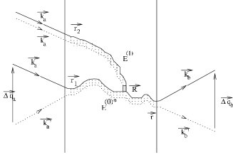
(b)

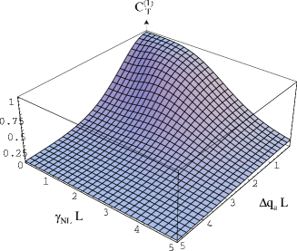
Figure 1: (a) The diagram contributing to the angular correlation function of scattered wave fields in a nonlinear disordered medium. (b) Short-range intensity correlation function for a diffuse wave transmitted through a slab. The figures are from Ref. [17].

The formal analogy between Eqs. (16) and (17) suggests that as long as the nonlinearity affects only the phase of the wave and not its amplitude (i.e. for a weak nonlinearity), the correlation function $C_{aba^{\prime}b^{\prime}}$ in a nonlinear disordered medium should be approximately given by Eq. (18), where $\Delta\omega$ is replaced by $\omega n_{2}A^{2}$. This is indeed confirmed by a perturbative diagrammatic calculation bressoux00 [see the diagram of Fig. 1(a)], that allows one to obtain the lowest term in the series expansion of $C_{aba^{\prime}b^{\prime}}$ in $n_{2}A^{2}\ll 1$. Applying then a ‘natural’ ansatz $f(x)-[i\epsilon^{2}/(2x)]f^{\prime}(x)\simeq f[(x^{2}-i\epsilon^{2})^{1/2}]$ yields bressoux00 :

$$C_{aba^{\prime}b^{\prime}}=\delta_{\Delta{\mathbf{q}}_{a},\Delta{\mathbf{q}}_{b}}F_{\mathrm{T}}\left\{\left[\Delta q_{a}^{2}L^{2}-2i(L/\xi)^{2}\right]^{1/2}\right\},$$ (19)

where $\xi$ is a new characteristic length, characterizing the damping of correlation due to the nonlinear effects:

$$\xi\approx\sqrt{\frac{\ell}{k_{0}\Delta n}}.$$ (20)

Here $\Delta n\approx n_{2}A^{2}$ is the typical value of the nonlinear part of the refractive index. The physical meaning of $\xi$ is clear: it is the characteristic length for the loss of phase coherence between two waves following the same diffusion path, one with a vanishing amplitude $A^{\prime}\rightarrow 0$ and the other one with a finite amplitude $A$. By analogy with the case of frequency correlation [Eq. (18)], $\gamma_{\mathrm{NL}}$ can be defined as $\gamma_{\mathrm{NL}}=1/\xi$. The short-range correlation function of intensity fluctuations, $C_{\mathrm{T}}^{(1)}$, can be obtained by taking a square of the absolute value of Eq. (19). We show this correlation function in Fig. 1(b).

Similarly to the case of transmission geometry, correlation between diffusely reflected waves can also be calculated taking into account the additional dephasing due to the nonlinearity of the medium. Again, assuming that the two incident waves have different amplitudes $A$ and $A^{\prime}\rightarrow 0$, one finds for a semi-infinite disordered medium bressoux00

$$C_{aba^{\prime}b^{\prime}}\simeq\delta_{\Delta{\mathbf{q}}_{a},\Delta{\mathbf{q}}_{b}}\left\{F_{\mathrm{R}}\left[\left(\Delta{\mathbf{q}}_{a}^{2}-2i(1+\zeta)/\xi^{2}\right)^{1/2}\right]\right.$$

$$+\left.F_{\mathrm{R}}\left[\left(\left|{\mathbf{q}}_{a}+{\mathbf{q}}_{b}+\Delta{\mathbf{q}}_{a}\right|^{2}-2i(1+\zeta)/\xi^{2}\right)^{1/2}\right]\right\}.\hskip 17.07164pt$$ (21)

This result is to be compared to the ‘linear’ result (7). In Fig. 2(a) we show the experimentally accessible short-range correlation function of intensity fluctuations, $C_{\mathrm{R}}^{(1)}$, obtained by taking a square of the absolute value of Eq. (21). Just as in a linear medium, two peaks occur at $\Delta{\mathbf{q}}_{a}=0$ and ${\mathbf{q}}_{a}+{\mathbf{q}}_{b}+\Delta{\mathbf{q}}_{a}=0$, respectively.

(a)

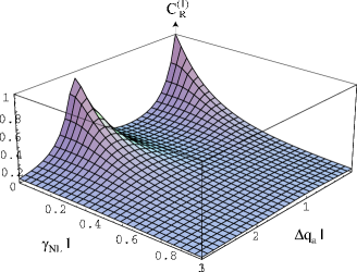
(b)

Figure 2: (a) Short-range angular correlation function of the fluctuations of diffusely reflected intensity in a semi-infinite nonlinear disordered medium. (b) Line shape of the coherent backscattering cone in a semi-infinite nonlinear disordered medium for $L_{\mathrm{a}}^{\mathrm{NL}}\rightarrow\infty$ [vanishing linear and nonlinear absorption, curve (a)] and $L_{\mathrm{a}}^{\mathrm{NL}}=10\ell$ [curve (b)]. The figures are from Ref. [17].

Finally, the coherent backscattering cone can be calculated at the same level of approximation bressoux00 . If the nonlinear coefficient $\varepsilon_{2}$ in Eq. (1) is purely real, no deviation from the linear result (9) is found within the present theoretical framework. The contribution of the crossed diagrams to the intensity of backscattered wave is, however, modified if $\varepsilon_{2}$ has a small imaginary part (i.e. in the presence of nonlinear absorption). This phenomenon can be described by introducing a generalized absorption length $L_{\mathrm{a}}^{\mathrm{NL}}$, accounting for both linear and nonlinear absorption:

$$\frac{1}{(L_{\mathrm{a}}^{\mathrm{NL}})^{2}}\approx\frac{1}{L_{\mathrm{a}}^{2}}+\frac{k_{0}}{\ell}(1+\zeta)A^{2}{\mathrm{Im}}\varepsilon_{2}.$$ (22)

Additional absorption, introduced by the nonlinear term in Eq. (1), will lead to the rounding of the triangular peak shape of the coherent backscattering cone, as illustrated in Fig. 2(b). Mathematically, this phenomenon is described by Eq. (9) with $L_{\mathrm{a}}$ replaced by $L_{\mathrm{a}}^{\mathrm{NL}}$.

To conclude this section, we would like to emphasize that in calculating the angular correlation functions [Eqs. (19), (21) and Figs. 1(b), 2(a)] and the coherent backscattering cone [Fig. 2(b)], we have completely neglected the fluctuations of the wave intensity inside the disordered medium, replacing $I({\mathbf{r}})$ by $\left<I({\mathbf{r}})\right>\approx A^{2}=\mathrm{const}$ in the very beginning [Eq. (16)]. The intensity fluctuations in disordered media are, however, known to be important and exhibit some nontrivial features [such as, e.g., long-range correlations, see Eq. (4)]. It is therefore important to analyze the role of these fluctuations in the presence of nonlinearity, when the highly irregular spatial intensity distribution (speckle pattern) can give rise to a random modification of the dielectric constant (and, consequently, refractive index). Such an analysis is presented in the following section.

V Instability of Diffuse Waves in Nonlinear Disordered Media

As we already mentioned in Sec. III, unstable regimes are encountered in many nonlinear optical systems. It is therefore natural to expect that they may appear in a disordered nonlinear medium as well. The origin of the instability in this case is relatively easy to understand in the framework of the path-integral picture of wave propagation skip00 .

V.1 Heuristic description

In the path-integral picture, the diffusely scattered wave field at some position ${\mathbf{r}}$ inside the disordered medium is represented as a sum of partial waves traveling along various diffuse paths. Due to the nonlinearity of the medium, the phase $\phi({\mathbf{r}},t)$ of a given partial wave arriving at ${\mathbf{r}}$ at time $t$ depends on the spatio-temporal distribution of intensity $I({\mathbf{r}},t)$ (speckle pattern) inside the medium. At the same time, $I({\mathbf{r}},t)$ is a result of interference of many partial waves, and, therefore, $I({\mathbf{r}},t)$ is sensitive to their phases $\phi({\mathbf{r}},t)$. This leads to a sort of feedback mechanism: The phases of partial waves depend on the speckle pattern $I({\mathbf{r}},t)$, while the latter depends on the phases. It appears that such a feedback can destabilize the time-independent speckle pattern $I({\mathbf{r}})$, leading to $I({\mathbf{r}},t)$ that fluctuates spontaneously with time, if the nonlinearity is strong enough skip00 . As we show below, this phenomenon can be understood in reasonably simple terms in the case of local ($a_{\mathrm{NL}}=0$) and instantaneous ($\tau_{\mathrm{NL}}=0$) Kerr nonlinearity.

Consider a partial wave traveling along a typical diffuse path of length $s_{0}(t)\sim L^{2}/\ell$ from the source of waves to some point ${\mathbf{r}}$ located at a distance $L$ from the source. We assume that the path length $s_{0}(t)$ can vary slowly with time due to, e.g., the motion of scattering centers [corresponding to a time-dependent disorder $\delta\varepsilon({\mathbf{r}},t)$ in Eq. (1)], while the initial and final points of the path are fixed. The variations of $s_{0}$ with time are assumed to be slow (i.e. $s_{0}$ does not change significantly during the time $T_{\mathrm{D}}=L^{2}/D$ required for the wave to cover the distance of order $s_{0}$). The phase $\phi({\mathbf{r}},t)$ of the wave contains a ‘linear’ contribution $\phi_{\mathrm{L}}({\mathbf{r}},t)=k_{0}s_{0}(t)$ and the ‘nonlinear’ one

$$\phi_{\mathrm{NL}}({\mathbf{r}},t) = k_{0}\int_{0}^{s_{0}(t)}ds_{1}[\Delta\varepsilon_{\mathrm{NL}}({\mathbf{r}}_{1},t_{1})/2]$$ (23)

$$= k_{0}n_{2}\int_{0}^{s_{0}(t)}ds_{1}I({\mathbf{r}}_{1},t_{1}),$$

where $\Delta\varepsilon_{\mathrm{NL}}({\mathbf{r}}_{1},t_{1})/2=n_{2}I({\mathbf{r}}_{1},t_{1})$ is the nonlinear part of the refractive index, $s_{1}$ is a curvilinear coordinate of the point ${\mathbf{r}}_{1}$ along the path, $t_{1}=t-[s_{0}(t)-s_{1}]/c$ is the time of wave passage through ${\mathbf{r}}_{1}$, and the integrals are along the path.

Let the fluctuating part of the linear dielectric constant $\delta\varepsilon({\mathbf{r}},t)$ to change slightly during some time interval $\Delta t$: $\delta\varepsilon({\mathbf{r}},t)\rightarrow\delta\varepsilon({\mathbf{r}},t+\Delta t)=\delta\varepsilon({\mathbf{r}},t)+\Delta[\delta\varepsilon({\mathbf{r}},t)]$, leading to corresponding changes $\Delta I({\mathbf{r}},t,\Delta t)$ and $\Delta\phi({\mathbf{r}},t,\Delta t)$ of intensity and phase, respectively. The latter can be, in principle, found from Eq. (1). $\Delta\phi$ contains the linear and nonlinear parts, $\Delta\phi_{\mathrm{L}}$ and $\Delta\phi_{\mathrm{NL}}$, respectively. Under very general assumptions, one can show that $\left<\Delta I\right>=0$ and $\left<\Delta\phi\right>=0$, where the averaging is over $\delta\varepsilon({\mathbf{r}},t)$, $\Delta[\delta\varepsilon({\mathbf{r}},t)]$, and over all paths of the same length $s_{0}$. The second moment $\left<\Delta\phi^{2}\right>=\left<\Delta\phi_{\mathrm{L}}^{2}\right>+\left<\Delta\phi_{\mathrm{NL}}^{2}\right>>0$, where $\left<\Delta\phi_{\mathrm{L}}^{2}\right>$ is calculated in the framework of the so-called diffusing-wave spectroscopy (DWS) maret87 and depends on the way in which $\delta\varepsilon({\mathbf{r}},t)$ is modified. If, for example, the disordered medium is a suspension of Brownian particles (particle diffusion coefficient $D_{\mathrm{B}}$), $\left<\Delta\phi_{\mathrm{L}}^{2}\right>=(\Delta t/\tau_{0})(s_{0}/\ell)$, where $\tau_{0}=(4k_{0}^{2}D_{\mathrm{B}})^{-1}$ maret87 . For the variance of the nonlinear phase difference, Eq. (23) yields

$$\left<\Delta\phi_{\mathrm{NL}}^{2}\right>=k_{0}^{2}n_{2}^{2}\int_{0}^{s_{0}}ds_{1}\int_{0}^{s_{0}}ds_{2}$$

$$\hskip 28.45274pt\left<\Delta I({\mathbf{r}}_{1},t_{1})\Delta I({\mathbf{r}}_{2},t_{2})\right>,$$ (24)

where $t_{2}=t_{1}+\Delta t$ and both integrals are along the same diffusion path. Obviously,

$$\left<\Delta I({\mathbf{r}}_{1},t_{1})\Delta I({\mathbf{r}}_{2},t_{2})\right>=2\left[\left<\delta I({\mathbf{r}}_{1},t)\delta I({\mathbf{r}}_{2},t)\right>\right.$$

$$\hskip 28.45274pt-\left.\left<\delta I({\mathbf{r}}_{1},t)\delta I({\mathbf{r}}_{2},t+\Delta t)\right>\right]$$

$$\hskip 28.45274pt\simeq\left<\Delta\phi_{\mathrm{L}}^{2}\right>\left<\delta I({\mathbf{r}}_{1},t)\delta I({\mathbf{r}}_{2},t)\right>,$$ (25)

where the second line is obtained by assuming that $\left<\delta I({\mathbf{r}}_{1},t)\delta I({\mathbf{r}}_{2},t+\Delta t)\right>$ in the nonlinear medium is close to its value in the linear one (a sort of perturbation theory), replacing $\left<\delta I({\mathbf{r}}_{1},t)\delta I({\mathbf{r}}_{2},t+\Delta t)\right>$ by the ‘linear’ result:

$$\left<\delta I({\mathbf{r}}_{1},t)\delta I({\mathbf{r}}_{2},t+\Delta t)\right>\simeq\left<\delta I({\mathbf{r}}_{1},t)\delta I({\mathbf{r}}_{2},t)\right>$$

$$\hskip 28.45274pt=\exp\left[-(1/2)\left<\Delta\phi_{\mathrm{L}}^{2}\right>\right],$$ (26)

and assuming $\left<\Delta\phi_{\mathrm{L}}^{2}\right>\ll 1$.

Substituting Eq. (25) into Eq. (24) and changing the variables of integration to $s=(s_{1}+s_{2})/2$ and $\Delta s=s_{1}-s_{2}$, we obtain

$$\left<\Delta\phi_{\mathrm{NL}}^{2}\right>=\left<\Delta\phi_{\mathrm{L}}^{2}\right>k_{0}^{2}n_{2}^{2}\int_{0}^{s_{0}}ds\int_{-s}^{s}d\Delta s\left<\delta I({\mathbf{r}}_{1})\delta I({\mathbf{r}}_{2})\right>.$$

(27)

As we discussed in Sec. II, the correlation function of intensity fluctuations $\left<\delta I({\mathbf{r}}_{1})\delta I({\mathbf{r}}_{2})\right>$ in Eq. (27) contains two contributions: a short-range one [Eq. (3)] and a long-range one [Eq. (4)]. To perform the integration in Eq. (27), we replace $\Delta r=\left|{\mathbf{r}}_{1}-{\mathbf{r}}_{2}\right|$ in the expression (3) for the short-range correlation function by $\Delta s$, assuming the wave path to be ballistic at distances shorter than $\ell$. In contrast, for $\Delta r>\ell$ the wave path is diffusive, and hence $\Delta r$ in the expression (4) for the long-range correlation function can be substituted by $(\Delta s\ell)^{1/2}$. Performing then integrations in Eq. (27) yields

$$\left<\Delta\phi_{\mathrm{NL}}^{2}\right>\simeq p\left<\Delta\phi_{\mathrm{L}}^{2}\right>,$$ (28)

where we introduce the bifurcation parameter skip00

$$p=\Delta n^{2}\left(\frac{L}{\ell}\right)^{2}\left(k_{0}\ell+\frac{L}{\ell}\right),$$ (29)

and the numerical factors of order unity are omitted.

Note that Eq. (29) is a sum of two contributions. The first one, $\Delta n^{2}$ $(L/\ell)^{2}k_{0}\ell$, originates from the short-range correlation of intensity fluctuations [Eq. (3)], while the second contribution, $\Delta n^{2}(L/\ell)^{3}$, is due to the long-range correlation [Eq. (4)]. If $p\ll 1$, the nonlinear term $\left<\Delta\phi_{\mathrm{NL}}^{2}\right>$ represents just a small correction to the linear one $\left<\Delta\phi_{\mathrm{L}}^{2}\right>$ and our perturbation approach is likely to be valid. In contrast, the above perturbation theory diverges for $p>1$, since $\left<\Delta\phi_{\mathrm{NL}}^{2}\right>$ becomes larger than $\left<\Delta\phi_{\mathrm{L}}^{2}\right>$. This suggests that $p\simeq 1$ is a critical point beyond which (i.e. for $p>1$) the physics of the nonlinear problem is no longer similar to the physics of the linear one and hence the perturbation theory cannot be used. Although the mere breakdown of the perturbation theory does not permit to draw any far-reaching conclusions about the speckle pattern beyond the critical point $p\simeq 1$, a more rigorous analysis (see Secs. V.2 and V.3) shows that $p\simeq 1$ defines the instability threshold of the multiple-scattering speckle pattern, and that at $p>1$ the latter should exhibit spontaneous temporal fluctuations even for a time-independent disorder $\delta\varepsilon({\mathbf{r}})$ (i.e. for vanishing mobility of scattering centers: $D_{\mathrm{B}}\rightarrow 0$ and $\tau_{0}\rightarrow\infty$ in the case of Brownian motion).

It is pertinent to note the extensive nature of the bifurcation parameter $p$. According to Eq. (29), weak nonlinearity can be efficiently compensated by a sufficiently large sample size $L$ and $p\sim 1$ can be reached even at vanishing $\Delta n$, provided that $L$ is large enough. In the limit of large sample size $L\gg k_{0}\ell^{2}$, one gets $p\simeq\Delta n^{2}(L/\ell)^{3}$ (as also found in Ref. spivak00 ). This result is due to the long-range correlation (4) of intensity fluctuations which dominates in the integral of Eq. (27) because of its slow decrease ($\propto\left|{\mathbf{r}}_{1}-{\mathbf{r}}_{2}\right|^{-1}$) and consequent extension over the whole disordered sample. Another remarkable feature of Eq. (29) is the independence of $p$ of the sign of $\Delta n$. The phenomenon of the speckle pattern instability is therefore expected to develop in a similar way for both positive and negative nonlinear coefficients $n_{2}$. This is not common for the instabilities in nonlinear systems without disorder ikeda80 –soljacic00 since the latter are often related to the self-focusing effect, arising at $n_{2}>0$ only. The instability discussed in the present paper is of different type and has nothing to do with the self-focusing [which is negligible if the condition (14) is satisfied]. This does not mean, however, that the phenomena similar to those discussed in the present paper do not exist in homogeneous nonlinear media. In fact, it is easy to see that Eq. (23) describes nothing but the self-phase modulation boyd02 of the multiple-scattering speckle pattern. It is worth noting that the development of the self-phase modulation in a disordered medium appears to be rather different from that in the homogeneous case. Indeed, in a homogeneous medium of size $L$ the nonlinear phase shift is deterministic and $\phi_{\mathrm{NL}}=k_{0}n_{2}I_{0}L$ for a wave of intensity $I_{0}$, while in the case of diffuse multiple scattering $\phi_{\mathrm{NL}}$ is random with the average value $\left<\phi_{\mathrm{NL}}\right>\simeq k_{0}n_{2}I_{0}(L^{2}/\ell)$ and variance $\left<\phi_{\mathrm{NL}}^{2}\right>-\left<\phi_{\mathrm{NL}}\right>^{2}\simeq p$. The threshold of the speckle pattern instability $p\simeq 1$ is then simply the point where the sample-to-sample fluctuations of the nonlinear phase shift become of order unity.

To conclude this subsection, we would like to comment on the recent results on modulation instability (MI) of incoherent light beams in homogeneous nonlinear media soljacic00 . In this case, a 2D speckle pattern (speckled beam) with a controlled degree of spatial and temporal coherence is ‘prepared’ by sending a coherent laser beam on a rotating diffuser. The beam is then incident on a homogeneous nonlinear medium (inorganic photorefractive crystal). Pattern formation and ‘optical turbulence’ is observed if the intensity of the beam exceeds a specific threshold, determined by the degree of coherence of the beam (coherent MI has no threshold). Although the study presented in this paper is also concerned with the instability of speckle patterns in nonlinear media, it differs essentially from that of Ref. soljacic00 at least in the following important aspects: (a) the initially coherent wave loses its spatial coherence inside the medium, due to the multiple scattering on heterogeneities of the refractive index, (b) the temporal coherence of the incident light is perfect (in the case of incoherent MI soljacic00 , the coherence time of the incident beam is much shorter than the response time of the medium $\tau_{\mathrm{NL}}$), and (c) the incident light beam is completely destroyed by the scattering after a distance $\sim\ell$ and light propagation is diffusive in the bulk of the sample. In addition, diffuse multiple scattering of light results in a distributed feedback mechanism, absent in the case of MI.

V.2 Path-Integral Picture

A mathematically rigorous formulation of the heuristic analysis presented in the previous subsection has been performed in Ref. skip00 . In addition to the condition of weak nonlinearity (14) we anticipate that the expected spontaneous fluctuations of the speckle pattern beyond the instability threshold will be slow enough or, more precisely, that the typical time of the speckle pattern dynamics will be much longer than the typical time between two successive scattering events $\ell/c$.

For the sake of the mathematical simplicity, we consider a plane monochromatic wave incident on the stationary [$\delta\varepsilon({\mathbf{r}})$ is time-independent] semi-infinite disordered medium ($L\rightarrow\infty$) with a finite (macroscopic) absorption length $L_{\mathrm{a}}\gg\ell$ and a local ($a_{\mathrm{NL}}=0$) instantaneous ($\tau_{\mathrm{NL}}=0$) Kerr nonlinearity. It appears that instead of replacing the intensity correlation function $\left<\delta I({\mathbf{r}}_{1},t)\delta I({\mathbf{r}}_{2},t+\Delta t)\right>$ in Eq. (25) by its ‘linear’ value (and thus constructing a sort of perturbation theory), one can obtain a self-consistent description of the speckle instability. The analysis skip00 leads to a self-consistent equation for $\beta=-\ln g_{1}$, where $g_{1}(\tau)=\left<E(t)E^{*}(t+\tau)\right>/\left<\left|E(t)\right|^{2}\right>$ is the time autocorrelation function of diffusely reflected wave, and $g_{1}$ denotes $\lim_{\tau\rightarrow\infty}g_{1}(\tau)$:

$$\exp\left(-\beta\right)=F\left(\beta\right),$$ (30)

where $F(\beta)$ is a known monotonically decaying function and $F(0)=1$.

Figure 3: (a) Graphical solution of Eq. (30) at $k_{0}\ell=100$, $\left|\Delta n\right|=10^{-4}$ and the values of $\ell/L_{\mathrm{a}}$ indicated near each curve. The solid lines show $F(\beta)$, the dashed line is $\exp(-\beta)$. Thick solid lines with arrows illustrate the iterative solution of Eq. (30). (b) Bifurcation diagram of the speckle pattern in a semi-infinite disordered medium for $k_{0}\ell=100$ and the values of $\ell/L_{\mathrm{a}}$ indicated near the each curve. The threshold values of $\left|\Delta n\right|$, following from the condition $p=1$ at $\ell/L_{\mathrm{a}}>0$, are indicated by arrows. In the absence of absorption, $\ell/L_{\mathrm{a}}=0$ (dashed line), there is no threshold and the speckle pattern is unstable at any (even infinitely small !) $\left|\Delta n\right|$. The figures are from Ref. [16].

Fig. 3(a) illustrates the graphical solution of Eq. (30) for some realistic values of parameters. At strong enough absorption [two upper curves in Fig. 3(a)], a unique solution $\beta=\beta_{1}=0$ exists, corresponding to $g_{1}=\exp(-\beta)=1$. This means that the time autocorrelation function of diffusely reflected wave $g_{1}(\tau)$ does not decay with time, remaining equal to $1$ for all $\tau$ (even for $\tau\rightarrow\infty$). The speckle pattern is therefore stationary (i.e. does not change with time). In contrast, for weak absorption [three lower curves in Fig. 3(a)] a second solution $\beta=\beta_{2}>0$ arises, corresponding to $g_{1}=\exp(-\beta)<1$. Eq. (30) now has two fixed points: $\beta=\beta_{1}=0$ and $\beta=\beta_{2}>0$. It is seen from Fig. 3(a) (see thick solid lines with arrows) that an iterative solution of Eq. (30) starting at some $\beta>0$ converges to $\beta=\beta_{1}=0$ for strong enough absorption and to $\beta=\beta_{2}>0$ for weak absorption. $\beta=\beta_{2}>0$ is therefore a stationary point of Eq. (30) in the latter case, corresponding to the physically realizable solution beyond the instability threshold. $\beta>0$ and $g_{1}<1$ signifies that the time autocorrelation function of diffusely reflected wave $g_{1}(\tau)$ decays with $\tau$ despite our assumption of stationary disorder [time-independent $\delta\varepsilon({\mathbf{r}})$], although the present analysis does not allow us to estimate the characteristic time scale of this decrease. Decaying $g_{1}(\tau)$ corresponds to an unstable (i.e. time-varying) speckle pattern. Note that in contrast to the fluctuations of the speckle pattern due to the motion of scattering centers, employed in DWS to study the dynamics of the medium maret87 , the speckle dynamics in a stationary nonlinear random medium is spontaneous, i.e. it does not originate from the motion of scattering centers (since the latter are immobile) but is intrinsic for the underlying nonlinear wave equation (1). Spontaneous speckle dynamics is irreversible and hence the instability threshold $p\simeq 1$ is the point where the time-reversal symmetry is spontaneously broken for the multiple-scattered waves.

Fig. 3(b) shows the time autocorrelation function $g_{1}=\exp(-\beta)$ obtained by solving Eq. (30) at $k_{0}\ell=100$ and several values of $\ell/L_{\mathrm{a}}$. The transition from the stable ($g_{1}=1$) to unstable ($g_{1}<1$) regime is clearly seen when $\ell/L_{\mathrm{a}}>0$. At $\ell/L_{\mathrm{a}}=0$ (no absorption), we find that $g_{1}<1$ at any, even infinitely small $\left|\Delta n\right|$. The border between stable ($g_{1}=1$) and unstable ($g_{1}<1$) regimes can be found analytically by requiring $(\partial/\partial\beta)F(\beta)=-1$ at $\beta=0$. This yields $p\simeq 1$ as the instability threshold, where the bifurcation parameter $p$ is defined by Eq. (29) with $L$ replaced by $L_{\mathrm{a}}$. The threshold values of $\left|\Delta n\right|$ following from the condition $p=1$ are shown in Fig. 3(b) by arrows.

V.3 Langevin Description

Although the path-integral approach, sketched in the two previous subsections, allows us to predict the instability of the multiple-scattering speckle pattern in a nonlinear disordered medium and even to calculate $g_{1}(\tau)$ in the limit $\tau\rightarrow\infty$, it does not permit to estimate the time scale of spontaneous intensity fluctuations beyond the instability threshold. Meanwhile, this issue is of primary importance in view of the possible experimental observation of the instability phenomenon. In this subsection, we show that the spontaneous speckle dynamics can be studied by using the Langevin approach skip02a ; skip02b .

As in the previous subsections, we assume the nonlinearity to be local ($a_{\mathrm{NL}}=0$), but consider arbitrary nonlinearity response time $\tau_{\mathrm{NL}}$. The nonlinear part of the dielectric constant is assumed to be governed by Eq. (10). In addition, we neglect the absorption (assuming $L_{\mathrm{a}}\gg L$) and restrict our consideration to the case when the development of the speckle pattern instability is dominated by the long-range intensity correlations. This requires the sample size to be large enough [$L\gg k_{0}\ell^{2}$, see Eq. (29) and its accompanying discussion] and the speckle dynamics to be slow (time scale of spontaneous intensity fluctuations $\tau\gg T_{\mathrm{D}}[(k_{0}\ell^{2})/L]^{2}$). The latter condition follows from Eq. (27), where the limits of integration over $\Delta s$ should be set to $\mp c\tau$, if $c\tau\ll s_{0}$ (or, equivalently, $\tau\ll T_{\mathrm{D}}$), since the correlation has simply no time to establish beyond these limits due to the finite speed of wave propagation. Integration in Eq. (27) then yields

$$\left<\Delta\phi_{\mathrm{NL}}^{2}\right>\simeq\Delta n^{2}\left(\frac{L}{\ell}\right)^{2}\left[k_{0}\ell+\frac{L}{\ell}\left(\frac{\tau}{T_{\mathrm{D}}}\right)^{1/2}\right]\left<\Delta\phi_{\mathrm{L}}^{2}\right>,$$

(31)

where the first term in square brackets [the same as in Eq. (29)] results from the short-range correlation (3), while the second term is due to the long-range one (4). Requiring that the second term dominates the first, we obtain $\tau\gg T_{\mathrm{D}}[(k_{0}\ell^{2})/L]^{2}$ as stated above.

The Langevin equation for the intensity fluctuation $\delta I({\mathbf{r}},t)$ reads zyuzin87 :

$$\frac{\partial}{\partial t}\delta I({\mathbf{r}},t)-D\nabla^{2}\delta I({\mathbf{r}},t)=-{\mathbf{\nabla}}\cdot{{\mathbf{j}}}_{\mathrm{ext}}({\mathbf{r}},t),$$ (32)

where ${{\mathbf{j}}}_{\mathrm{ext}}({\mathbf{r}},t)$ are random external Langevin currents that have zero mean and a correlation function $\left<j_{\mathrm{ext}}^{(i)}({\mathbf{r}},t)j_{\mathrm{ext}}^{(j)}({\mathbf{r}}_{1},t_{1})\right>$ given by the diagram (i) of Fig. 4(a). Being a ‘fingerprint’ of disorder, the Langevin currents will be modified if we modify the dielectric constant of the medium. In our case, the linear part of the dielectric constant is fixed [$\delta\varepsilon({\mathbf{r}})$ in Eq. (1) is time-independent], but its nonlinear part $\Delta\varepsilon_{\mathrm{NL}}({\mathbf{r}},t)$ can vary with time, and it is relatively easy to obtain the following dynamic equation for ${\mathbf{j}}_{\mathrm{ext}}({\mathbf{r}},t)$ skip02a ; skip02b :

$$\frac{\partial}{\partial t}{\mathbf{j}}_{\mathrm{ext}}({\mathbf{r}},t)=\int_{V}d^{3}{\mathbf{r}}^{\,\prime}\int_{0}^{\infty}d\Delta t\,$$

$${\mathbf{q}}({\mathbf{r}},{\mathbf{r}}^{\,\prime},\Delta t)\;\frac{\partial}{\partial t}\Delta\varepsilon_{\mathrm{NL}}({\mathbf{r}}^{\,\prime},t-\Delta t),$$ (33)

where ${\mathbf{q}}({\mathbf{r}},{\mathbf{r}}^{\,\prime},\Delta t)$ is a random response function with zero mean and the correlation function $\left<q^{(i)}({\mathbf{r}},{\mathbf{r}}^{\,\prime},\Delta t)q^{(j)*}({\mathbf{r}}_{1},{\mathbf{r}}_{1}^{\,\prime},\Delta t_{1})\right>$ given by a sum of the diagrams (ii) and (iii) of Fig. 4(a). Eqs. (32) and (33) together with Eq. (10) for $\Delta\varepsilon_{\mathrm{NL}}$ form a self-consistent system of equations for the stability analysis of the speckle pattern.

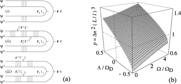
Figure 4: (a) Diagrams contributing to the correlation functions of Langevin currents ${\mathbf{j}}_{\mathrm{ext}}({\mathbf{r}},t)$ [diagram (i)] and random response functions ${\mathbf{q}}({\mathbf{r}},{\mathbf{r}}^{\,\prime},\Delta t)$ [diagrams (ii) and (iii)]. The diagrams (ii) and (iii) are obtained by the functional differentiation of the diagram (i) with respect to the dielectric constant of the disordered medium. Wavy lines in the diagrams (ii) and (iii) denote $k_{0}^{2}$ factors. (b) Surface describing the stability of the multiple-scattering speckle pattern in a disordered medium with fast nonlinearity ($\Omega_{\mathrm{D}}\tau_{\mathrm{NL}}\ll 1$). For given frequency $\Omega$ and bifurcation parameter $p$, the surface shown in the figure allows one to determine the value of the Lyapunov exponent $\Lambda$. If $\Lambda>0$, the speckle pattern is unstable with respect to excitations at frequency $\Omega$. The figures are from Ref. [18].

Consider now an infinitesimal periodic excitation of the stationary speckle pattern: $\delta I({\mathbf{r}},t)=\delta I({\mathbf{r}},\alpha)$ $\exp(\alpha t)$, where $\alpha=i\Omega+\Lambda\neq 0$ and $\Omega>0$. Such an excitation can be either damped or amplified, depending on the sign of the Lyapunov exponent $\Lambda$. The value of $\Lambda$ is determined by two competing processes: on the one hand, diffusion tends to smear the excitation out, while on the other hand, the distributed feedback sustains its existence. The mathematical description of this competition is provided by Eqs. (32), (33), and (10) that after the substitution of $\delta I({\mathbf{r}},t)=\delta I({\mathbf{r}},\alpha)\exp(i\alpha t)$ [and similarly for ${\mathbf{j}}_{\mathrm{ext}}({\mathbf{r}},t)$ and $\Delta\varepsilon_{\mathrm{NL}}({\mathbf{r}},t)$] lead to the following equation for $p$, $\Omega$, and $\Lambda$ skip02a ; skip02b :

$$p\simeq F_{1}\left(\Omega/\Omega_{\mathrm{D}},\Lambda/\Omega_{\mathrm{D}}\right)F_{2}\left(\Omega\tau_{\mathrm{NL}},\Lambda\tau_{\mathrm{NL}}\right),$$ (34)

where $\Omega_{\mathrm{D}}=1/T_{\mathrm{D}}=D/L^{2}$ and the function $F_{1}$ is shown in Fig. 4(b) for the case of the sample with open boundaries, while $F_{2}(x,y)=1+x^{2}+y^{2}+2y$.

Let us first consider the fast nonlinearity, assuming $\tau_{\mathrm{NL}}\Omega_{\mathrm{D}}\ll 1$ skip02a . In this case, the nonlinear response takes much less time than the typical perturbation $\delta I({\mathbf{r}},\alpha)$ needs to extend throughout the disordered sample and we can set $F_{2}\left(\Omega\tau_{\mathrm{NL}},\Lambda\tau_{\mathrm{NL}}\right)\simeq 1$ in Eq. (34). The stability of the speckle pattern with respect to periodic excitations is then described by Fig. 4(b). For a given frequency $\Omega$, the sign of the Lyapunov exponent $\Lambda$ depends on the value of $p$. Excitations at frequencies $\Omega$ corresponding to $\Lambda<0$ are damped exponentially and thus soon disappear. In contrast, excitations at frequencies $\Omega$ corresponding to $\Lambda>0$ are exponentially amplified, which signifies the instability of the speckle pattern with respect to excitations at such frequencies. Noting that $\Lambda$ is always negative for $p<1$, we conclude that all excitation are damped in this case and the speckle pattern is absolutely stable. In an experiment, any spontaneous excitation of the static speckle pattern will be suppressed and the speckle pattern will be independent of time: $\delta I({\mathbf{r}},t)=\delta I({\mathbf{r}})$, as in the linear case. When $p>1$, an interval of frequencies $0<\Omega<\Omega_{\mathrm{max}}$ starts to open up with $\Lambda>0$. The speckle pattern thus becomes unstable with respect to excitations at low frequencies. In an experiment, any spontaneous excitation of the static speckle pattern at frequency $\Omega\in(0,\Omega_{\mathrm{max}})$ will be amplified and one will observe a time-varying speckle pattern $\delta I({\mathbf{r}},t)$. Note that the absolute instability threshold $p\simeq 1$ agrees with the results of Secs. V.1 and V.2, while completely different calculation techniques have been applied in the three cases.

Figure 5: (a) Frequency-dependent instability threshold for a disordered sample with instantaneous nonlinear response and open boundaries. The inset shows the maximal Lyapunov exponent as a function of the bifurcation parameter $p$. (b) The same as (a) but for a sample with a nonzero nonlinearity response time $\tau_{\mathrm{NL}}$. The dashed line shows the result corresponding to $\tau_{\mathrm{NL}}\Omega_{\mathrm{D}}=0$ [the same as the solid line in the panel (a)]. The figures are from Ref. [18] (a) and [19] (b).

Fig. 5(a) shows the frequency-dependent instability threshold for the disordered sample with open boundaries and fast nonlinear response. Detailed analysis skip02a of Eq. (34) shows that the frequency-dependent threshold value of $p$ scales as $1+C_{1}(\Omega/\Omega_{\mathrm{D}})^{2}$ (where $C_{1}\sim 1$ is a numerical constant) at $\Omega\ll\Omega_{\mathrm{D}}$ and as $(\Omega/\Omega_{\mathrm{D}})^{1/2}$ at $\Omega\gg\Omega_{\mathrm{D}}$. The latter result can also be obtained from Eq. (31) by setting $\tau\sim 1/\Omega$ and applying $\left<\Delta\phi_{\mathrm{NL}}^{2}\right>>\left<\Delta\phi_{\mathrm{L}}^{2}\right>$ as the instability condition. For a given value of $p>1$, the maximum excited frequency is $\Omega_{\mathrm{max}}\sim\Omega_{\mathrm{D}}(p-1)^{1/2}$ for $p-1\ll 1$ and $\Omega_{\mathrm{max}}\sim\Omega_{\mathrm{D}}p^{2}$ for $p-1>1$.

Fig. 5(b) illustrates the effect of noninstantaneous nonlinearity on the frequency-dependent instability threshold for several values of $\tau_{\mathrm{NL}}\Omega_{\mathrm{D}}$ skip02b . Obviously, slow nonlinear response of the medium rises the instability threshold for high-frequency excitations, while the absolute instability threshold $p\simeq 1$ remains the same, independent of the nonlinearity response time $\tau_{\mathrm{NL}}$. The reason for this is that just above $p=1$ the speckle pattern becomes unstable with respect to excitations at very low frequencies, for which $\Omega\ll 1/\tau_{\mathrm{NL}}$ is always fulfilled and which, therefore, are not sensitive to the value of $\tau_{\mathrm{NL}}$ [mathematically, $F_{2}(\Omega\tau_{\mathrm{NL}},\Lambda\tau_{\mathrm{NL}})\simeq 1$ in Eq. (34)]. In the limit of slow nonlinearity ($\tau_{\mathrm{NL}}\Omega_{\mathrm{D}}\gg 1$) and for $1<p-1\ll 1$ we can set $F_{1}\left(\Omega/\Omega_{\mathrm{D}},\Lambda/\Omega_{\mathrm{D}}\right)\simeq 1$ in Eq. (34) and find the threshold value of $p$ to scale as $1+(\Omega\tau_{\mathrm{NL}})^{2}$ and $\Omega_{\mathrm{max}}\sim\tau_{\mathrm{NL}}^{-1}(p-1)^{1/2}$.

As follows from the above analysis, a continuous low-frequency spectrum of frequencies $(0,\Omega_{\mathrm{max}})$ is excited at $p>1$. In addition, the Lyapunov exponent $\Lambda$ appears to decrease monotonically with $\Omega$, favoring no specific frequency $\Omega$ just above the threshold skip02b . This allows us to hypothesize that at $p=1$ the speckle pattern undergoes a transition from a stationary to chaotic state. Such a behavior should be contrasted from the ‘route to chaos’ through a sequence of bifurcations, characteristic of many nonlinear and, in particular, optical systems ikeda80 –voron99 .

VI Conclusion

The present paper reviews some of the recent theoretical developments in the field of multiple wave scattering in nonlinear disordered media. To be specific, we consider optical waves and restrict ourselves to the case of Kerr nonlinearity. Assuming that the nonlinearity is weak, we derive the expressions for the angular correlation functions and the coherent backscattering cone in a nonlinear disordered medium (Sec. IV). In both transmission and reflection, the short-range angular correlation functions of intensity fluctuations for two waves with different amplitudes ($A$ and $A^{\prime}\rightarrow 0$) appear to be given by the same expressions [Eqs. (6) and (7), respectively] as the angular correlation functions for waves at two different frequencies ($\omega$ and $\omega^{\prime}=\omega-\Delta\omega$) in a linear medium, with $\Delta\omega$ replaced by $2\ell c/(3\xi^{2})$, where $\xi$ is a new nonlinear characteristic length defined by Eq. (20). The coherent backscattering cone is not affected by the nonlinearity, as long as the nonlinear coefficient $\varepsilon_{2}$ in Eq. (1) is purely real. If $\varepsilon_{2}$ has an imaginary part (which corresponds to the nonlinear absorption), the line shape of the cone is given by the same expression (9) as in an absorbing linear medium, where the linear macroscopic absorption length $L_{\mathrm{a}}$ should be replaced by the generalized absorption length $L_{\mathrm{a}}^{\mathrm{NL}}$ defined by Eq. (22).

For the nonlinearity strength exceeding a threshold $p\simeq 1$ [with the bifurcation parameter $p$ given by Eq. (29)], we predict a new phenomenon — temporal instability of the multiple-scattering speckle pattern — to take place (Sec. V). The instability is due to a combined effect of the nonlinear self-phase modulation and the distributed feedback mechanism provided by multiple scattering and should manifest itself in spontaneous fluctuations of the speckle pattern with time. Since the spontaneous dynamics of the speckle pattern is irreversible, the time-reversal symmetry is spontaneously broken when $p$ surpasses 1. The important feature of our result is the extensive nature of the instability threshold, leading to an interesting possibility of obtaining unstable regimes even at very weak nonlinearities, provided that the disordered sample is large enough. To study the dynamics of multiple-scattering speckle patterns beyond the instability threshold, we generalize the Langevin description of wave diffusion in disordered media (Sec. V.3). Explicit expressions for the characteristic time scale of spontaneous intensity fluctuations are derived with account for the noninstantaneous nature of the nonlinearity. The results of this study allow us to hypothesize that the dynamics of the speckle pattern may become chaotic immediately beyond the instability threshold, and that the cascade of bifurcations, typical for chaotic transitions in many known nonlinear systems ikeda80 –voron99 , might not be present in the considered case of diffuse waves.

Finally, we discuss the experimental implications of our results. With common nonlinear materials, such as, e.g., carbon disulfide, $n_{2}\simeq 3\times 10^{-14}$ cm²/W can be realized boyd02 . At $I\simeq 1$ MW/cm² this yields $\Delta n\simeq 3\times 10^{-8}$ and the characteristic length $\xi$ defined in Eq. (20) is $\xi\simeq 2$ cm for $\ell\simeq 100$ $\mu$m and $\lambda\simeq 0.5$ $\mu$m. As follows from Eq. (19), $\xi\lesssim L$ is required to observe a sizeable effect of the nonlinearity on the angular correlation function of transmitted light, and hence using a 2 cm-thick disordered sample should suffice to make the effect of nonlinearity measurable in, e.g., a dense suspension of carbon disulfide particles. In contrast, $\xi\lesssim\ell$ is necessary to observe the effect of the nonlinearity on the angular correlation function in the reflection geometry. This requires a stronger nonlinearity. In nematic liquid crystals, for example, $\Delta n$ up to $0.1$ is achievable (see, e.g., Ref. muenster97 ). Taking $\Delta n=10^{-3}$ and $\ell\sim 1$ mm kao96 , we get $\xi\sim 1$ mm $\sim\ell$. In the case of the coherent backscattering cone, very accurate experimental techniques developed recently to measure the angular dependence of backscattered light wiersma95 give a hope that the effect of the nonlinearity can be observable without any particular problem. Finally, observation of the temporal instability of multiple-scattering speckle patterns, predicted in Sec. V, will require, first of all, large enough sample size $L$ and as low absorption as possible. In the absence of absorption (or for the macroscopic absorption length $L_{\mathrm{a}}\gtrsim L$), $\Delta n_{\mathrm{NL}}\sim 10^{-2}$ (realistic in nematic liquid crystals muenster97 ) and $L/\ell\sim 20$ will suffice to get $p\simeq 1$ and reach the instability threshold. We note that in liquid crystals, the nonlinearity is due to the reorientation of molecules under the influence of the electric field of the electromagnetic wave and hence is essentially noninstantaneous. This emphasizes the importance of including the noninstantaneous nature of nonlinear response in our analysis (Sec. V.3).

References

- (1) Van Albada, M.P. and Lagendijk, A. (1985) Observation of weak localization of light in a random medium, Phys. Rev. Lett. 55, 2692–2695; Wolf, P.-E. and Maret, G. (1985) Weak localization and coherent backscattering of photons in disordered media, Phys. Rev. Lett. 55, 2696–2699.
- (2) Shapiro, B. (1986) Large intensity fluctuations for wave propagation in random media, Phys. Rev. Lett. 57, 2168–2171.
- (3) Stephen, M.J. and Cwilich, G. (1987) Intensity correlation functions and fluctuations in light scattered from a random medium, Phys. Rev. Lett. 59, 285–287.
- (4) Zyuzin, A.Yu. and Spivak, B.Z. (1987) Langevin description of mesoscopic fluctuations in disordered media, Sov. Phys. JETP 66, 560–566; Pnini, R. and Shapiro B. (1989) Fluctuations in transmission of waves through disordered slabs, Phys. Rev. B 39, 6986–6994.
- (5) Maret, G. and Wolf, P.-E. (1987) Multiple light scattering from disordered media. The effect of Brownian motion of scatterers, Z. Phys. B 65, 409–413; Pine, D.J., Weitz, D.A., Chaikin, P.M., and Herbolzheimer, E. (1988) Diffusing wave spectroscopy, Phys. Rev. Lett. 60, 1134–1137.
- (6) Sheng, P. (ed.) (1990) Scattering and Localization of Classical Waves in Random Media, World Scientific, Singapore.
- (7) Lagendijk, A. and Van Tiggelen, B.A. (1996) Resonant multiple scattering of light, Phys. Rep. 270, 143–215.
- (8) Berkovits, R. and Feng S. (1994) Correlations in coherent multiple scattering, Phys. Rep. 238, 135–172.
- (9) Van Rossum, M.C.W. and Nieuwenhuizen, Th.M. (1999) Multiple scattering of classical waves: microscopy, mesoscopy, and diffusion, Rev. Mod. Phys. 71, 313–371.
- (10) Sebbah, P. (ed.) (2001) Waves and Imaging through Complex Media, Kluwer Academic Publishers, Dordrecht.
- (11) Altshuler, B.L., Lee, P.A., and Webb, R.A. (eds.) (1991) Mesoscopic Phenomena in Solids, Elsevier, Amsterdam; S. Datta (1995) Electronic transport in mesoscopic systems, Cambridge University Press, Cambridge.
- (12) Boyd, R.W. (2002) Nonlinear Optics, Academic Press, New York; Bloembergen, N. (1996) Nonlinear Optics, World Scientific, Singapore.
- (13) Hamilton, M.F. and Blackstock, D.T. (1998) Nonlinear Acoustics, Academic Press, New York; Morse, P.M. and Ingard, K.U. (1986) Theoretical Acoustics, Ch. 14, Princeton University Press, Princeton.
- (14) Kandidov, V.P. (1996) Monte Carlo method in nonlinear statistical optics, Physics-Uspekhi 39, 1243–1272; Yahel, R.Z. (1990) Turbulence effects on high energy laser beam propagation in the atmosphere, Appl. Opt. 29, 3088–3095; Strohbehn, J.W. (ed.) (1978) Laser Beam Propagation in the Atmosphere, Springer-Verlag, Berlin.
- (15) De Boer, J.F., Lagendijk, A., Sprik, R., and Feng, S. (1993) Transmission and reflection correlations of second harmonic waves in nonlinear random media, Phys. Rev. Lett. 71, 3947–3950; Yoo, K.M., Lee, S., Takiguchi, Y., and Alfano, R.R. (1989) Search for the effect of weak photon localization in second-harmonic waves generated in a disordered anisotropic nonlinear medium, Opt. Lett. 14, 800–801.
- (16) Skipetrov, S.E. and Maynard, R. (2000) Instabilities of waves in nonlinear disordered media, Phys. Rev. Lett. 85, 736–739; Skipetrov, S.E. (2001) Temporal fluctuations of waves in weakly nonlinear disordered media, Phys. Rev. E 63, 056614.
- (17) Bressoux, R. and Maynard, R. (2000) On the speckle correlation in nonlinear random media, Europhys. Lett. 50, 460–465; Bressoux, R. and Maynard, R. (2001) Speckle correlations and coherent backscattering in nonlinear random media, in Ref. [10], 445–453.
- (18) Skipetrov, S.E. (2003) Langevin description of speckle dynamics in nonlinear disordered media, Phys. Rev. E 67, 016601.
- (19) Skipetrov, S.E. (2003) Instability of speckle patterns in random media with noninstantaneous Kerr nonlinearity, Opt. Lett., to appear.
- (20) Ishimaru, A. (1978) Wave Propagation and Scattering in Random Media, Academic Press, New York.
- (21) Shapiro, B. (1999) New type of intensity correlation in random media, Phys. Rev. Lett. 83, 4733–4735; Skipetrov, S.E. and Maynard, R. (2000) Nonuniversal correlations in multiple scattering, Phys. Rev. B 62, 886–891.
- (22) Ikeda, K., Daido, H., and Akimoto, O. (1980) Optical turbulence: Chaotic behavior of transmitted light from a ring cavity, Phys. Rev. Lett. 45, 709–712; Nakatsuka, H., Asaka, S., Itoh, H., Ikeda, K., and Matsuoka M. (1983) Observation of bifurcation to chaos in an all-optical bistable system, Phys. Rev. Lett. 50, 109–112.
- (23) Silberberg, Y. and Bar Joseph, I. (1982) Instabilities, self-oscillation, and chaos in a simple nonlinear optical interaction, Phys. Rev. Lett. 48, 1541–1543; Silberberg, Y. and Bar Joseph, I. (1984) Optical instabilities in a nonlinear Kerr medium, J. Opt. Soc. Am. B 1, 662–670.
- (24) Gibbs, H.M. (1985) Optical Bistability: Controlling Light With Light, Academic Press, New York.
- (25) Arecchi, F.T., Boccaletti, S., and Ramazza, P. (1999) Pattern formation and competition in nonlinear optics, Phys. Rep. 318, 1–83.
- (26) Vorontsov, M.A. and Miller, W.B. (eds.) (1999) Self-Organization in Optical Systems and Applications in Information Technology, Springer Verlag, Berlin.
- (27) Soljacic, M., Segev, M., Coskun, T., Christodoulides, D.N., and Vishwanath, A. (2000) Modulation instability of incoherent beams in noninstantaneous nonlinear media, Phys. Rev. Lett. 84, 467–470; Kip, D., Soljacic, M., Segev, M., Eugenieva, E., and Christodoulides, D.N. (2000) Modulation instability and pattern formation in spatially incoherent light beams, Science 290, 495–498; Klinger, J., Martin, H., and Chen, Z. (2001) Experiments on induced modulational instability of an incoherent optical beam, Opt. Lett. 26, 271–273; Chen, Z., Sears, S.M., Martin, H., Christodoulides, D.N., and Segev, M. (2002) Clustering of solitons in weakly correlated wavefronts, Proc. Nat. Acad. Sci. 99, 5223–5227.
- (28) Spivak, B. and Zyuzin, A. (2000) Mesoscopic sensitivity of speckles in disordered nonlinear media to changes of the scattering potential, Phys. Rev. Lett. 84, 1970–1973.
- (29) Muenster, R., Jarasch, M., Zhuang, X., and Shen, Y.R. (1997) Dye-induced enhancement of optical nonlinearity in liquids and liquid crystals, Phys. Rev. Lett. 78, 42–45.
- (30) Kao, M.H., Jester, K.A., Yodh, A.G., and Collings, P.J. (1996) Observation of light diffusion and correlation transport in nematic liquid crystals, Phys. Rev. Lett. 77, 2233–2236.
- (31) Wiersma, D.S., Van Albada, M.P., and Lagendijk, A. (1995) An accurate technique to record the angular distribution of backscattered light, Rev. Sci. Inst. 66, 5473–5476.