Monte Carlo simulations of the screening potential of the Yukawa one-component plasma.

Abstract

A Monte Carlo scheme to sample the screening potential H(r) of Yukawa plasmas notably at short distances is presented. This scheme is based on an importance sampling technique. Comparisons with former results for the Coulombic one-component plasma are given. Our Monte Carlo simulations yield an accurate estimate of H(r) as well for short range and long range interparticle distances.

I Introduction

In this work we present a Monte Carlo scheme devised to compute the pair distribution function $g(r)$ of a strongly coupled plasma, notably at short distances,i.e. for values of $r$ smaller or of the order of the ionic radius, with a high accuracy. The model considered in our study is the Yukawa One-Component plasma (YOCP), i.e. a system made of $N$ identical classical ions of charge $Ze$ immersed in an uniform neutralizing background of electrons. The effective interaction between two ions is supposed to be of the form $v_{\alpha}(r)=(Ze)^{2}\ y_{\alpha}(r)$ where $y_{\alpha}(r)=\exp(-\alpha r)/r$ ($\alpha\geq 0$) is the Yukawa potential and $\alpha$ the screening parameter. In the limit $\alpha\to 0$ the YOCP reduces to the well-known coulombic one-component plasma (OCP)[1]. The configurational potential energy in a domain $\Lambda$ of the ordinary space ${\bba R}^{3}$ can thus be written as [2]

$$V_{\Lambda}(1,\ldots,N) = \frac{(Ze)^{2}}{2}\;\sum_{i\neq j}^{N}y_{\alpha}(r_{ij})+Ze\sum_{i=1}^{N}\int_{\Lambda}d^{3}\mbox{\boldmath$r$ }\rho_{B}y_{\alpha}(|\mbox{\boldmath$r$}-\mbox{\boldmath$r$}_{i}|)$$ (1)

$$+ \frac{1}{2}\int_{\Lambda}d^{3}\mbox{\boldmath$r$ }d^{3}\mbox{\boldmath$r^{\prime}$}\rho_{B}^{2}y_{\alpha}(|\mbox{\boldmath$r$}-\mbox{\boldmath$r$}^{\prime}|)+N(Ze)^{2}{\cal E}\;,$$ (2)

where $\rho_{B}=-NZe/\Lambda$ is the uniform charge density of the background. The constant ${\cal E}$ which appears in the r.h.s of eq. (1) fixes the zero of energy and reads as

$${\cal E}=\frac{1}{2}\lim_{r\rightarrow 0}\;[y_{\alpha}(r)-\frac{1}{r}]=-\alpha/2\;.$$ (3)

In the thermodynamic limit the thermodynamic, structural, and dynamical properties of the YOCP depend solely upon two dimensionless parameters, namely the coupling parameter $\Gamma=\beta(Ze)^{2}/a$ and the reduced screening parameter $\alpha^{*}=\alpha a$ where $\beta=1/k_{B}T$ ($k_{B}$ Boltzmann constant, $T$ temperature) and $a$ is the ionic radius ($4\pi\rho a^{3}/3=1$, where $\rho=N/\Lambda$ is the number density of particles).

The thermodynamic properties of the YOCP are well-known nowadays thanks to extensive Monte Carlo (MC) simulations performed either within periodical [3] or hyperspherical [2] boundary conditions. Much less is known about $g(r)$ and the related screening function $H(r)$ defined as

$$g(r)=\exp\left(-\Gamma ay_{\alpha}\left(r\right)+\Gamma H\left(r\right)\right)\;.$$ (4)

$H(r)$ plays an important role in estimating the enhancement factors for the thermonuclear reaction rates[4]. As for $r\to 0$ $g(r)\sim\exp(-\Gamma ay_{\alpha}(r))$ the values of $g(r)$ for $r\to 0$ are extremely small for large $\Gamma$’s, which precludes a numerical study by means of standard MC simulations and biased MC schemes are therefore unavoidable. Such a scheme is presented in next sec (II), it is a synthesis of two biased schemes applied formerly in the determination of the cavity function of hard spheres [5] in the one hand, and in the calculation of the screening function $H(r)$ of the OCP in the other hand [6].

Results of MC simulations are reported in sec (III) both for the OCP and the YOCP cases. They must be considered as preliminary results, our ultimate goal being to establish a complete data basis of screening functions $H(r)$ for a wide range of $(\Gamma,\alpha^{*})$.

II Sampling the screening function

In the canonical ensemble the pair distribution function $g(r)$ is given by

$$g(r)=\Lambda\langle\frac{\int\prod_{i=1}^{N}d\vec{r}_{i}\;\delta(\vec{r}-\vec{r}_{12})\exp\left(-\beta V_{\Lambda}\left(1,2\cdots,N\right)\right)}{\int\prod_{i=1}^{N}d\vec{r}_{i}\;\exp(-\beta V_{\Lambda}(1,2\cdots,N))}\rangle\;,$$ (5)

where the brackets $<\ldots>$ denote a canonical thermal average and $\Lambda$ is the volume. In eq. (5) $\vec{r}_{12}\equiv\vec{r}_{1}-\vec{r}_{2}$ and we have implicitly assumed that the system was homogeneous which is verified if periodical boundary conditions are adopted. In practice $g(r)$ can be computed in a standard MC calculation with a good precision only for $r>r_{min}$. For instance at $\Gamma\sim 100$ we have typically $r_{min}/a\sim 1$. In order to compute $g(r)$ for $r<r_{min}$ we follow the suggestion of Ogata [6] and rewrite eq. (5) as

$$g(r_{12}) = \Lambda\langle\frac{\int\prod_{i=1}^{N}d\vec{r}_{i}\;\delta(\vec{r}-\vec{r}_{12})\exp(-\beta V_{\Lambda}(1,2\cdots,N)-\beta w(r_{12}))\exp(\beta w(r_{12}))}{\int\prod_{i=1}^{N}d\vec{r}_{i}\;\exp(-\beta V_{\Lambda}(1,2\cdots,N))}\rangle$$ (6)

$$\propto g_{w}(r_{12})\exp(+\beta w(r_{12}))\;.$$ (7)

In (6) $w(r)$ is a priori an arbitrary function and Ogata has shown how to take advantage of that to devise an efficient MC biased scheme.

The function $g_{w}$ supports the following simple physical interpretation. Let us consider a mixture made of $(N-2)$ Yukawa charges and two test particles labelled $(1,2)$. These two particles interact with the $(N-2)$ other ions via Yukawa potentials but their mutual potential energy is defined as $w(r_{(}12))+v_{\alpha}(r_{12})$. For practical purposes, it is clearly clever to choose $\beta w(r)=-\Gamma ay_{\alpha}(r)+\Gamma\overline{H}(r)$ where $\overline{H}(r)$ is a good estimate of the true screening function $H(r)$. Indeed it follows from eqs. (4) and (6) that $g_{w}(r)\propto\exp\left(\Gamma\left[H\left(r\right)-\overline{H}\left(r\right)\right]\right)$. As a consequence, if $H\sim\overline{H}$, then $g_{w}(r)$ is practically constant and therefore easy to determine numerically. However we are only half the way since $g_{w}(r)$ is known only up to a multiplicative constant. This normalization constant can be reexpressed, as discussed by Ogata[6], as a difference of free energies which can be determined in the course of a MC run as thermal averages. However, in the MC simulations of this author, the variance on these averages turn out to be quite large which precludes an accurate estimate. Therefore we adopted the method that Patey and Torrie devised for computing the cavity function of hard spheres[5]. Suppose that $g_{w}(r)$ has been computed by a MC simulation of the mixture described above for, let say, $0<r/a<2$. In practice it can be achieved by the choice $\beta w(r)=-\Gamma ay_{\alpha}(r)+\Gamma\overline{H}(r)$ for $0<r/a<2$ and $\beta w(r)=\infty$ for $r/a>2$. Then an unnormalized pair distribution $g_{u}(r)=g_{w}(r)\times\exp(\beta w(r))$ can be computed in the range $0<r/a<2$ and compared to the normalized $g_{0}(r)$ obtained by a standard MC simulation. This comparison in the range of distances where both $g_{0}(r)$ and $g_{u}(r)$ can be determined precisely (i.e. $r_{min}/a<r/a<2$) yields an accurate determination of the wanted normalization constant. Therefore both $g(r)$ and $H(r)$ can be computed accuratly for all $r$’s.

III Monte Carlo simulations

The scenario of sec. II was scrupulously applied in our MC simulations which were performed within hyperspherical boundary conditions[2]. For each pair of $(\Gamma,\alpha^{*})$ a standard and a biased MC simulation was performed. The runs were divided in typically $\sim 20$ sub-runs in order to compute the statistical errors by a method of blocks[7]. In the preliminary data reported here the considered systems involved $N=500$ particles but a systematic study of finite size effects is under way.

In the case of the OCP we chose for $\overline{H}(r)$ the fit of $H(r)$ provided by Ogata[6]. However a small attractive potential $\delta\overline{H}(r)$ was added to $\overline{H}(r)$ at short distances to enhance the sampling of $g_{w}(r)$ at small $r$. The form of $\delta\overline{H}(r)$ is of course irrelevant, we retained a quadratic expression for convenience. In the case of the YOCP the bias function $\overline{H}(r)$ at $(\Gamma,\alpha^{*}+\delta\alpha^{*})$ was chosen equal to the screening function $H(r)$ obtained for the point $(\Gamma,\alpha^{*})$.

To illustrate the method, we display in fig. (1) a plot of the bias function $\overline{H}(r)$ and of the unnormalized $g_{w}(r)$ at $(\Gamma=40,\alpha^{*}=1)$. As a result of the structure of the bias function $\overline{H}(r)$ at short distance $g_{w}(r)$ exhibits a quite pronounced peak in this region. We show in fig. (2) the logarithm of the ratio $K(r)$ of the unnormalized $g_{u}(r)$ by the properly normalized $g_{0}(r)$ at the same point $(\Gamma=40,\alpha^{*}=1)$. As can be seen in the figure the normalization constant of $g_{u}(r)$ can be obtained with a good accuracy by averaging $K(r)$ for $1<r/a<2$. The resulting function $H(r)$ is displayed in fig. (3) for $r$ varying in the range $0<r/a<2$. Note that in the region $r_{min}<r/a<2$ where $H(r)$ can be computed by a standard MC simulation it coincides almost perfectly with the $H(r)$ computed by the biased scheme. In all cases the screening function can be accurately fitted by the simple polynomial $a_{0}+a_{2}(r/a)^{2}+a_{4}(r/a)^{4}+a_{6}(r/a)^{6}$ which traverses all the error bars.

In the case of the OCP, the theoretical value $a_{2}=-1/4$[8, 9, 10] is roughly recovered although its numerical value seems to depend strongly upon the number of particles. For instance at $\Gamma=40$ one finds $a_{2}=-0.234,-0.239,-0.249$, and $-0.25$ for samples of respectively $N=500,1000,2000$, and $3000$ particles. A more systematic study of these finite volume effects will be presented elsewhere. In the case of the OCP our results for $H(r)$ differ by a small but significant amount of those of Ogata (see fig. (4)), but we have no firm conclusion concerning these discrepancies. A bunch of $H(r)$ for various $\Gamma$ is displayed in fig. (5).

In the case of the YOCP the amplitude of the function $H(r)$ at a given $\Gamma$ decreases steadily as $\alpha$ increases as can be shown in fig. (6) but the shape of the curves at short distances remains unchanged. A $6^{th}$ order even polynomial perfectly fits the numerical data in the range $0<r/a<2$. A test of some theoretical predictions by Rosenfeld and Chabrier[11] concerning $H(r)$ at small $\alpha$ is planned for future work.

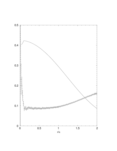
FIG. 1.: The bias function $\overline{H}(r)$ (top curve, solid line) used at $(\Gamma=40,\alpha^{*}=1)$ to determine the function $g_{w}(r)$ (bottom curve). The error bars on $g_{w}(r)$ correspond to two standard deviations.

FIG. 2.: Logarithm of the ratio $K(r)$ of the normalized $g_{0}(r)$ (standard MC calculation) and the unnormalized $g_{u}(r)$ (biased MC calculation) in the range $r_{min}<r<2a$ at $(\Gamma=40,\alpha^{*}=1)$.

FIG. 3.: The screening function $H(r)$ at $(\Gamma=40,\alpha^{*}=1)$ for a sample of $N=500$ particles. The standard MC calculation allows only the determination of $H(r)$ in the range $r_{min}<r<2a$ (curve on the right). The biased MC gives the curve in the range $r<2a$. In the overlapping region the agreement between these two estimates is satisfactory. The solid curve is a $6^{th}$ order even polynomial of the MC data

FIG. 4.: The screening function $H(r)$ for the OCP at $\Gamma=40$. Top curve: Ogata result. Bottom curves: MC data for a sample of $N=500$ ions (standard and biased simulations). The solid curve is a $6^{th}$ order even polynomial of the MC data.

FIG. 5.: The screening function $H(r)$ for the OCP. From bottom to top $\Gamma=1,2,10$, and $100$.

FIG. 6.: The screening function $H(r)$ for the YOCP at $\Gamma=40$ and some values of $\alpha^{*}$. From top to bottom $\alpha^{*}=0.,0.2,0.4,0.6,0.8,1.,1.2,1.4,2,$ and $3$.

REFERENCES

- [1] Hansen J P and Baus M 1980 Phys. Reports 59 1
- [2] Caillol J-M and Gilles D 2000 J. Stat. Phys. 100 905; ibid 100 933
- [3] Hamaguchi S and Farouki R T 1993 J. Chem. Phys. 101 9876; ibid. 9885
- [4] Ichimaru S 1993 Rev. Mod. Phys. 65 255
- [5] Torrie G and Patey G N 1977 Mol. Phys. 34 1623
- [6] Ogata S 1996 Phys. Rev. E 53 1094
- [7] Frenkel D and Smit B Understanding Molecular Simulations (Academic Press,1996)
- [8] Jancovici B 1977 J. Stat. Phys. 17 357
- [9] Rosenfeld Y 1996 J Stat. Phys. 53 2000
- [10] De Witt H and Slattery W 1999 Contrib. Plasma Phys. 39 97
- [11] Rosenfeld Y and Chabrier G 1997 J Stat. Phys. 89 283