Alexander’s prescription for colloidal charge renormalization

Abstract

The interactions between charged colloidal particles in an electrolyte may be described by usual Debye-Hückel theory provided the source of the electric field is suitably renormalized. For spherical colloids, we reconsider and simplify the treatment of the popular proposal put forward by Alexander et al. [J. Chem. Phys. 80, 5776 (1984)], which has proven efficient in predicting renormalized quantities (charge and salt content). We give explicit formulae for the effective charge and describe the most efficient way to apply Alexander’s et al. renormalization prescription in practice. Particular attention is paid to the definition of the relevant screening length, an issue that appears confuse in the literature.

I Introduction

The concept of charge renormalization is widely used in theories on effective interactions in charge-stabilized colloidal suspensions reviewBelloni97 ; levin:rev ; Likos ; Quesada . The basic idea is to consider the highly charged colloidal particle plus parts of the surrounding cloud of oppositely charged microions as an entity, carrying a renormalized charge $Z_{\mathrm{eff}}$ which may be orders of magnitude smaller than the actual bare charge $Z$ of the colloidal particle. Replacing $Z$ by $Z_{\mathrm{eff}}$, one can then use simple Debye-Hückel-like theories to calculate the effective interaction between two such colloidal particles in suspension. The pioneering work on colloidal charge renormalization is the paper by Alexander et al. alexander who proposed to calculate effective charges by finding, within the framework of the Poisson-Boltzmann cell model, the optimal linearized electrostatic potential matching the non-linear one at the cell boundary. In alexander , the prescription how to achieve this task, is given essentially in form of a numerical recipe which is often not the most convenient way possible. Making use of simple analytical expressions for effective charges recently suggested trizac1 ; trizac2 , we here describe an efficient way to realize Alexander’s et al. prescription for charge renormalization. In the infinite dilution limit of a colloid immersed in an infinite sea of electrolyte, explicit and accurate analytical expressions have been obtained only recently JPA , when the Debye length is smaller than the colloid size (spherical or cylindrical).

In order to illustrate the general significance of this celebrated charge renormalization concept, but also to demonstrate how broad its potential field of application is, we have selected a few recent studies which are – in one way or the other – concerned with Alexander’s et al. prescription. Experimentally, a variety of techniques can be used to determine effective charges of surfaces and spherical colloidal particles Behrens ; Wette ; vonGru3 , electrophoresis measurements Garbow ; Wette2 being certainly one of the most important. Other experiments, focusing on the colloid aggregation behavior Fernand ; Groenew , give direct evidence of the important role of counterion condensation and charge renormalization in colloidal systems. On the theoretical side, Yukawa-like interaction potentials with effective charges from Alexander’s et al. prescription are often used as the standard reference curves in calculations of effective interactions between charged colloids in suspensions Lobaski ; Terao2 ; Anta ; Mukherj ; Ulander , where, most recently, even discrete solvent effects Allahya ; Allahya2 ; Burak and density fluctuation effects Lukatsk are considered. Charge renormalization and nonlinear screening effects are also important when it comes to investigating the phase-behavior of charge-stabilized colloidal suspensions, be it the yet unsettled question of a possible gas-liquid phase-coexistence Diehl ; Schmitz1 ; vonGru ; deserno ; Tamashiro ; Tellez , or the solid-liquid phase-behavior Liu ; Schmitz . 3D charged colloidal crystals are rheo-optically investigated in Okubo , while defect dynamics and light-induced melting in 2D colloidal systems is in the focus of the studies in Pertsin and Beching2 ; Beching , respectively. Theories dealing with dynamic properties of charged colloidal suspensions are presented, for example, in Nagele1 . Another field of application are complexation problems: the complexation of a polyelectrolyte/DNA with spherical macroions Nguyen3 ; Nguyen , or, vice versa, the complexation of macroions with oppositely charged polyelectrolytes Nguyen2 ; Schiess ; Zhulina . Finally, we mention usage of Alexander’s et al. work in recent papers on microgels Levin , on the Rayleigh instability of charged droplets DDeserno , on charged spherical microemulsion and micellar systems Evilevi ; Piazza , and, as a last and more exotic example, in the theory of dusty plasmas Zagorod . We also note that the phenomenological concept of a Stern layer Stern –successfully applied in many studies on adsorption and micellization of ionic surfactants Kalinin – is reminiscent of the renormalization procedure under scrutiny here.

In section II, the general framework is presented, while Alexander’s et al. prescription is revisited in section III. Within such an approach, a natural screening parameter $\kappa_{\mathrm{PB}}$ appears, that plays the role of an inverse Debye length. In the literature, by analogy with the behavior of a bulk system, this parameter is often related to the mean (effective) micro-ion density $n^{*}$ in the suspension through the familiar expression $\kappa_{\mathrm{PB}}^{2}=8\pi\lambda_{B}n^{*}$, where $\lambda_{B}$ is the Bjerrum length. Such a relation follows from electroneutrality in the latter situation, but becomes incorrect in the confined geometry we shall be interested in. Particular emphasis will be put on this issue, when the colloidal suspension is dialyzed against a salt reservoir (section III.2), or put in the opposite limit of complete de-ionization (section III.3).

II Cell-model, Poisson-Boltzmann theory and Alexander’s et al. prescription

We consider a fluid of highly charged colloidal spheres having a radius $a$ and carrying each a total charge $-Ze$ ($e$ is the elementary charge). These colloids are suspended in a structureless medium of relative (CGS) dielectric constant $\varepsilon$ and temperature $T$ ($\beta=1/kT$), characterized by the Bjerrum length, $\lambda_{B}=\beta e^{2}/\varepsilon$ . The suspension is dialyzed against a reservoir of monovalent salt ions of a given pair concentration $c_{s}$ (the counterions are also assumed monovalent). Due to the fact that the colloid compartment is already occupied by the counterions originating from the macroions, the salt ion concentration in the reservoir, $c_{s}$, is always higher than the average salt ion density $n_{s}$ in the colloid compartment, an effect which is known as the Donnan-effect Dubois ; trizac40 ; deserno . Note that we not only have $n_{s}<c_{s}$ but also $n_{s}/(1-\eta)<c_{s}$, where $\eta$ is the volume fraction of the colloids [the mean density of salt ions in the volume accessible to microions is thus $n_{s}/(1-\eta)$ and not $n_{s}$]. By contrast, the total concentration of microions in the system (i.e. co-ions plus counter-ions) is larger than the total ion-concentration in the reservoir.

The work of Alexander et al. is based on the Poisson-Boltzmann cell model, an approximation which attempts to reduce the complicated many particle problem of interacting charged colloids and microions to an effective one-colloid-problem Marcus . It rests on the observation that at not too low volume fractions the colloids – due to mutual repulsion – arrange their positions such that each colloid has a region around it which is void from other colloids and which looks rather similar for different colloids. In other words, the Wigner-Seitz (WS) cells around two colloids are comparable in shape and volume. One now assumes that the total charge within each cell is exactly zero, that all cells have the same shape, and that one may approximate this shape such that it matches the symmetry of the colloid, i.e., spherical cells around spherical colloids. The cell radius $R$ is chosen such that $\eta=(a/R)^{3}$ equals the volume (or packing) fraction occupied by the colloids. If one neglects interactions between different cells, the thermodynamic potential of the whole suspension is equal to the number of cells times the thermodynamic potential of one cell. For a recent and more detailed description of the cell-model approximation see Ref. DeHo01 .

In a mean-field Poisson-Boltzmann (PB) approach, the key quantity to calculate is the local electrostatic mean-field potential $\phi({\mathbf{r}})$ (made dimensionless here by multiplication with $\beta e$), which thanks to the cell-model approximation has to be calculated in one WS cell only. It is generated by both the fixed colloidal charge density as well as the distributions $n_{\pm}({\mathbf{r}})=c_{s}e^{\mp\phi({\mathbf{r}})}$ of mobile monovalent ions, and follows from the PB equation, which together with the boundary conditions takes the form,

$$\begin{array}[]{rcl@{\hspace{1cm}}l}\nabla^{2}\phi(r)&=&\kappa_{\mathrm{res}}^{2}\sinh\phi(r)\hfil\hskip 28.45274pt&a<r<R\\ \vec{n}\cdot\nabla\phi(r)&=&Z\lambda_{B}/a^{2}\hfil\hskip 28.45274pt&r=a\\ \vec{n}\cdot\nabla\phi(r)&=&0\hfil\hskip 28.45274pt&r=R\end{array}$$ (1)

with $\vec{n}$ the outward pointing surface normal and the inverse screening length $\kappa_{\mathrm{res}}$ defined in terms of the ionic strength of the reservoir: $\kappa_{\mathrm{res}}^{2}=8\pi\lambda_{B}c_{s}$. Here we assume at $r=a$ the constant-charge boundary condition, and impose with the second boundary condition at $r=R$ the electroneutrality of the cell. As input parameter we have $Z$, $\kappa_{\mathrm{res}}$, $a$, $\lambda_{B}$ and $R$. But inspection of eq. (1) reveals that in fact only three parameters are really independent, which are $\kappa_{\mathrm{res}}a$ (reservoir salt concentration), $Z\lambda_{B}/a$ (colloidal charge) and $R/a$ (volume per colloid, i.e., volume fraction). Note that we have also tacitly assumed the electrostatic potential to vanish in the reservoir, where $n_{\pm}$ then becomes equal to $c_{s}$. The microionic charge density $\rho(r)$ can be written as

$$\rho(r)=n_{+}(r)-n_{-}(r)=-\frac{\kappa_{\mathrm{res}}^{2}}{4\pi\lambda_{B}}\sinh\phi(r)$$ (2)

and the microionic particle density as

$$\rho_{T}(r)=n_{+}(r)+n_{-}(r)=\frac{\kappa_{\mathrm{res}}^{2}}{4\pi\lambda_{B}}\cosh\phi(r)\>.$$ (3)

Hence,

$$Z=4\pi\int_{a}^{R}dr\>r^{2}\>\rho(r)$$ (4)

due to the electroneutrality of the cell, while the total number $2N_{s}+Z$ of microions in the cell is obtained from

$$2N_{s}+Z=4\pi\int_{a}^{R}dr\>r^{2}\>\rho_{T}(r)$$ (5)

where $N_{s}$ is the number of pairs of salt ions in the cell. We define the (”nominal”) salt concentration in the system as $n_{s}=N_{s}/V$ where $V=4\pi R^{3}/3$ is the volume of the WS cell. This volume should not be confused with that accessible to the microions $V_{\mathrm{free}}=4\pi(R^{3}-a^{3})/3=V(1-\eta)$. The ”net” salt ion concentration in the system then reads $n_{s}/(1-\eta)$, and due to the Donnan effect we have $n_{s}/(1-\eta)\leq c_{s}$.

Here is the point where we can describe Alexander’s et al. recipe for charge renormalization:

• solve the full non-linear problem, eq. (1), find the potential at $R$, $\phi_{R}$, and the total microion density, $n_{\pm}^{R}=c_{s}e^{\mp\phi_{R}}$,

• define the inverse screening constant from the microion density at WS boundary,

  $$\kappa_{\mathrm{PB}}^{2}=4\pi\lambda_{B}\Big{(}n_{+}^{R}+n_{-}^{R}\Big{)}=\kappa_{\mathrm{res}}^{2}\cosh\phi_{R}\>,$$ (6)

• linearize the boundary value problem in eq. (1) about $\phi=\phi_{R}$, determine the potential solution of the linearized PB equation such that linear and non-linear solution match up to the second derivative at $r=R$,

• compute the effective charge $Z_{\mathrm{eff}}$ from this solution by integrating the charge density associated with the linear solution from $a$ to $R$.

Replacing now ($Z$, $\kappa_{\mathrm{res}}$) by ($Z_{\mathrm{eff}}$, $\kappa_{\mathrm{PB}}$) in the effective Yukawa pair-potential of the DLVO (Derjaguin-Landau-Verwey-Overbeek) theory verwey ,

$$\beta v(r)=Z_{\mathrm{eff}}^{2}\lambda_{B}\left(\frac{e^{\kappa_{\mathrm{PB}}a}}{1+\kappa_{\mathrm{PB}}a}\right)^{2}\frac{e^{-\kappa_{\mathrm{PB}}r}}{r}\>,$$ (7)

one has succeeded in retaining an effective pair-interaction of the simple Yukawa form, even in cases where a high value of the bare charge $Z$ may violate the condition for the linearization approximation which this interaction potential is based on. While the relevance of defining an effective potential as (7) may be questioned at not too low density, the effective charge $Z_{\mathrm{eff}}$ and inverse screening length $\kappa_{\mathrm{PB}}$ are defined without ambiguity. It is also noteworthy that as an exact property of the cell model under study Lin , $\kappa_{\mathrm{PB}}$ is related to the pressure $P$ through

$$\beta P=\frac{1}{4\pi\lambda_{B}}\,\kappa_{\mathrm{PB}}^{2}.$$ (8)

III Alexander and collaborators’ prescription revisited

In the original paper of Alexander et al alexander , the procedure just described was introduced as a numerical recipe, and it was not pointed out that most of this scheme can actually be performed analytically. We now describe the more direct way to calculate Alexander’s et al effective charge which needs as input nothing but $\phi_{R}$ from the solution of eq. (1).

Let us consider the linearized version of eq. (1). We linearize the PB equation about $\phi_{R}$ and find

$$\nabla^{2}\widetilde{\phi}(r)=\kappa_{\mathrm{res}}^{2}\left[\gamma_{0}+\widetilde{\phi}(r)\right]\cosh\phi_{R}$$ (9)

where $\widetilde{\phi}=\phi-\phi_{R}$ and $\gamma_{0}=\tanh\phi_{R}$. We observe that the inverse screening length in eq. (9) is given by $\kappa_{\mathrm{res}}^{2}\cosh\phi_{R}$ which is just $\kappa_{\mathrm{PB}}^{2}$ from eq. (6), and thus just the value required in the Alexander et al. prescription. This observation shows that Alexander’s prescription, in essence, amounts to a certain linearization approximation where the potential value about which to linearize, is just the potential at the cell boundary $\phi_{R}$. Linearizing eq. (2) and (3), the microionic charge and particle densities now take the form

$$\rho(r) = -\frac{\kappa_{\mathrm{PB}}^{2}}{4\pi\lambda_{B}}(\gamma_{0}+\widetilde{\phi}(r))$$ (10)

$$\rho_{T}(r) = \frac{\kappa_{\mathrm{PB}}^{2}}{4\pi\lambda_{B}}(1+\gamma_{0}\widetilde{\phi}(r))\>.$$ (11)

With eq. (6), $\gamma_{0}$ can be rewritten as follows

$$\gamma_{0}=\tanh\phi_{R}=\sqrt{1-\left(\frac{\kappa_{\mathrm{res}}}{\kappa_{\mathrm{PB}}}\right)^{4}}\>.$$ (12)

Demanding that $\widetilde{\phi}(r)$ as well as its derivative are zero at $r=R$, we make sure that the solutions of the linearized and fully non-linear PB equation agree at the cell edge as required in Alexander’s et al. scheme. Taken together the boundary value problem of the linearized problem now reads,

$$\begin{array}[]{rcl@{\hspace{1cm}}l}\nabla^{2}\widetilde{\phi}(r)&=&\kappa_{\mathrm{PB}}^{2}(\gamma_{0}+\widetilde{\phi}(r))\hfil\hskip 28.45274pt&a<r<R\\ \widetilde{\phi}(r)&=&0\hfil\hskip 28.45274pt&r=R\\ \vec{n}\cdot\nabla\widetilde{\phi}(r)&=&0\hfil\hskip 28.45274pt&r=R\end{array}$$ (13)

Note that eq. (1) is a two-point boundary value problem, while eq. (13) represents a one-point boundary value problem.

III.1 Effective colloidal charges

The solution of eq. (13) is given by

$$\widetilde{\phi}(r)=\gamma_{0}\Big{[}-1+f_{+}\frac{e^{\kappa_{\mathrm{PB}}r}}{r}+f_{-}\frac{e^{-\kappa_{\mathrm{PB}}r}}{r}\Big{]}$$ (14)

with

$$f_{\pm}=\frac{\kappa_{\mathrm{PB}}R\pm 1}{2\kappa_{\mathrm{PB}}}\exp(\mp\kappa_{\mathrm{PB}}R).$$ (15)

With eq. (14) we can now easily calculate the effective charge by following eq. (4) and integrating eq. (10) over the cell volume, resulting in the simple formula

$$Z_{\mathrm{eff}}=\frac{\gamma_{0}}{\kappa_{\mathrm{PB}}\lambda_{B}}\Big{\{}(\kappa_{\mathrm{PB}}^{2}aR-1)\sinh[\kappa_{\mathrm{PB}}(R-a)]+\kappa_{\mathrm{PB}}(R-a)\cosh[\kappa_{\mathrm{PB}}(R-a)]\Big{\}}\>.$$ (16)

By comparison with the numerically calculated effective charges from Alexander’s et al. original prescription, we have explicitly checked that this formula indeed produces Alexander’s effective charges. Note that eq. (16) also follows from Gauss’ theorem applied at the surface of the colloid.

In summary, this then is the simple procedure to calculate renormalized charges:

• solve eq. (1) to obtain $\phi_{R}$,

• calculate $\kappa_{\mathrm{PB}}^{2}=\kappa_{\mathrm{res}}^{2}\cosh\phi_{R}$,

• insert this into eq. (16) to obtain $Z_{\mathrm{eff}}$.

We emphasize that once eq. (1) has been solved numerically, no further numerical fitting procedure is required to match the electrostatic potential from the linear and the non-linear solutions at $r=R$! In addition, the numerical solution of eq. (1) is much simplified by taking account of the technical points described in appendix A (see also appendix B for the salt free case).

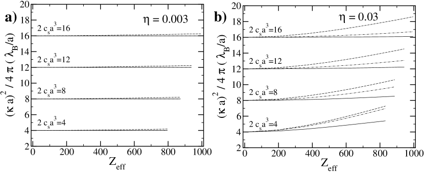
Figure 1: The inverse screening length $\kappa$ as a function of Alexander’s et al. effective charge $Z_{\mathrm{eff}}$ [eq. (16)] for various reservoir salt concentrations $c_{s}$ and two different colloid volume fractions [$\eta=0.003$ in a), and $\eta=0.03$ in b)]. Solid line: $\kappa_{\mathrm{PB}}^{2}$ from eq. (6), dashed line: $\kappa^{2}$ from eq. (21), dashed-dotted line: $\kappa_{\mathrm{PB}}^{2}|_{\gamma_{0}\to 0}$ from eq. (19). All curves terminate when the effective charge has reached its saturation value.

III.2 Effective salt concentration

Alexander’s original paper contains also a prescription how to calculate the effective salt concentration $n_{s}^{\mathrm{eff}}$. Again, we here can derive a simple formula. Integrating the particle density in eq. (11) over the cell volume accessible to the microions, as in eq. (5), we obtain

$$2N_{s}^{\mathrm{eff}}+Z_{\mathrm{eff}}=\frac{\kappa_{\mathrm{PB}}^{2}}{4\pi\lambda_{B}}V_{\mathrm{free}}(1-\gamma_{0}^{2})+Z_{\mathrm{eff}}\gamma_{0}$$ (17)

with $Z_{\mathrm{eff}}$ from eq. (16), so that

$$2n_{s}^{\mathrm{eff}}=\frac{\kappa_{\mathrm{PB}}^{2}}{4\pi\lambda_{B}}(1-\gamma_{0}^{2})(1-\eta)-Z_{\mathrm{eff}}n_{c}(1-\gamma_{0})\>,$$ (18)

where $n_{c}=1/V$ is the colloid density in the suspension and $n_{s}^{\mathrm{eff}}=N_{s}^{\mathrm{eff}}/V$. This formula is again successfully checked against the numerical values in Alexander’s et al. work. If $\gamma_{0}\to 0$, eq. (18) can be rearranged to give

$$\kappa_{\mathrm{PB}}^{2}\Big{|}_{\gamma_{0}\to 0}=\frac{1}{1-\eta}\,4\pi\lambda_{B}(Z_{\mathrm{eff}}n_{c}+2n_{s}^{\mathrm{eff}})\>.$$ (19)

Many studies, applying Alexander’s et al. renormalization concept, can be found in literature where $\kappa_{\mathrm{PB}}$ is computed not from eq. (6), as it should, but from

$$\kappa^{2}=\frac{1}{1-\eta}\,4\pi\lambda_{B}(Z_{\mathrm{eff}}n_{c}+2n_{s})\>,$$ (20)

or

$$\kappa^{2}=\,4\pi\lambda_{B}(Z_{\mathrm{eff}}n_{c}+2n_{s})\>,$$ (21)

with $Z_{\mathrm{eff}}$ from Alexander’s prescription and with $n_{s}$ being the actual (as opposed to ”effective”) salt concentration in the system. We here learn that this is certainly not the same as the $\kappa_{\mathrm{PB}}$ from eq. (6)! Indeed, Eqs. (20) and (21) rely on two further assumptions, namely that $\gamma_{0}$ can be set to zero and that $n_{s}\approx n_{s}^{\mathrm{eff}}$. Fig. (1) checks how good these approximations are. We restrict the following discussion to low values of the volume fraction $\eta$ so that expressions (20) and (21) coincide (the rather formal case of larger $\eta$ will be addressed in section III.3). For two volume fractions and various reservoir salt concentrations, we calculated in Fig. (1) the screening factor as a function of Alexander’s et al. effective charge obtained from eq. (16), (i) using eq. (6) (solid line), (ii) using the formula $4\pi\lambda_{B}(Z_{\mathrm{eff}}n_{c}+2n_{s}^{\mathrm{eff}})$ from eq. (19) with $n_{s}^{\mathrm{eff}}$ from eq. (18) (dashed-dotted line) and (iii) using $4\pi\lambda_{B}(Z_{\mathrm{eff}}n_{c}+2n_{s})$ from eq. (21) with $n_{s}$ from the non-linear calculation, i.e. from eq. (5) (dashed line). As $Z_{\mathrm{eff}}$ goes to zero, $n_{s}\to n_{s}^{\mathrm{eff}}$, $n_{s}\to c_{s}$ and $\phi_{R}\to 0$, so all three expressions must lead to the same $\kappa^{2}=8\pi\lambda_{B}c_{s}=\kappa_{\mathrm{res}}^{2}$. To be specific, we took typical values of aqueous colloidal systems for $a$ and $\lambda_{B}$ ($a=60$ nm, $\lambda_{B}=0.713$ nm). If however one wants to be a more general, one has to specify just $\kappa_{\mathrm{res}}a$, $Z\lambda_{B}/a$ and $\eta$ as these are the independent parameters of the problem. Multiplying the values of the x-axis with $\lambda_{B}/a$ and those of the y-axis with $4\pi\lambda_{B}/a$ where $\lambda_{B}/a=0.713/60=0.012$, one can transform Fig. (1) into a plot that is valid for systems characterized by other values of $a$ and $\lambda_{B}$. The two colloid volume fractions considered in Fig. (1) are both easily experimentally realizable. Note that the curves terminate at different $Z_{\mathrm{eff}}^{\mathrm{sat}}$ which is due to the fact that the saturation value of the effective charge depends on the salt content of the suspension trizac2 .

It is evident from the figure that for low volume fraction ($\eta=0.003$), it is of no consequence if the screening factor is calculated from eq. (6) or eq. (21), and the error is certainly negligible. At higher volume fraction, however, it is seen that both approximations involved in taking eq. (21) instead of eq. (6) – namely, $n_{s}\approx n_{s}^{\mathrm{eff}}$, and $\gamma_{0}\approx 0$ – take effect: both formulae, eq. (19) and (21), fail to give the correct value for $\kappa_{\mathrm{PB}}$ at low salt ($2c_{s}a^{3}=4$) and high $Z_{\mathrm{eff}}$, but the agreement between eq. (19) (dashed-dotted line) and $\kappa_{\mathrm{PB}}$ (solid line) improves if $c_{s}a^{3}$ increases, while eq. (21) still remains a rather poor approximation of $\kappa_{\mathrm{PB}}$. This means that at high salt concentration $\gamma_{0}\approx 0$ produces only a small error, while $n_{s}\approx n_{s}^{\mathrm{eff}}$ is always a bad approximation at high volume fraction, regardless the value of $c_{s}a^{3}$. We will refer to expression (21) as a ”naive” inverse screening length. While such an estimation is inappropriate in the context of Alexander and collaborators’ scheme, it is noteworthy that it naturally arises from a statistical mechanics treatment of electrostatic interactions in colloidal suspensions Chan1 ; Chan2 . This treatment is however performed within a linear theory formalism and therefore discards the non linear effects we are interested in the present article.

Often, $n_{s}$ is known from the experiment, while $c_{s}$ (and thus $\gamma_{0}$) is not, so that it seems to be difficult to calculate $n_{s}^{\mathrm{eff}}$ from eq. (18). However, it is not. One can obtain $n_{s}$ as a function of $c_{s}$, from the solution of eq. (1) by means of eq. (3) and (5). In cases where only $n_{s}$ is known from the experiment, one can then use this curve to find the $c_{s}$ corresponding to the known $n_{s}$. In fact, it is immaterial whether or not the experiment was actually performed with the system coupled to a particle reservoir. This becomes clear from the following consideration. Take a system coupled through a semi-permeable membrane to a salt reservoir with salt concentration $c_{s}$, and allow for some time till the Donnan equilibrium is reached. Then, the salt concentration in the system is $n_{s}/(1-\eta)\leq c_{s}$. Now, replace the semi-permeable wall by a unpenetrable wall and decouple the reservoir. The microion-distribution between the colloids and thus the screening factors will not change. In other words, in cases where the system is not coupled to a reservoir one can find a reservoir with an appropriately chosen $c_{s}$ which when coupled to the system would leave the microion density distribution in the system unaltered. This means that all our considerations presented are also valid for experiments in which the system is not coupled to a reservoir. This, of course, is strictly true only at a mean-field level of description. Practically, one then has to proceed as follows: (i) start from a trial value for $c_{s}$ and thus for $\kappa_{\mathrm{res}}^{2}=8\pi\lambda_{B}c_{s}$, (ii) solve eq. (1), (iii) calculate $n_{s}$ from eq. (3) and (5), (iv) vary $c_{s}$ and repeat (i) to (iii) until a $c_{s}=c_{s}^{exp}$ is found which leads to a $n_{s}$ that equals the $n^{exp}_{s}$ from the experiment. The pair $(n_{s}^{exp},c_{s}^{exp})$ can now be used in all the formulae presented above.

We close this section with a rather general remark. There is actually no need to linearize about the potential at the WS cell edge as done in eq. (13). An alternative is suggested by the following observation. Insert eq. (3) into eq. (5) and linearize about a potential $\bar{\phi}$,

$$2N_{s}+Z = \frac{\kappa_{\mathrm{res}}^{2}}{\lambda_{B}}\int_{a}^{R}dr\>r^{2}\>\cosh\phi(r)$$ (22)

$$\approx \frac{\kappa_{\mathrm{res}}^{2}}{\lambda_{B}}\int_{a}^{R}dr\>r^{2}\>\Big{[}\cosh\bar{\phi}+\sinh\bar{\phi}(\phi-\bar{\phi})\Big{]}\>.$$

If one now chooses

$$\bar{\phi}=\frac{4\pi}{V_{\mathrm{free}}}\int_{a}^{R}dr\>r^{2}\phi(r)\>,$$ (23)

then

$$2N_{s}^{\mathrm{eff}}+Z_{\mathrm{eff}}=\frac{\kappa_{\mathrm{res}}^{2}}{4\pi\lambda_{B}}V_{\mathrm{free}}\cosh\bar{\phi}$$ (24)

so that with $\kappa^{2}=\kappa_{\mathrm{res}}^{2}\cosh\bar{\phi}$ as in eq. (6) one obtains

$$\kappa^{2}=\frac{1}{1-\eta}\,4\pi\lambda_{B}(Z_{\mathrm{eff}}n_{c}+2n_{s}^{\mathrm{eff}})\>.$$ (25)

In words: linearizing not about the cell edge value of the potential, but about the average value of the potential in the cell (eq. (23)), leads to effective salt concentrations and effective charges which – when used to calculate the effective ionic strength – can be directly related to the inverse screening length in the way given by eq. (25), familiar from the Debye-Hückel theory. This linearization scheme is worked out in Trizacbis ; deserno ; Tamashiro , but does not correspond to the original proposal of Alexander et al.

III.3 Situation without added salt

In the limit where the system is in osmotic equilibrium with a reservoir of vanishing salt density ($c_{s}\to 0$), or in the canonical situation where no salt is added to the solution, the PB equation takes the form

$$\nabla^{2}\phi(r)=-\mu^{2}e^{-\phi(r)},$$ (26)

where $\mu$ is a prefactor whose value is determined through the electroneutrality constraint. We have

$$\kappa_{\mathrm{PB}}^{2}=4\pi\lambda_{B}n_{+}^{R}\,=\,\mu^{2}\,e^{-\phi_{R}}.$$ (27)

Equation (16), which provides the connection between the relevant screening parameter $\kappa_{\mathrm{PB}}$ and the effective charge $Z_{\mathrm{eff}}$, is still correct if $\gamma_{0}=1$ trizac2 . It is then tempting to compare $\kappa_{\mathrm{PB}}$ to the counterpart of expression (19):

$$\kappa^{2}=\frac{1}{1-\eta}\,4\pi\lambda_{B}Z_{\mathrm{eff}}n_{c}.$$ (28)

This comparison is shown in Fig. 2. Over a wide range of packing fractions, the ratio $\kappa/\kappa_{\mathrm{PB}}$ deviates from unity, but less than 30%. At relatively large bare charges, $Z$ and $Z_{\mathrm{eff}}$ differ significantly, so that neglect of charge renormalization in computing the screening parameter $\kappa$ [substitution of $Z_{\mathrm{eff}}$ by $Z$ in eq. (28)] badly fails compared to the “exact” $\kappa_{\mathrm{PB}}$.

Figure 2: Ratio of the “naive” inverse screening length $\kappa$ as given in eq. (28) over $\kappa_{\mathrm{PB}}$ defined from the microion density at the WS cell boundary, eq. (27), as a function of Alexander’s et al. rescaled effective charge $Z_{\mathrm{eff}}\lambda_{B}/a$ [eq. (16)], for various colloid packing fractions $\eta$ in the salt free case. The curves terminate at different $Z_{\mathrm{eff}}^{\mathrm{sat}}\lambda_{B}/a$ since the saturation value of the effective charge depends on the packing fraction Donnan .

It is instructive to investigate analytically a few limiting cases. We have computed $\kappa_{\mathrm{PB}}R$ from the solution of the non-linear PB. At fixed volume fraction, this quantity is bounded from above by its saturation value obtained when $Z\to\infty$. In the limit where the packing fraction $\eta$ vanishes, this saturation value $\kappa_{\mathrm{PB}}^{\mathrm{sat}}R$ is observed to vanish (although very slowly, as $-\eta^{1/3}\log\eta)$. Hence, $\kappa_{\mathrm{PB}}a=\eta^{1/3}\kappa_{\mathrm{PB}}R$ also vanishes, and this piece of information allows to linearize the exact relation (16), which then takes a simple form:

$$Z_{\mathrm{eff}}\frac{\lambda_{B}}{a}\,\sim\,\frac{1}{3}\,(\kappa_{\mathrm{PB}}R)^{2}\,\eta^{-1/3},$$ (29)

where the symbol $\sim$ stands for “asymptotically equivalent”. In other words, we have

$$\kappa_{\mathrm{PB}}^{2}\,\,\stackrel{{\scriptstyle\eta\to 0}}{{\sim}}\,\,4\pi\lambda_{B}Z_{\mathrm{eff}}n_{c},$$ (30)

so that $\kappa$ from eq. (28) and $\kappa_{\mathrm{PB}}$ coincide in this limit. It may be observed in Fig. 2 that $\eta=10^{-4}$ is not small enough to get the limiting behavior $\kappa/\kappa_{\mathrm{PB}}=1$, irrespective of $Z$ (and thus $Z_{\mathrm{eff}}$). In the opposite (and academic) limit where $\eta\to 1$, (i.e. $R\to a$), we obtain from (16)

$$\frac{\kappa}{\kappa_{\mathrm{PB}}}\,\,\stackrel{{\scriptstyle\eta\to 1}}{{\to}}\,\,1.$$ (31)

This last result somehow illustrates the relevance of the factor $1-\eta$ in (28). If the microions densities would have been defined with respect to the total volume of the cell and not the sub-volume accessible to microions, we would have obtained the alternative naive expression for the screening parameter

$$(\kappa^{\prime})^{2}=\,4\pi\lambda_{B}Z_{\mathrm{eff}}n_{c},$$ (32)

so that

$$\frac{\kappa^{\prime}}{\kappa_{\mathrm{PB}}}\,\,\stackrel{{\scriptstyle\eta\to 1}}{{\sim}}\,\,\sqrt{3(\eta^{2/3}-\eta)}\to 0.$$ (33)

Alternatively, in the limit of low bare charge $Z$ we get

$$Z_{\mathrm{eff}}\frac{\lambda_{B}}{a}\,\,\stackrel{{\scriptstyle Z\to 0}}{{\sim}}\,\,\frac{1}{3}\,\left(\frac{1}{\eta}-1\right)\,(\kappa_{\mathrm{PB}}\,a)^{2}.$$ (34)

As a consequence,

$$\frac{\kappa}{\kappa_{\mathrm{PB}}}\,\,\stackrel{{\scriptstyle Z\to 0}}{{\to}}\,\,1.$$ (35)

This feature may be observed in Fig 2 and is compatible with the result of eq. (30).

With added salt, similar argument may be put forward to provide an analytical relation between $\kappa_{\mathrm{PB}}/\kappa_{\mathrm{res}}$ and the density for e.g. large dilutions. Such expressions are nevertheless physically less transparent than those derived here for de-ionized suspensions, and have been omitted.

IV Conclusion

For colloidal spheres, we have reconsidered the original charge renormalization prescription proposed by Alexander et al. alexander . The computation of renormalized charge and salt content has been simplified in two respects: a) by the derivation of analytical expressions giving effective quantities as a function of parameters that are directly obtained from the solution of the non-linear PB problem; b) by converting the initial two-point boundary value non-linear PB problem into a computationally more convenient one-point boundary value problem (see appendices A and B). While we have restricted here to spherically symmetric polyions, similar considerations may be applied to the cylindrical geometry, relevant, e.g., to understand properties of solutions of charged polymers as for example the DNA molecule.

Once the effective charge and salt density are known, a “naive” screening parameter $\kappa$ may be defined as $\kappa^{2}=4\pi\lambda_{B}(Z_{\mathrm{eff}}n_{c}+2n_{s}^{\mathrm{eff}})/(1-\eta)$, where the factor $1-\eta$ accounts for the fact that a fraction $\eta$ of the Wigner-Seitz cell is not accessible to the microions. Strictly speaking, this inverse Debye length does not coincide in general with the relevant screening parameter $\kappa_{\mathrm{PB}}$, which has to be defined from the microions density at the WS boundary. In all the cases investigated here, the difference between $\kappa$ and $\kappa_{\mathrm{PB}}$ was less than 40%. Moreover, in the salt free case, $\kappa$ and $\kappa_{\mathrm{PB}}$ have been shown analytically to coincide for both low and large packing fractions (irrespective of the charge), and also for vanishing bare charges. This implies that the “naive”expression $\beta P=(Z_{\mathrm{eff}}n_{c}+2n_{s}^{\mathrm{eff}})/(1-\eta)$ yields a reasonable zeroth order equation of state for the suspension. On the other hand, neglect of charge renormalization, which amounts to defining $\kappa$ or $\beta P$ through the bare charge and salt density, appears to provide an extremely poor approximation for both $\kappa_{\mathrm{PB}}$ and the pressure.

Acknowledgments: We would like to thank Yan Levin and Jure Dobnikar for interesting discussions, and Mario Tamashiro for a careful reading of the manuscript.

Appendix A Numerical procedure with added electrolyte

In this appendix, we propose a few Mathematica${}^{\hbox{\scriptsize\textregistered}}$ lines of code to solve PB equation for a charged sphere in a concentric spherical Wigner-Seitz cell. To this end, all distances are rescaled with the diameter $a$ of the colloid, and the charge expressed in units of $a/\lambda_{B}$. It is convenient to recast the initial two point boundary value problem (1) into a one point boundary value problem by assigning an a priori value $\phi_{test}$ to the rescaled potential at WS boundary $\phi_{R}$. For the situation where $\kappa_{\mathrm{res}}a=2.0$ at a volume fraction $\eta=0.1$, the following procedure finds the corresponding solution (with the arbitrary choice $\phi_{test}=0.1$):

$$\kappa_{\mathrm{res}}=2.0\ ;\quad\eta=0.1\ ;\quad R=\eta^{-1/3}\ ;\quad\phi_{test}=0.1\ ;\quad sol=$$ (36)

$${\tt NDSolve}[\,\{\,2\phi^{\prime}[r]+r\phi^{\prime\prime}[r]==\kappa_{\mathrm{res}}^{2}r\,{\tt Sinh}[\phi[r]],\phi[R]==\phi_{test},\phi^{\prime}[R]==0\,\},$$

$$\qquad\qquad\qquad\phi,\{r,1,R\},{\tt WorkingPrecision}\to 20\,];\qquad\qquad$$

The potential $\phi$ may then be visualized as a function of $r/a$ with the command

$${\tt Plot}[\,{\tt Evaluate}[\phi[r]/.sol],\{r,1,R\}\,]$$ (37)

and the bare charge corresponding to the specific choice made for $\phi_{test}$ is obtained as the result of

$$(\,{\tt Evaluate}[\,\phi^{\prime}[1]/.sol\,]\,)\,[[1]].$$ (38)

With the above parameters, we get 2.55, which corresponds to the value of $Z\lambda_{B}/a$.

The limit $\phi_{test}\to 0$ corresponds to the limit $Z\to 0$. However, the solution of our one point boundary value problem only exists for $\phi_{test}\leq\phi_{sat}$, and the limit $\phi_{test}\to\phi_{sat}$ corresponds to $Z\to\infty$ which is equivalent to $Z_{\mathrm{eff}}\to Z_{\mathrm{eff}}^{\mathrm{sat}}$. Consequently, starting from low values of $\phi_{test}$, the solution associated with a targeted $Z$ is easily found by dichotomy, adjusting iteratively the values of $\phi_{test}$. For any value of $\phi_{test}$, $\kappa_{\mathrm{PB}}$ follows from eq. (6) and $Z_{\mathrm{eff}}$ is computed invoking eq. (16). For the parameters used in the example (36), the relation between $Z$, $Z_{\mathrm{eff}}$ and $\phi_{test}$ is illustrated in Figure 3.

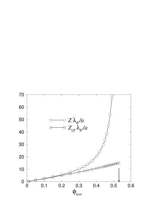
Figure 3: Bare and effective charges as a function of the “guess” boundary potential $\phi_{test}$. Here, $\kappa_{\mathrm{res}}a=2.0$ and the volume fraction is $10\%$. The arrow indicates the saturation value for $\phi_{test}$.

Appendix B Numerical procedure without added electrolyte

In the salt-free case, it is also convenient to rephrase the problem under study as a one point boundary value problem. At fixed bare charge, a possibility would be to consider the limit $\kappa_{\mathrm{res}}\to 0$ of a system in contact with a salt reservoir. In this (formally correct) limit, the corresponding $\phi_{test}$ diverges, and it turns out to be more convenient to impose that $\phi(R)=0$. This choice is such that $\mu=\kappa_{\mathrm{PB}}$ with the notations of eq. (27). Poisson’s equation (26) is then solved once a trial value has been chosen for $\mu$. For instance, with $\eta=0.1$ and $\mu=1.1$, the Mathematica${}^{\hbox{\scriptsize\textregistered}}$ line

$$\mu=1.1\ ;\quad\eta=0.1\ ;\quad R=\eta^{-1/3}\ ;$$ (39)

$$sol={\tt NDSolve}[\,\{2u^{\prime}[r]+ru^{\prime\prime}[r]==\mu^{2}r\,{\tt Exp}[u[r]],u[R]==0,u^{\prime}[R]==0\},$$

$$u,\{r,1,R\},{\tt WorkingPrecision}\to 20\,];\,\,\phi[r\!\_]:=({\tt Evaluate}[u[r]/.sol])[[1]];$$

allows to find the reduced potential $\phi$. The associated bare charge $Z\lambda_{B}/a$ is computed a posteriori from Gauss’ theorem

$$-({\tt Evaluate}[\phi^{\prime}[1]])$$ (40)

With the example described in eq. (39), we get 5.217. Here, $\mu$ plays a similar role in the resolution as $\phi_{test}$ in appendix A. The solution of eq. (26) only exists for $\mu<\mu^{\mathrm{sat}}$, and when $\mu\to\mu^{\mathrm{sat}}$ (i.e. when $\kappa_{\mathrm{PB}}\to\kappa_{\mathrm{PB}}^{\mathrm{sat}}$), the bare charge diverges. Implementing a PB-like cell problem along the lines described here constitutes a substantial simplification with respect to the traditional route, usually involving a Fortran or C code with a numerical fitting procedure of the linear and non-linear solutions of PB theory.

References

- (1) L. Belloni, Colloids Surfaces A 140, 227 (1998).
- (2) Y. Levin, Rep. Prog. Phys. 65, 1577 (2002).
- (3) C.N. Likos, Phys. Rep.-Rev. Sec. Phys. Lett. 348, 267 (2001).
- (4) M. Quesada-Perez, J. Callejas-Fernandez, and R. Hidalgo-Alvarez, Adv. Colloid Interface Sci. 95, 295 (2002).
- (5) S. Alexander, P.M. Chaikin, P. Grant, G.J. Morales, P. Pincus, and D. Hone, J. Chem. Phys. 80, 5776 (1984).
- (6) E. Trizac, L. Bocquet and M. Aubouy, Phys. Rev. Lett. 89, 248301 (2002).
- (7) L. Bocquet, E. Trizac and M. Aubouy, J. Chem. Phys. 117, 8138 (2002).
- (8) M. Aubouy, E. Trizac, L. Bocquet, to appear in J. Phys. A. (2003).
- (9) S.H. Behrens and D.G. Grier, J. Chem. Phys. 115, 6716 (2001).
- (10) P. Wette, H.J. Schöpe, and T. Palberg, J. Chem. Phys. 116, 10981 (2002).
- (11) H.H. von Grünberg, L. Helden, P. Leiderer, and C. Bechinger, J. Chem. Phys. 114, 10094 (2001).
- (12) N. Garbow, M. Evers, and T. Palberg, Colloid Surf. A-Physicochem. Eng. Asp. 195, 227 (2001).
- (13) P. Wette, H.J. Schöpe, R. Biehl, and T. Palberg, J. Chem. Phys. 114, 7556 (2001).
- (14) A. Fernandez-Nieves, A. Fernandez-Barbero, and F.J. de las Nieves, Phys. Rev. E 64, 032401 (2001).
- (15) J. Groenewold and W.K. Kegel, J. Phys. Chem. B 105, 11702 (2001).
- (16) V. Lobaskin, A. Lyubartsev, and P. Linse, Phys. Rev. E 63, 020401 (2001).
- (17) T. Terao and T. Nakayama, Colloid Surf. A-Physicochem. Eng. Asp. 182, 299 (2001).
- (18) J.A. Anta and S. Lago, J. Chem. Phys. 116, 10514 (2002).
- (19) A.K. Mukherjee, K.S. Schmitz, and L.B. Bhuiyan, Langmuir 18, 4210 (2002).
- (20) J. Ulander, H. Greberg, and R. Kjellander, J. Chem. Phys. 115, 7144 (2001).
- (21) E. Allahyarov and H. Löwen, J. Phys.: Condens. Matter 13, L277 (2001).
- (22) E. Allahyarov and H. Löwen, Phys. Rev. E 63, 041403 (2001).
- (23) Y. Burak and D. Andelman, J. Chem. Phys. 114, 3271 (2001).
- (24) D.B. Lukatsky and S.A. Safran, Phys. Rev. E 63, 011405 (2001).
- (25) A. Diehl, M.C. Barbosa, and Y. Levin, Europhys. Lett. 53, 86 (2001).
- (26) K.S. Schmitz, Phys. Rev. E 65, 061402 (2002).
- (27) H.H. von Grünberg, R. van Roij, and G. Klein, Europhys. Lett. 55, 580 (2001).
- (28) M.N. Tamashiro and H. Schiessel, e-print cond-mat/0210245.
- (29) G. Téllez and E. Trizac, J. Chem. Phys. at press, e-print cond-mat/0209114.
- (30) M. Deserno and H.H. von Grünberg, Phys. Rev. E 66, 011401 (2002).
- (31) K.S. Schmitz, Macroions in Solution and Colloidal Suspension (VCH, New York, 1993).
- (32) J.N. Liu, H.J. Schöpe, and T. Palberg, J. Chem. Phys. 116, 5901 (2002).
- (33) T. Okubo, H. Kimura, T. Hatta, and T. Kawai, Phys. Chem. Chem. Phys. 4, 2260 (2002).
- (34) A. Pertsinidis and X.S. Ling, Phys. Rev. Lett. 8709, 098303 (2001).
- (35) C. Bechinger, M. Brunner, and P. Leiderer, Phys. Rev. Lett. 86, 930 (2001).
- (36) C. Bechinger and E. Frey, J. Phys.: Condens. Matter 13, R321 (2001).
- (37) G. Nägele, M. Kollmann, R. Pesche, and A.J. Banchio, Mol. Phys. 100, 2921 (2002).
- (38) T.T. Nguyen and B.I. Shklovskii, J. Chem. Phys. 114, 5905 (2001).
- (39) T.T. Nguyen and B.I. Shklovskii, J. Chem. Phys. 115, 7298 (2001).
- (40) T.T. Nguyen and B.I. Shklovskii, Physica A 293, 324 (2001).
- (41) H. Schiessel, R.F. Bruinsma, and W.M. Gelbart, J. Chem. Phys. 115, 7245 (2001).
- (42) E. Zhulina, A.V. Dobrynin, and M. Rubinstein, Eur. Phys. J. E 5, 41 (2001).
- (43) Y. Levin, A. Diehl, A. Fernandez-Nieves, and A. Fernandez-Barbero, Phys. Rev. E 65, 036143 (2002).
- (44) M. Deserno, Eur. Phys. J. E 6, 163 (2001).
- (45) A. Evilevitch, V. Lobaskin, U. Olsson, P. Linse, and P. Schurtenberger, Langmuir 17, 1043 (2001).
- (46) R. Piazza and A. Guarino, Phys. Rev. Lett. 88, 208302 (2002).
- (47) A.G. Zagorodny, A.G. Sitenko, O.V. Bystrenko, P.P.J.M. Schram, and S.A. Trigger, Phys. Plasmas 8, 1893 (2001).
- (48) O. Stern, Ztschr. Elektrochem. 30, 508 (1924).
- (49) see e.g. V.V. Kalinin and C.J. Radke, Colloids Surf. A 114, 337 (1996); P.A. Kralchevsky, K.D. Danov, G. Broze and A. Mehreteab, Langmuir 15, 2351 (1999).
- (50) J.P. Hansen and E. Trizac, Physica A 235, 257 (1997).
- (51) M. Dubois, T. Zemb, L. Belloni, A. Delville, P. Levitz and R. Setton, J. Chem. Phys. 75, 944 (1992).
- (52) R.A. Marcus, J. Chem. Phys. 23, 1057 (1955).
- (53) M. Deserno and C. Holm, in: Proceedings of the NATO Advanced Study Institute on Electrostatic Effects in Soft Matter and Biophysics, ed. by C. Holm et al., Kluwer (2001).
- (54) E.J.W. Verwey and J.T.G. Overbeek, Theory of the Stability of Lyophobic Colloids (Elsevier, Amsterdam, 1948).
- (55) H. Wennerström, B. Jönsson and P. Linse, J. Chem. Phys. 76, 4665 (1982).
- (56) E. Trizac and J.-P. Hansen, Phys. Rev. E 56, 3137 (1997).
- (57) E. Trizac, M. Aubouy and L. Bocquet, to appear in J. Phys.: Condens. Matter 15, S291 (2003).
- (58) B. Beresford-Smith and D.Y.C. Chan, Chem. Phys. Lett. 92, 474 (1982).
- (59) B. Beresford-Smith and D.Y.C. Chan, J. Coll. Int. Sci. 105, 216 (1985).