Networks in life: Scaling properties and eigenvalue spectra

Abstract

We analyse growing networks ranging from collaboration graphs of scientists to the network of similarities defined among the various transcriptional profiles of living cells. For the explicit demonstration of the scale-free nature and hierarchical organization of these graphs, a deterministic construction is also used. We demonstrate the use of determining the eigenvalue spectra of sparse random graph models for the categorization of small measured networks.

PACS: 89.65.-s, 89.75.-k, 05.10.-a, 02.70.Hm

1 Introduction

Numerous natural, social and technological systems develop large complex structures made up from many similar, but still specific and individual units connected in a stochastic way. The simplest approach still rich in details to such phenomena uses random network models built upon ideas from random graph theory and statistical physics.

In this paper we give an overview of the major random graph models and also show an example for a determistic scale-free network. We analyse and model the social networks derived from scientific co-authorship data in mathematics and in neuroscience. For a more detailed description of random networks, we suggest the usage of spectral properties. Using a molecular biological network we demonstrate that the spectral characterization is appropriate for the categorization of measured networks even in the case of small systems made up of a few hundred nodes.

2 Network models

2.1 Stochastic graphs

The uncorrelated random graph model of Erdős and Rényi  [1] treats the network as an assembly of identical units, where the number of edges grows quadratically with the size of the system, $N$. However, in realistic cases, the number of edges grows less rapidly, e.g., linearly with system size. The small-world graph [2, 3] can be created by connecting each $1$st, $2$nd, …, $k$th neighbor pair of a one-dimensional periodic lattice and then randomly rewiring a given portion, $p_{\rm r}$, of the edges of the original regular graph. The resulting graph shows the small-world property: neighbors of an arbitrary vertex are often connected to each other, as well, but the number of steps (taken on the edges of the graph) connecting two arbitrary vertices tends to be low. In the stochastic scale-free model, one starts from $m$ isolated vertices, and at each time step one new vertex is added by connecting it to $m$ previous vertices. For a connection, any previous vertex is chosen with a probability proportional to its degree, $k_{i}$: $\Pi_{i}=k_{i}/\sum_{j=1,N}k_{j}$. In the infinite size limit, the distribution of degrees converges to a power-law, i.e., the system has no characteristic length scale.

2.2 Deterministic scale-free model

In the deterministic scale-free model [4] the network is built iteratively, each iteration repeating and reusing the already existing network. We start from a single node called the root of the network. Next, we add two nodes and connect each of them to the root of the network. In the nth time step we add two units identical to the already existing network (containing $3^{n-1}$ nodes each), and connect each of the $2^{n}$ bottom points (vertices) of these two units to the root point.

Due to the deterministic nature of the model, the degree distribution of hubs can be obtained exactly. In the limit, the asymptotic behavior of the degree distribution will depend only on the degrees of hubs, i.e., vertices having at least one further vertex below themselves. If we exclude the root point, the number of hubs with $k=2^{n-i+1}-2$ links after the $n$th iteration will be $N_{k}=(2/3)\,3^{i}$ ($i=1,...,n-1$). With the $N_{k}$ values known, a standard tool for obtaining the probability density, $p(k)$, of the graph’s degrees would be the cumulative density function, $\Phi(k)=N^{-1}\,\sum_{k}^{k_{max}}p(k^{\prime})$ ($N$ is the total number of hubs). However, for a clear illustration of the underlying mathematical idea, here we will give a slightly different derivation of the probability density of the graph’s degrees.

The above formulas of $k$ and $N_{k}$ will give $N_{k}\propto k^{-\log 3/\log 2}$ (which can be simplified to $N_{k/2}=3N_{k}$). When using this relation as a histogram of the probability density, the size of histogram bins (i.e., the separation between adjacent $k$ values) is proportional to $k$ itself. Thus, in the $N\to\infty$ limit we have

$$p(k)\propto k^{-1}\,N_{k}=k^{-(1+\log 3/\log 2)}\,.$$ (1)

for the degree distribution and $\gamma=1+\log 3/\log 2$ for the scaling exponent. For further recent proposals of deterministic scale-free models see Refs.  [5, 6].

3 Mathematics and neuroscience co-authorship networks

Social networks have been largely studied in social sciences  [7, 8]. A general feature of these studies is that they are restricted to rather small systems, and view networks as static graphs, whose nodes are individuals and links represent various social interactions. Recent statistical physics approaches focus instead on large networks, searching for universalities both in the topology of the web and in the dynamics governing it’s evolution. These combined theoretical and empirical results have opened unsuspected directions in many fields ranging from computer science to biology  [3, 7, 9, 10, 11, 12, 13, 14, 15].

To illustrate the power of these advances, here we summarize our results for the collaboration network of scientists. For each research field one can define a co-authorship network which reflects the professional links between the scientists. In this network nodes represent individual scientists, and two scientists are connected if they have ever published together. In order to gather information on the topology of a scientific co-authorship web, ideally, one would need a complete dataset of the published papers starting from the beginnings of the considered discipline until today. However, computer databases cover at most the past several decades. Thus any study of this kind needs to be limited to only a recent segment of the database, imposing unexpected challenges.

The databases considered by us contain article titles and authors of all relevant journals in the field of mathematics (M) and neuro-science (NS), published in the period 1991-98. In mathematics our database contains 70,975 different authors and 70,901 papers for an interval spanning eight years. In NS the number of different authors is 209,293 and the number of published papers is 210,750.

It is also important to mention that recently, Newman also applied modern network ideas to collaboration networks  [16, 17]. He studied large databases focussing on several fields of research over a five-year period, finding that collaboration networks possess all general ingredients of small-world networks  [16].

Figure 1: Degree distribution for the M and NS databases shown with logarithmic binning computed from the full dataset, cumulative up to 1998. The lines correspond to the best fits and have the slopes $2.1$ (NS, dotted) and $2.4$ (M, dashed).

3.1 Data analysis

In this section we analyse the topology and dynamics of the M and NS databases.

A quantity that has been much studied lately for various networks is the degree distribution, $P(k)$, giving the probability that a randomly selected node has $k$ links. The degree distributions of both the M and NS data indicate that collaboration networks are scale-free. The power-law tail is evident from the raw, uniformly binned data, but the scaling regime is better seen on the plot when logarithmic binning is applied to reduce the noise in the tail (Fig. 1).

Preferential attachment is part of all network models aiming to explain the emergence of the inhomogeneous network structure and power law connectivity distributions  [18, 19, 20]. For the networks considered by us preferential attachment appears at two levels:

(i) New nodes: For a new author preferential attachment means that it is more likely that his/her first paper will be co-authored with somebody who already has a large number of co-authors (links) than with another researcher having fewer collaborators. As a result ”old” authors with more links will increase their number of co-authors at a higher rate than those with fewer links. To investigate this process in quantitative terms we determined the probability that an old author with connectivity $k$ is selected by a new author for co-authorship. This probability defines the $\Pi(k)$ distribution function. Calling ”old authors” those present up to the last year, and ”new authors” those who were added during the last year, we computed the change in the number of links, $\Delta k$, for an old author with $k$ links at the beginning of the previous year, Plotting $\Delta k$ as a function of $k$ gives the function $\Pi(k)$, describing the nature of preferential attachment involved. Since measurements are limited to only a finite ($\Delta T=1$ year) interval, we improve the statistics by plotting the integral of $\Pi(k)$:

$$\kappa(k)=\int_{1}^{k}\Pi(k^{\prime})\,dk^{\prime}.$$ (2)

If preferential attachment is absent, $\Pi(k)$ should be independent of $k$, as each node grows independently of its degree, and $\kappa(k)$ is expected to be linear. As Fig. 2 shows, we find that $\kappa(k)$ is nonlinear, increasing as $\kappa(k)\sim k^{\nu+1}$, with the best fits giving $\nu\simeq 0.8$ for M and $\nu\simeq 0.75$ for NS.

(ii) Internal links: As the network evolves, a large number of new links appear between old nodes representing papers written by authors already part of the network, but having not collaborated before. These internal links are also subject to preferential attachment. We studied the probability $\Pi(k_{1},k_{2})$ that an old author with $k_{1}$ links forms a new link with another old author with $k_{2}$ links. The three dimensional plot of $\Pi(k_{1},k_{2})$ is shown in Fig. 3, the overall behavior indicating that $\Pi(k_{1},k_{2})$ increases as either $k_{1}$ or $k_{2}$ increases. Analysing in detail our data we also found that $\Pi(k_{1},k_{2})$ for internal links is approximately linear in $k_{1}k_{2}$.

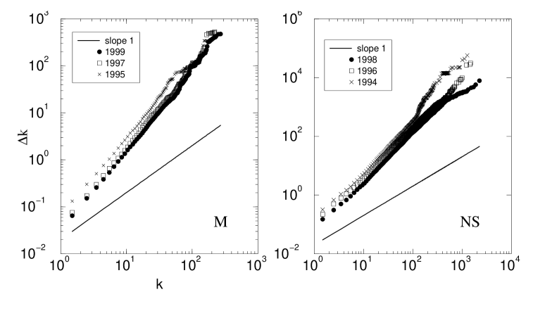
Figure 2: Cumulated preferential attachment ($\kappa(k)$) of incoming new nodes for the M and NS databases. In the absence of preferential attachment $\kappa(k)\sim k$, which shown as a continuous line on the figures.

Figure 3: Internal preferential attachment for the M and NS databases, 3D plots: $\Delta k$ as a function of $k_{1}$ and $k_{2}$. Results computed on the cumulative data in the last considered year.

4 Spectral characterization of random graphs

Suprisingly, not only human social networks, one of the highest levels of organization among living systems, but also food webs [21], molecular biological networks [14, 22] and the network of the similarities among various genetic programs of a single cell [23] display small-world and scale-free behavior.

However, until now, most analyses of the more realistic models and the analyses of data sets have been confined to the computation of quantities which are only loosely connected to structural properties: e.g., degree sequences, shortest connecting paths and clustering coefficients. Here, we will carry out a more detailed analysis using algebraic tools intrinsic to random graphs. Also, we will show that using algebraic tools suprisingly small measured networks, consisting of not more than a few hundred nodes, can be successfully classified into one of the realistic network model categories shown above.

4.1 Definitions and algorithms

Any graph $G$ can be represented by its adjacency matrix, $A(G)$, which is a real symmetric matrix: $A_{ij}=A_{ji}=1$, if vertices $i$ and $j$ are connected, or $0$, if these two vertices are not connected.

The spectrum of a graph is the set of eigenvalues of the graph’s adjacency matrix. The largest eigenvalue, $\lambda_{1}$, is also called the principal eigenvalue of the graph. To illustrate the meaning of the graph’s eigenvalues, consider the following example. Write each component of a vector $\vec{v}$ on the corresponding vertex of the graph: $v_{i}$ on vertex $i$. Next, on every vertex write the sum of the numbers found on the neighbors of vertex $i$. If the resulting vector is a multiple of $\vec{v}$, then $\vec{v}$ is an eigenvector, and the multiplier is the corresponding eigenvalue of the graph.

The spectral density, $\rho(\lambda)$, of a graph is the density of the eigenvalues of its adjacency matrix. For a finite system, this can be written as a sum of delta functions

$$\rho(\lambda):={1\over N}\sum_{j=1}^{N}\delta(\lambda-\lambda_{j})\,,$$ (3)

which converges to a continuous function with $N\to\infty$. The spectral density of a graph can be directly related to the graph’s topological features: the $k$th moment, $M_{k}$, of $\rho(\lambda)$ can be written as

$$M_{k}={1\over N}\sum_{j=1}^{N}(\lambda_{j})^{k}={1\over N}{\rm Tr}\big{(}A^{k}\big{)}=\ ={1\over N}\sum_{i_{1},i_{2},\cdots,i_{k}}A_{i_{1},i_{2}}A_{i_{2},i_{3}}\cdots A_{i_{k},i_{1}}\,.$$ (4)

From the topological point of view, $D_{k}=NM_{k}$ is the number of directed paths (loops) of the underlying – undirected – graph, that return to their starting vertex after $k$ steps (see Ref.  [24] for a detailed explanation).

4.2 Spectral densities of random graph models

In the infinite system size limit, the spectral density of an uncorrelated random graph – if rescaled as $\lambda^{\prime}=\lambda\,[Np(1-p)]^{-1/2}\propto\lambda\,N^{-1/2}$ – converges to a semi-circle:

$$\rho(\lambda^{\prime})=\ \cases{(2\pi)^{-1}\sqrt{4-\lambda^{\prime\,2}},&if \ $|\lambda^{\prime}|<2\sigma$;\cr 0,&otherwise.}$$ (5)

Suprisingly, the ideal semi-circular spectral density is not valid for any of the above mentioned realistic graph models [24, 25, 26]). In the sparse uncorrelated random graph the largest eigenvalue remains constant: $\lambda_{1}/pN\to c$, and $\rho(\lambda)$ will be symmetric in the infinite system size limit. Since the number of isolated clusters of any size will grow linearly with system size, the spectral density will contain an infinite number of singularities in the limit. Therefore, in the limit all odd moments ($M_{2k+1}$) converge to $0$. In other words: the number of all loops with odd length ($D_{2k+1}$) disappear. Since on a tree a path returning to its starting point must contain any edge an even number of times, the absence of loops with odd length indicates that the sparse uncorrelated random graph becomes more and more tree-like with $N\to\infty$. In other words, except for a few shortcuts a sparse uncorrelated random graph looks like a tree.

We conclude, that – from the spectrum’s point of view – the high number of triangles is one of the most basic properties of the small-world model, and it is preserved much longer, than regularity or periodicity, if the level of randomness, $p_{\rm r}$, is increased. Note that the high number of triangles is equivalent to a high average clustering, $C$, of the graph.

Figure 4: Main panel: The average spectral densities of scale-free graphs with $m=m_{0}=5$, and $N=100$ (—), $N=1000$ (– –) and $N=7000$ (- - -) vertices. (For $N=100$ and $N=1000$, the complete spectrum of $1000$ graphs, and for $N=7000$, the complete spectrum of $25$ graphs was used.) Another continuous line shows the semi-circular distribution for comparison. Observe that (i) the central part of the scale-free graph’s spectral density is triangle-like, not semi-circular and (ii) the edges show a power-law decay, whereas the the semi-circular distribution’s edges decay exponentially [28]. Inset: The upper and lower tails of $\rho(\lambda)$ (open and full triangles) for scale-free graphs with $N=40,000$ vertices the average degree of a vertex being $\langle k_{i}\rangle=2m=10$, as before. Note that both axes are logarithmic and $\rho(\lambda)$ has a power-law tail with the same decay rate at both ends of the spectrum. The line with the slope $-5$ in this figure is a guide to the eye.

For $m=m_{0}=1$, the scale-free graph is a tree by definition and its spectrum is symmetric [27]. In the $m>1$ case $\rho(\lambda)$ consists of several well distinguishable parts (see Fig. 4). The “bulk” part of the spectral density – the set of the eigenvalues {$\lambda_{2},...,\lambda_{N}$} – converges to a symmetric continuous function, which has a triangle-like shape for $|\lambda^{\prime}|<1.5$ and has power-law tails.

The central part of the spectral density converges to a triangle-like shape with its top lying well above the semi-circle. Since the scale-free graph is fully connected by definition, the increased number of eigenvalues with small magnitudes cannot be accounted to small isolated clusters. (All $N$ eigenvalues of a finite-sized isolated cluster with $N$ vertices fall between $-\sqrt{N}$ and $\sqrt{N}$.) As an explanation, we suggest, that the eigenvectors of these eigenvalues are localized on a small subset of the graph’s vertices.

The inset of Fig. 4 shows the tail of the bulk part of the spectral density for a graph with $N=20,000$ vertices and $100,000$ edges (i.e., $pN=10$).

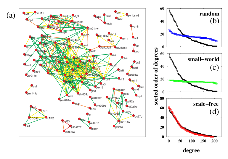
Figure 5: (a) The transcriptome similarity network of Ref. [23]. Each link is colored according to its predicted strength: dark links indicate strong coupling. (b-d) Analysis of the graph’s largest component (the data graph). On each analysis plot black $+$ signs show data points and open gray boxes show data points of the three random graph models. The data graph and all three test graphs have the same number of edges and vertices. The almost complete overlapping of data and test points on subfigure (d) indicates that the transcriptome similarity graph is scale-free.

4.3 Application: classification of a molecular biological network by spectral methods

Figure 5 shows a biochemical network derived from recent gene expression data (see Refs. [23, 29] for an explanation). Nodes of the graph represent individual genetic programs (also called transcriptomes) of a cell in response to various internal or external perturbations. A connection between two nodes indicates that according to the applied similarity search algorithm [23], which compares each pair of the genetic programs individually, the two indicated transcriptomes contain a high number of regions with strong correlation ($|C|>0.8$) of gene expression.

Besides the transcriptome similarity graph, Figure  5 also shows its spectral analysis by comparing the largest component to three idealized test graphs with the same number of edges and vertices. Note that on the inverse participation ratio vs. eigenvalue plots the best fit is given by the scale-free graph, which almost completely overlaps with the measured graph’s data. The principal eigenvalue and the inverse participation ratio of the first eigenvector are both high in the measured and the scale-free graphs, whereas they are both significantly lower in the two other models. This indicates that the largest component of the transcriptome similarity graph is scale-free and a handful of its vertices are structurally dominant.

References

- [1] P. Erdős and A. Rényi, “On the evolution of random graphs,” Publ. of the Math. Inst. of the Hung. Acad. of Sci. 5 (1960) 17-61
- [2] D. J. Watts, Small World (Princeton University Press, Princeton, 1999).
- [3] D. J. Watts and S. H. Strogatz, “Collective dynamics of ‘small-world’ networks,” Nature 393 (1998) 440-442
- [4] A.-L. Barabási, E. Ravasz and T. Vicsek, “Deterministic scale-free networks,” Physica A 299, 599-564 (2001)
- [5] S. N. Dorogovtsev, A. V. Goltsev and J. F. F. Mendes, (to be published).
- [6] S. Jung, S. Kim and B. Kahng, Phys. Rev. E 65 056101 (2002).
- [7] S. Wasserman and K. Faust, Social Network Analysis (Cambridge Univ. Press, Cambridge, 1994).
- [8] M. Kochen (ed.) The Small World (Ablex, Norwood, NJ, 1989).
- [9] L. A. N. Amaral, A. Scala, M. Barthélémy and H. E. Stanley, Proc. Nat. Acad. Sci. USA 97, 11149 (2000).
- [10] R. Albert and A. L. Barabási, Phys. Rev. Lett. 85, 5234 (2000).
- [11] R. Albert, H. Jeong and A.L. Barabási, Nature 400, 130 (1999).
- [12] S. Lawrence and C. L. Giles, Nature 400 107 (1999).
- [13] B. A. Huberman and L. A. Adamic, Nature 401 131 (1999);
- [14] H. Jeong et al., Nature 407, 651 (2000).
- [15] R. V. Solé and J. M. Montoya, cond-mat/0011196 (2000);
- [16] M. E. J. Newman, Proc. Nat. Acad. Sci. USA 98, 404 (2001).
- [17] M. E. J. Newman Phys.Rev. E 64 016131 (2001).
- [18] S. N. Dorogovtsev and J. F. F. Mendes, Europhys. Lett. 52, 33 (2000).
- [19] S. N. Dorogovtsev and J. F. F. Mendes, Phys. Rev. E 62, 1842 (2000).
- [20] P. L. Krapivsky, S. Redner and F. Leyvraz, Phys. Rev. Lett 85, 4629 (2000);
- [21] J. M. Montoya and R. V. Solé, “Small World Patterns in Food Webs,” cond-mat/0011195
- [22] S. Wuchty, “Scale-Free Behavior in Protein Domain Networks,” Mol. Biol. Evol. 18 1694-1702 (2001)
- [23] I. J. Farkas, H. Jeong, T. Vicsek, A.-L. Barabási and Z. N. Oltvai (to be published)
- [24] I. J. Farkas, I. Derényi, A.-L. Barabási and T. Vicsek, Phys. Rev. E 64, 026704:1-12 (2001)
- [25] M. Bauer, O. Golinelli, “Random incidence matrices: moments of the spectral density,” J. Stat. Phys. 103, 301-337 (2001)
- [26] K.-I. Goh, B. Kahng and D. Kim, “Spectra and eigenvectors of scale-free networks,” Phys. Rev. E 64, 051903 (2001)
- [27] D. M. Cvetković, M. Doob and H. Sachs, Spectra of Graphs (Berlin, 1980)
- [28] M. L. Mehta. Random Matrices. 2nd ed. (Academic, New York, 1991)
- [29] T. R. Hughes, et.al., “Functional discovery via a compendium of expression profiles,” Cell 102, 109-126 (2000)