Abstract

Molecular dynamics (MD) simulations of crystalline poly(ethylene oxide) (PEO) have been carried out in order to study its vibrational properties. The vibrational density of states has been calculated using a normal mode analysis (NMA) and also through the velocity autocorrelation function of the atoms. Results agree well with experimental spectroscopic data. System size effects in the crystalline state, studied through a comparison between results for 16 unit cells and that for one unit cell has shown important differences in the features below 100 cm^-1. Effects of interchain interactions are examined by a comparison of the spectra in the condensed state to that obtained for an isolated oligomer of ethylene oxide. Calculations of the local character of the modes indicate the presence of collective excitations for frequencies lower than 100 cm^-1, in which around 8 to 12 successive atoms of the polymer backbone participate. The backbone twisting of helical chains about their long axes is dominant in these low frequency modes.

1 Introduction

Solid polymer electrolytes (SPE), composed of inorganic salts solvated in solid, high molecular weight polymer matrices, have been the focus of intense theoretical and experimental research because of their applications as solid state batteries [1, 2]. In spite of their wide technological applications, the precise mechanism of conduction in these materials is still unclear and remains a pursuit of interest. In non-polymeric crystalline and glassy electrolytes, the ionic species hop from one site to another within a rigid host frame. However, the conduction mechanism in solid polymer electrolytes is believed to be different [3, 4, 5]. NMR studies of line shape and relaxation rates in poly(ethylene oxide)-lithium salt complexes have demonstrated a relationship between the motion of the Li⁺ ions and the segmental motion of the PEO chains [6]. This notion gains support from other experimental studies such as Field-Gradient NMR spin echo technique [7], and Quasi-elastic Neutron Scattering (QENS) [8]. SPE, in general, contain both amorphous and crystalline regions, with conduction being facile in the amorphous regions. This is probably due to differences in the chain dynamics [9]. The work of Armand and coworkers has shown that ion mobility in solid electrolytes is of a continuous, diffusive type, in the amorphous regions [10]. NMR, differential scanning calorimetry and electrical conductivity studies have demonstrated that both cations and anions are mobile in the amorphous phase [11]. Recently, Bruce and coworkers have shown that a SPE with a ratio of ether oxygen to lithium of 6:1, exhibits higher conductivity in its crystalline phase as compared to its amorphous phase and that the ion transport is dominated by the cations [12]. In such complexes, cross-linking between a pair of polymer chains results in a channel like structure. The ion moves in this channel, aided by the segmental motion of the polymer chain pair.

A large number of simulations have been carried out on PEO and PEO-salt complexes, both in their crystalline and amorphous phases over the last decade. Molecular dynamics studies by de Leeuw et al, using an united atom model (UAM) for PEO chains in their molten state, have examined the motion of methylene groups which they term as segmental motion [13]. Neyertz et al have performed extensive molecular dynamics simulations of bulk crystalline PEO [14, 15], PEO melts [16], crystalline NaI-PEO [17] and amorphous NaI-PEO [18] systems. The simulations of Muller-Plathe and coworkers on PEO-LiI complexes [19] have demonstrated that the ether oxygens belonging to consecutive monomers of a PEO chain coordinate to the same $Li^{+}$ ion and that this segmental coordination is argued to be the driving force for salt dissolution. Laasonen and Klein have performed MD simulations of both crystalline and amorphous PEO-NaI complexes [20]. Their study showed that ion pairing is most probable in the crystalline rather than in the amorphous phase. Halley and coworkers have studied the structure of amorphous PEO using the Parrinello-Rahman method recently [21]. MD simulations have also been employed by Smith and coworkers to elucidate the structure and dynamics of poly(propylene oxide) melts [22], PEO-salt complexes [23] and aqueous PEO solutions [24], using a potential model derived from ab initio calculations [25].

It is our endeavor here to characterize the vibrational modes of the polymer backbone in the pristine polymer, with an emphasis on the low frequency modes. This could enhance our understanding on the exact relationship between the dynamics of the polymer and that of the cation in the PEO-salt complexes. We carry out this study with the thought that understanding the evolution of the vibrational modes from the crystalline phase of pure PEO to its nature in the glassy state without and with the salt is crucial in mapping the precise mechanism of ion transport in these systems [26, 27]. Normal mode analyses to characterize vibrational spectra have been employed successfully to describe the dynamics of glassy systems [28], and are likely to be employed in the study of jammed granular materials [29]. These calculations have also helped our understanding of vibrational modes of polyethylene [30], of proteins in solution [31], and in determining the flexibility of proteins, and in the thermodynamics of hydration water in protein solutions [32]. Unlike polyethylene, PEO adopts a distorted helical conformation in its crystalline state, with the distortion arising from strong intermolecular interactions. It is thus important that such normal mode calculations be performed for the crystalline state, rather than for an isolated oligomer. In this paper, we limit ourselves to the study of the vibrational spectrum of PEO in its crystalline state. Analyses of these modes under other state and phase conditions will be examined in future. In anticipation of our results, we have identified the existence of segments in the polymer backbone consisting of around 8 to 12 atoms, to exhibit significant atomic displacements, for vibrational modes with frequencies up to around 100 cm^-1, and that the modes with frequencies below 60 cm^-1 involve twisting of the skeletal backbone. The paper is divided as follows. Details of the simulation and the methods of analyses are presented in the next section. Later, we discuss the results obtained from our study. Details on obtaining the elements of the dynamical matrix are provided in the Appendix.

2 Details of Simulation

The unit cell of crystalline PEO is monoclinic with the PEO chains in a (7/2) distorted helical conformation with TTG sequence [33]. An unitcell consists of four PEO chains with 21 backbone atoms in each chain. The MD runs reported here were initiated from configurations generated from this crystal structure. The two ends of a polymer chain were assumed to be bonded across the simulation cell boundary [14, 20] to eliminate end effects. MD simulations were performed primarily for a system that we describe as $\langle 422\rangle$, which contained 4 unitcells along the a-axis, 2 unitcells along the b-axis and 2 unitcells along the c-axis, containing a total of 3136 atoms. To study system size effects and effects of inter-chain interactions, we have performed additional simulations of only one unitcell, and also of one isolated finite length polymer chain. Thus the simulations for the $\langle 422\rangle$ cells and that for the one unitcell contained chains that had no ends, while that for the isolated molecule, contained a chain with two ends. An all atom model (AAM), with explicit consideration of hydrogen atoms was used, to properly account for the steric interactions expected to be dominant in the crystalline state. The simulations were carried out in the canonical ensemble at 5K for the NMA and in the constant pressure ensemble at 300K and 1 atmosphere to test the stability of the simulated crystal. Temperature control was achieved by the use of Nose-Hoover chain thermostats [34], using the PINY-MD program [35]. Long range interactions were treated using the Ewald method with an $\alpha$ value of 0.3 Å^-1, and 2399 reciprocal space points were included in the Ewald sum [36]. The methylene groups were treated as rigid entities, enabling us to employ a timestep of 1 fs. To obtain the vibrational density of states, we performed these calculations at a temperature of 5K, where the atoms could be expected to be near their equilibrium positions. The equilibration period for the single molecule, the unitcell, and the $\langle 422\rangle$ system were 65 ps, 100 ps, and 750 ps, respectively. These were followed by an analysis run of duration 30 ps during which the coordinates and velocities of each particle were stored at regular intervals. Velocities were dumped every time step to obtain the power spectrum of their time correlation functions and the coordinates were dumped every 10 fs.

The simulations were performed with a force field obtained from the work of Neyertz [14] with the torsional parameters of the CHARMm model [37]. The potential parameters are given in Table 1. The non-bonded interactions were truncated at 12Å for the $\langle 422\rangle$ crystal, at 3.25Å for one unitcell, and at 12Å for the single molecule runs. The lower cutoff value for the unitcell run is necessitated by the fact that the interaction cutoff should be less than half of the minimum distance between any two opposite faces of the simulation cell.

The potential energy of the system can be expanded in terms of atomic displacements from an equilibrium configuration as,

$$U\left(q_{1},q_{2},...,q_{n}\right)=U\left(q_{01},q_{02},...,q_{0n}\right)+\left(\frac{\partial U}{\partial q_{i}}\right)_{0}\eta_{i}+\frac{1}{2}\left(\frac{\partial^{2}U}{\partial q_{i}\partial q_{j}}\right)_{0}\eta_{i}\eta_{j}+...$$ (1)

where the subscript 0 represents the equilibrium configuration and $\eta_{i}$ are the deviations of the coordinates from equilibrium, represented as,

$$q_{i}=q_{0i}+\eta_{i}$$ (2)

The elements of the Hessian matrix are given by

$$H^{\alpha\beta}_{ij}=\frac{1}{\sqrt{m_{i}m_{j}}}\left(\frac{\partial^{2}U}{\partial\beta_{j}\partial\alpha_{i}}\right)$$ (3)

where i,j represent particle indices and $\alpha$, $\beta$ represent the spatial coordinates x,y,z. $m_{i}$ is the mass of particle i. A simple scheme to obtain some of these Hessian elements efficiently is provided in the Appendix. All Hessian elements obtained from such analytical expressions were checked against numerical second derivatives [38] within our normal mode analysis code, and were found to match. The eigenvalues and eigenvectors of the Hessian matrix were examined to understand the vibrational dynamics of PEO. The frequency, $\nu_{s}$ ,of a particular mode of vibration, s, is related to its eigen value, $\lambda_{s}$ , by

$$\lambda_{s}=\left(2\pi\nu_{s}\right)^{2}$$ (4)

With these set of interactions, the initial pressure of the $\langle 422\rangle$ system was found to be around 4000 atmospheres. Hence, we performed a MD run in the NPT ensemble for 200 ps under ambient conditions. The change in volume was found to be 1.3% from that of the experimental crystal. Time correlation functions of atomic velocities were calculated, and were Fourier transformed to obtain the power spectra. These were compared with the spectrum obtained from the NMA. The spectra were convoluted with a Gaussian function of width 4cm^-1 so as to provide a width to the spectral features. The helical axis of a PEO chain possesses a 7-fold rotational symmetry. In addition, 7 C₂ axes lie perpendicular to it, making the molecular symmetry of PEO to be D₇ [33]. We have characterized the symmetry of the normal modes by studying the transformation of atomic displacements, on application of the symmetry operations for this group. Specifically, the operation by the C₂ axes enables a distinction between the three irreducible representations, A₁, A₂, and E.

We have also characterized the spatial extent of the modes of vibration using a quantity called the local character, defined as [31, 39]

$$Localcharacter\left(j\right)=\sum_{i=1}^{3N}u_{ij}^{4}$$ (5)

where $u_{ij}$ is the i^th component of the j^th eigenvector. The local character value can range from 0 to 1 and it determines the extent of localization of a particular mode.

To obtain quantitative information on the length of the segment involved in the low frequency modes, we have defined a quantity called the Continuous Segment Size (CSS). We calculate the displacement of the $k^{th}$ atom due to a $i^{th}$ mode using the expression

$$<\delta r^{2}_{ik}>=k_{\rm B}T\frac{\bracevert\vec{u}_{i}^{k}\bracevert^{2}}{m_{k}\omega_{i}^{2}}$$ (6)

where $m_{k}$ is mass of $k^{th}$ atom, $\vec{u}_{i}^{k}$ is the vector formed by the components of the i^th eigen vector contributed by the k^th atom, $T$ is temperature, and $\omega_{i}$ is the frequency of the i^th normal mode. We then check if the displacement is greater than a specified cutoff. If $n$ successive backbone atoms of a chain each have displacements greater than the displacement cutoff, they are defined to constitute a segment with CSS = $n$. Similarly, CSS was calculated for all possible modes with different vibrational frequencies from which the average segment size for a given frequency was calculated.

3 Results and Discussion

For crystalline systems, a close match between the experimentally determined cell parameters and that obtained from simulations is a crucial first step in the veracity of the parameters used. We show in Figure 1, the time evolution of the cell parameters at 300K and 1 atmospheres, generated by a MD run in the constant pressure ensemble using the Parrinello-Rahman method [40]. The $b$ and the $\beta$ parameters of the unit cell exhibit a relaxation from the zero time experimental value, due possibly to relatively minor deficiencies in the interaction model used to represent this system. The constancy of the cell parameters for over 100 ps, shows that the simulated crystal is in a stable state, and that the potential parameters are indeed able to reproduce the high demands of the crystal symmetry. Table 2 compares the cell parameters obtained from our simulations to the experimental data.

An interesting feature associated with polymer dynamics is the variation of the various vibrational modes of a chain encountered during its transformation from the isolated state to the crystalline state. The vibrational spectra of a single molecule, one unitcell and that of the $\langle 422\rangle$ crystal are compared in Figure 2a. When the chains assemble to form a crystal, each chain might prefer a new conformational state relative to its structure in the isolated state. A comparison of the vibrational spectra between that of one isolated molecule of finite length and of the $\langle 422\rangle$ system provides information on the effect of intermolecular interactions. As expected, the vibrational states of the isolated molecule showed marked differences from the crystalline state, particularly in the low frequency regions, where large amplitude, collective motions are predominant (see later). However, there are no significant changes in the high frequency regions of the spectrum. The spectrum for the one unitcell compares well with that of the $\langle 422\rangle$ crystal. However, the features in the VDOS of the $\langle 422\rangle$ crystal is much better resolved, particularly at low frequencies. For instance, the features at around 40 cm^-1 and 75 cm^-1 are clearly evident in the larger system than in the spectrum for the unitcell, pointing to effects of long range interactions. The spectrum for the $\langle 422\rangle$ system is shown in an expanded scale in Figure 2b. The split in the feature below 100 cm^-1 is evident and compares well with experimental infrared (IR) spectra [41] that shows features at 37 cm^-1, 52 cm^-1, 81 cm^-1 and 107 cm^-1. We do observe a prominent shoulder at 108 cm^-1 which has been attributed to modes involving C-O internal rotation earlier [41]. A comparison of the simulated vibrational density of states with the experimental IR and Raman spectra, exhibited in Figure 2c, shows that the potential model captures well nearly all the vibrational modes [41, 42, 43]. Note that the simulated spectrum is the raw density of states and does not contain any other terms that are needed to calculate the experimental spectra. Thus only the peak positions need to be compared, and not their intensities. Almost all the features found in the IR and Raman spectra seem to be present in the simulated VDOS. Another noteworthy feature of the spectrum is the absence of modes with imaginary frequencies which would have corresponded to either the presence of atoms away from equilibrium locations or to a mismatch between the empirical potential function and the crystal structure.

We have also calculated the vibrational spectrum through the Fourier transformation of the velocity auto correlation function of the atoms. This is compared with the VDOS obtained by the NMA in Figure 3. The agreement between the spectra is excellent except for features above 1200 cm^-1. Also, the peak at around 1470 cm^-1 is missing in the spectrum obtained through the velocity autocorrelation function (VACF). Visualization of the atomic displacements associated with this mode revealed HCH bending in methylene groups. Since all the CH₂ groups were constrained to be rigid during the MD runs for the VACF analysis, the absence of a peak in the VDOS obtained from VACF, in this region can be rationalized. The comparison of the VDOS obtained from the two methods is good, despite the fact that the NMA method is only a harmonic approximation to the potential. Close examination of the two shows a marginal (approximately 4-5 cm^-1) shift to higher frequencies in the spectrum obtained by the NMA method relative to that from the VACF.

We visualized the eigenvectors corresponding to different vibrational modes to assign the nature of atomic displacements that are responsible for the spectral features. In general, our assignments are consistent with earlier calculations [44, 45]. In Figure 4a and Figure 4b, we display a few of the modes. The zero frequency mode characterizes rigid body translation. The features at around 40 cm^-1, have earlier been attributed to chain deformations [41]. Based on visualization of atomic displacements shown in Figure 4a, we assign these modes specifically to the twisting of the polymer backbone. The mode at 88 cm^-1 arises from torsional motion around the C-O bond. The A₁ mode at 216 cm^-1 can be assigned to torsions around the C-C bond, while the 510 cm^-1 feature involves bending of CCO triplets. COC bending is observed at 952 cm^-1 while the wagging motion of the methylene groups is found to be present at 1244 cm^-1, in good agreement with IR and Raman measurements [44]. The symmetry of the modes are also shown in Figures 4 agree well with experimental assignments [44, 41, 45].

For characterizing the normal modes further, we have calculated the local character for each mode [31, 39] which is shown in Figure 5. In the range, 0 to 160 cm^-1, the local character value is very small, implying the participation of a large number of atoms. However, the local character does not provide any information on the proximity of the atoms that exhibit significant displacement in a mode. Thus this quantity has to be augmented by a further analysis of the concomitancy or proximity of atoms excited in a mode.

We have developed such an index that takes into account the connectivity of the atoms involved in a mode. We determine the number of successive atoms, $n$, that participate in a mode of a given frequency, by calculating the distribution of segment sizes, f(n), for that vibrational mode. As a representative example, the distribution of the CSS for one such vibrational mode of frequency 44 cm^-1 is shown in Figure 6 for four selected displacement cutoffs. It is our contention that a large number of atoms in proximity to each other participate in these modes. This is evident from the non-zero value of f(n) for n values in the range of 5 to 10, for some of the cutoff values.

The average segment size was calculated by evaluating the following summation,

$$<CSS>=\frac{\sum_{n=5}^{42}nf\left(n\right)}{\sum_{n=5}^{42}f\left(n\right)}$$ (7)

In our study, we define a segment as a chain of connected atoms whose displacements are larger than a specified cutoff, with n $\geq$ 5. Values with n $<$ 5, which correspond to intramolecular excitations that arise out of bonded interactions like the stretch, bend and torsion, have been omitted in $<CSS>$ calculations, as their origin is trivially known. It should also be noted that the exact values of the average segment size will depend on the chosen displacement cutoff. Hence, we have performed these calculations for a variety of cutoffs and these are exhibited in Figure 7 as a function of the frequency of the modes. Notice that the segment size for the zero frequency modes, i.e., translations, is 42, which is the number of backbone atoms in a given chain. It is also evident from the figure that the average segment size decays with increase in frequency. Figure 7 also shows the variation of $<$CSS$>$ as a function of frequency, for four different displacement cutoffs. The displacement cutoff which spans the frequency range relevant to collective motion, where the the local character value is almost zero is the one of significance. It can be seen that in the frequency range of 10 cm^-1 and 100 cm^-1, which is the range of collective motion, around 8 to 12 successive atoms of the backbone are involved in the excitations.

4 Conclusions

We have studied the vibrational dynamics of crystalline poly(ethylene oxide) using molecular dynamics and normal mode analysis. The vibrational density of states obtained from NMA matches well with that obtained from the Fourier transformation of velocity autocorrelation function and also with experimental IR and Raman data [41, 42, 43]. The VDOS of an isolated PEO chain of finite length showed marked differences from that of the crystal in the low frequency region where collective modes are predominant. We have also explored system size effects by comparing the VDOS obtained from a simulation containing 16 unitcells and that of one unitcell. The spectrum obtained from the former is much better resolved, particularly at low frequencies, where three clear features, at 44 cm^-1, 70 cm^-1, and 88 cm^-1 are observed. The results of our calculations agree well with assignments of mode symmetry by earlier workers, that used standard methods for a single chain of PEO, or for an unit cell [44, 41, 45]. Such calculations have the added advantage, over the MD route presented here, of being able to obtain dispersion of the vibrational modes. However, the method described here can be used to characterize these vibrations in the amorphous and liquid phases of PEO.

The normal modes obtained from the present analysis were characterized by the local character indicator and by a new quantity that determines the number of concomitant atoms excited by a mode, called the CSS. In the range 0 to 160 cm^-1, the value of the local character indicator was very small, indicating the participation of a large number of atoms in the vibrational modes in this range. A distribution of segment sizes was calculated for each mode from which the average continuous segment size was calculated as a function of the vibrational frequency. The frequency dependence of $<$CSS$>$ clearly shows collective modes to be present for frequencies less than 100 cm^-1, in which around 8 to 12 successive atoms of the backbone participate. This quantitative analysis is also corroborated by visualization of the atomic displacements for the low frequency modes.

The phase behavior of PEO and the evolution of these vibrational modes as a function of temperature and their properties in the amorphous phase will form the objectives of our study in future.

5 Acknowledgements

We thank Prof. S. Vasudevan for enlightening discussions, and Dr. Preston Moore for the visualization program used in Fig. 4.

6 Appendix 1

The form of the potential used in our simulations is generic to macromolecular interactions, and can be found in Ref. [14]. Here, we provide only the torsional and Coulomb terms.

$$U_{coulomb}=\frac{q_{i}q_{j}}{r_{ij}}$$ (8)

and

$$U_{torsion}=f\left(cos\phi\right)=\sum^{6}_{i=0}a_{i}cos^{i}\phi$$ (9)

We provide here a procedure to obtain the Hessian elements, which is easy to program. To our knowledge, such a scheme has not been outlined so far [46], and hence we provide it here for pedantic reasons. We limit these details to contributions from the torsional interactions, the reciprocal space part and the real space part of the Ewald sum. Contributions from other terms in the potential energy are much simpler to derive and are not given here.

6.1 Hessian from the torsional interaction

The torsional angle $\phi$ between the planes formed by the bond vectors $\vec{r}_{12}$, $\vec{r}_{23}$, and $\vec{r}_{34}$ is,

$$cos\phi=\hat{A}\cdot\hat{B}=A_{\gamma}B_{\gamma}$$ (10)

where the Einstein summation convention has been used and

$$\hat{A}=\frac{\vec{r}_{12}\times\vec{r}_{23}}{\bracevert\vec{r}_{12}\times\vec{r}_{23}\bracevert},~{}~{}~{}and~{}~{}~{}\hat{B}=\frac{\vec{r}_{23}\times\vec{r}_{34}}{\bracevert\vec{r}_{23}\times\vec{r}_{34}\bracevert}$$ (11)

The second derivative of $U_{torsion}$ with respect to a spatial coordinate $\alpha_{n}$, where $\alpha$ can be either x, y, or z and n=1, 2, …, N, can be written as,

$$\frac{\partial^{2}U_{torsion}}{\partial\beta_{m}\partial\alpha_{n}}=\left(\frac{\partial f}{\partial cos\phi}\right)\left(\frac{\partial^{2}cos\phi}{\partial\beta_{m}\partial\alpha_{n}}\right)+\left(\frac{\partial cos\phi}{\partial\alpha_{n}}\right)\left(\frac{\partial cos\phi}{\partial\beta_{m}}\right)\left(\frac{\partial^{2}f}{\partial cos\phi^{2}}\right)$$ (12)

The derivates of $cos\phi$ can be calculated as follows.

$$\frac{\partial^{2}cos\phi}{\partial\beta_{m}\partial\alpha_{n}}=A_{\gamma}\frac{\partial^{2}B_{\gamma}}{\partial\beta_{m}\partial\alpha_{n}}+\frac{\partial B_{\gamma}}{\partial\alpha_{n}}\frac{\partial A_{\gamma}}{\partial\beta_{m}}+B_{\gamma}\frac{\partial^{2}A_{\gamma}}{\partial\beta_{m}\partial\alpha_{n}}+\frac{\partial A_{\gamma}}{\partial\alpha_{n}}\frac{\partial B_{\gamma}}{\partial\beta_{m}}$$ (13)

We can write $A_{\gamma}$ as

$$A_{\gamma}=\frac{N_{\gamma}^{A}}{D_{A}}$$ (14)

with

$$N_{\gamma}^{A}=\epsilon_{\gamma\nu\xi}\left(\vec{r}_{12}\right)_{\nu}\left(\vec{r}_{23}\right)_{\xi}$$ (15)

and

$$D_{A}=\left[\sum_{l}\left(N_{l}^{A}\right)^{2}\right]^{\frac{1}{2}}$$ (16)

where $\gamma$, $\nu$, and $\xi$ stand for any of the three indices x, y, z and $\epsilon_{\gamma\nu\xi}$ is the antisymmetric Levi-Civita tensor of rank 3. A similar expression can be written for $B_{\gamma}$.

The first derivative of $A_{\gamma}$ are,

$$\frac{\partial A_{\gamma}}{\partial\alpha_{n}}=\frac{1}{D_{A}}\frac{\partial N_{\gamma}^{A}}{\partial\alpha_{n}}-\frac{N_{\gamma}^{A}}{D_{A}^{3}}\sum_{l}N_{l}\frac{\partial N_{l}^{A}}{\partial\alpha_{n}}$$ (17)

where,

$$\frac{\partial N_{\gamma}^{A}}{\partial\alpha_{n}}=\sum_{\nu=x,y,z}\epsilon_{\gamma\nu\alpha}\left[\left(\vec{r}_{12}\right)_{\nu}\left(\delta_{n3}-\delta_{n2}\right)-\left(\vec{r}_{23}\right)_{\nu}\left(\delta_{n2}-\delta_{n1}\right)\right]$$ (18)

The second derivative of $A_{\gamma}$ is calculated as follows.

$$\frac{\partial}{\partial\beta_{m}}\frac{\partial A_{\gamma}}{\partial\alpha_{n}}=\frac{\partial\left[\frac{1}{D_{A}}\frac{\partial N_{\gamma}^{A}}{\partial\alpha_{n}}\right]}{\partial\beta_{m}}-\frac{\partial\left[\frac{N_{\gamma}^{A}}{D_{A}^{3}}\sum_{l}N_{l}\frac{\partial N_{l}^{A}}{\partial\alpha_{n}}\right]}{\partial\beta_{m}}$$ (19)

with

$$\frac{\partial\left[\frac{1}{D_{A}}\frac{\partial N_{\gamma}^{A}}{\partial\alpha_{n}}\right]}{\partial\beta_{m}}==\frac{1}{D_{A}}\frac{\partial}{\partial\beta_{m}}\frac{\partial N_{\gamma}^{A}}{\partial\alpha_{n}}-\frac{1}{D_{A}^{2}}\frac{\partial N_{\gamma}^{A}}{\partial\alpha_{n}}\frac{\partial D_{A}}{\partial\beta_{m}}$$ (20)

$$\frac{\partial\left[\frac{N_{\gamma}^{A}}{D_{A}^{3}}\sum_{l}N_{l}\frac{\partial N_{l}^{A}}{\partial\alpha_{n}}\right]}{\partial\beta_{m}} = \frac{N_{\gamma}^{A}}{D_{A}^{3}}\left[\sum_{l}\left[N_{l}\frac{\partial^{2}N_{l}}{\partial\beta_{m}\partial\alpha_{n}}+\left(\frac{\partial N_{l}}{\partial\alpha_{n}}\right)\left(\frac{\partial N_{l}}{\partial\beta_{m}}\right)\right]\right]$$ (21)

$$+ \left(\sum_{l}N_{l}\frac{\partial N_{l}}{\partial\alpha_{n}}\right)\left(\frac{1}{D_{A}^{3}}\frac{\partial N_{\gamma}}{\partial\beta_{m}}-\frac{3}{D_{A}^{4}}N_{\gamma}\frac{\partial D_{A}}{\partial\beta_{m}}\right)$$

where,

$$\frac{\partial}{\partial\beta_{m}}\frac{\partial N_{\gamma}^{A}}{\partial\alpha_{n}}=\epsilon_{\gamma\beta\alpha}\left[\left(\delta_{m2}-\delta_{m1}\right)\left(\delta_{n3}-\delta_{n2}\right)-\left(\delta_{m3}-\delta_{m2}\right)\left(\delta_{n2}-\delta_{n1}\right)\right]$$ (22)

Using equations (13), (17), and (19) we can calculate $\frac{\partial^{2}cos\phi}{\partial\beta_{m}\partial\alpha_{n}}$ which can be substituted in equation (12) to get the torsional contribution to the Hessian.

6.2 Hessian from the Coulomb interaction

The reciprocal space energy in the Ewald sum method is,

$$U_{reci}=\frac{1}{V\epsilon_{0}}\sum_{\vec{k}\neq 0}\frac{e^{\frac{-k^{2}}{4\zeta^{2}}}}{k^{2}}\left(a_{k}^{2}+b_{k}^{2}\right)$$ (23)

where,

$$a_{k}=\sum_{j=1}^{N}q_{j}cos\left(\vec{k}\cdot\vec{r}_{j}\right),~{}~{}~{}~{}and~{}~{}~{}~{}~{}~{}b_{k}=\sum_{j=1}^{N}q_{j}sin\left(\vec{k}\cdot\vec{r}_{j}\right)$$ (24)

Here, $V$ denotes the volume of the simulation cell, $\zeta$ determines the width of the Gaussian charge distribution centered on the point charges in the Ewald sum method, $\vec{k}$ denote the reciprocal lattice vectors, and $\epsilon_{0}$, the permittivity of free space.

It can be shown that

$$\frac{\partial^{2}U_{reci}}{\partial\beta_{m}\partial\alpha_{n}} = \frac{1}{V\epsilon_{0}}\sum_{\vec{k}\neq 0}\frac{e^{\frac{-k^{2}}{4\zeta^{2}}}}{k^{2}}\left\{2q_{n}k_{\alpha}\left[-k_{\beta}\delta_{mn}\left(a_{k}cos\left(\vec{k}\cdot\vec{r}_{n}\right)+b_{k}sin\left(\vec{k}\cdot\vec{r}_{n}\right)\right)\right.\right.$$ (25)

$$+ \left.\left.q_{m}k_{\beta}cos\left(\vec{k}\cdot\left(\vec{r}_{n}-\vec{r}_{m}\right)\right)\right]\right\}$$

The expression for the real space energy in the Ewald summation is,

$$U_{real}=\frac{1}{4\pi\epsilon_{0}}\sum_{i=1}^{N}\sum_{j>i}^{N}q_{i}q_{j}\rho$$ (26)

where,

$$\rho=\frac{erfc\left(\zeta r_{ij}\right)}{r_{ij}}$$ (27)

The second derivatives of $U_{real}$ are

$$\frac{\partial}{\partial\beta_{m}}\left(\frac{\partial U_{real}}{\partial\alpha_{n}}\right)=\frac{1}{4\pi\epsilon_{0}}\sum_{i=1}^{N}\sum_{j>i}^{N}q_{i}q_{j}\frac{\partial}{\partial\beta_{m}}\left(\frac{\partial\rho}{\partial\alpha_{n}}\right)$$ (28)

with

$$\frac{\partial}{\partial\beta_{m}}\left(\frac{\partial\rho}{\partial\alpha_{n}}\right)=\left(\frac{\partial\rho}{\partial r_{ij}}\right)\frac{\partial}{\partial\beta_{m}}\left(\frac{\partial r_{ij}}{\partial\alpha_{n}}\right)+\left(\frac{\partial r_{ij}}{\partial\alpha_{n}}\right)\frac{\partial}{\partial\beta_{m}}\left(\frac{\partial\rho}{\partial r_{ij}}\right)$$ (29)

$$\frac{\partial}{\partial\beta_{m}}\left(\frac{\partial r_{ij}}{\partial\alpha_{n}}\right)=\frac{\left(\delta_{jn}-\delta_{in}\right)\left(\delta_{jm}-\delta_{im}\right)}{r_{ij}}\left[\delta_{\alpha\beta}-\frac{\left(\alpha_{j}-\alpha_{i}\right)\left(\beta_{j}-\beta_{i}\right)}{r_{ij}^{2}}\right]$$ (30)

It can be shown that

$$\frac{\partial\rho}{\partial r_{ij}}=-\left(s_{1}+s_{2}\right)$$ (31)

and

$$\frac{\partial^{2}\rho}{\partial r_{ij}^{2}}=2\zeta^{2}s_{1}r_{ij}+\frac{2\left(s_{1}+s_{2}\right)}{r_{ij}}$$ (32)

with,

$$s_{1}=\frac{2\zeta}{\sqrt{\pi}}\frac{e^{-\zeta^{2}r_{ij}^{2}}}{r_{ij}}~{}~{}~{}~{}~{}~{}and~{}~{}~{}~{}~{}~{}~{}s_{2}=\frac{erfc\left(\zeta r_{ij}\right)}{r_{ij}^{2}}$$ (33)

These can be used in Eq. 28 to obtain the Hessian elements.

Table 1: Parameters of the interaction potential [14, 37].

Stretch	$r_{0}$ [Å]			$k_{\rm r}$ [K Å-2]
C-C	1.53			237017.0
C-O	1.43			171094.8
C-H	1.09			Constrained
H-H	1.78			Constrained
Bend	$\theta_{0}$			$k_{\theta}$ [K rad-2]
C-O-C	112o			110255.50
O-C-C	110o			76942.34
O-C-H	109.5o			30193.20
H-C-C	110o			45199.50
Torsions	$a_{0}$ [K]	$a_{1}$ [K]	$a_{2}$ [K]	$a_{3}$ [K]	$a_{4}$ [K]	$a_{5}$ [K]	$a_{6}$ [K]
C-C-O-C	-50.322	150.966	0.0	-201.288	0.0	0.0	0.0
C-O-C-H	-50.322	150.966	0.0	-201.288	0.0	0.0	0.0
H-C-C-H	83.03	-249.090	0.0	332.120	0.0	0.0	0.0
O-C-C-O	265.70	-1826.19	2144.72	3901.46	-1667.17	142.91	1480.98
H-C-C-O	98.128	-294.384	0.0	392.512	0.0	0.0	0.0
Non-bonded	A [K]			B [$\AA^{-1}$]	C [K$\AA^{6}$]
C…C	15909350.62			3.3058	325985.916
C…O	21604039.75			3.6298	177536.016
C…H	7571800.37			3.6832	91334.430
O…O	29337172.46			4.0241	96668.562
O…H	10282092.97			4.0900	49718.136
H…H	3603659.064			4.1580	25563.576
Atomic charges [e]
qC				0.103
qO				-0.348
qH				0.0355

Table 2: Lattice parameters obtained from simulation compared to experiment [33].

Lattice parameter	Simulation	Experiment
a $[\AA]$	8.08	8.05
b $[\AA]$	13.17	13.04
c $[\AA]$	18.45	19.48
$\alpha[^{o}]$	89.98	90.0
$\beta[^{o}]$	123.01	125.40
$\gamma[^{o}]$	89.99	90.0

Figure 1:

Figure 2:

Figure 1:   Plot of instantaneous cell parameters of PEO crystal obtained from simulations : (a) cell lengths, (b) cell angles. The zero time configuration corresponds to the experimental crystal structure.

Figure 3:

Figure 4:

Figure 5:

Figure 2:   (a) The vibrational density of states of a single molecule (bottom), for one unitcell (middle) and for the $\langle 422\rangle$ crystal (top) of PEO, each obtained from normal mode analysis. The two sections of each spectrum are normalized independently to enable better comparison among the three system sizes. The spectra in Figures 2a, 2b, and 2c are convoluted with a Gaussian function of width 4cm^-1. (b) The vibrational density of states of the $\langle 422\rangle$ crystal, obtained by NMA shown in expanded scale. (c) Vibrational density of states obtained from the NMA method (bottom panels) are compared with experimental Raman (Dashed lines) and Infra-red (Continuous lines) absorption intensities. Experimental data presented in the top left and top right panels were obtained from Ref. [41] and Ref. [44] respectively. Note that the simulated spectrum is the raw density of states and does not contain any other terms that are needed to calculate the experimental absorption spectra. Thus only the peak positions are comparable, and not their intensities.

Figure 6: The vibrational density of states of $\langle 422\rangle$ PEO crystal obtained from normal mode analysis (top panels) is compared with that obtained as the power spectrum of the velocity autocorrelation function of all atoms (bottom panels). The two sections of each spectrum are normalized independently to enable better comparison among the two methods. The spectra are convoluted with a Gaussian function of width 4cm^-1.

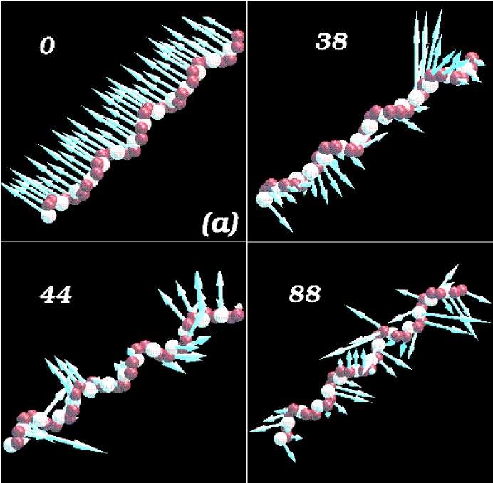
Figure 7:

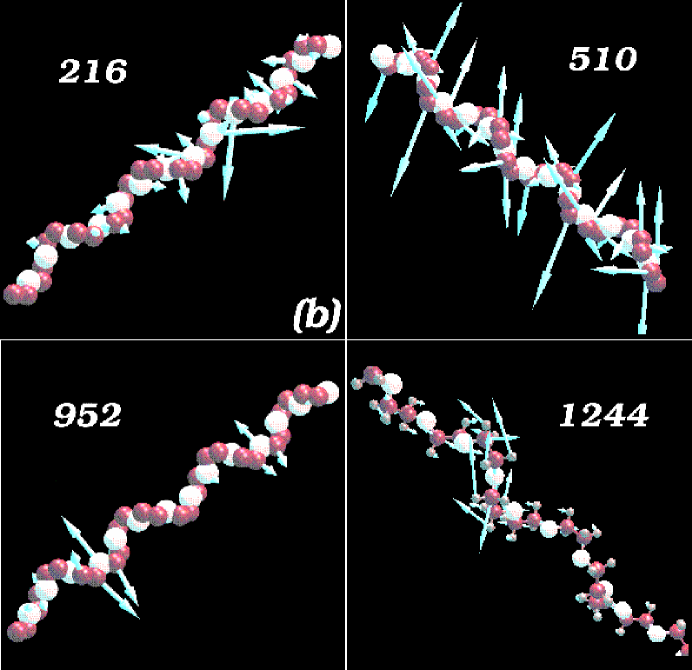
Figure 8:

Figure 4:    (a),(b) : Atomic displacements of representative normal modes of the PEO crystal. For each mode, one of the chains which exhibit significant atomic displacement is shown, for clarity. Red (or Black) spheres denote carbon atoms and white spheres denote oxygens. Hydrogen atoms are not shown for clarity in all the modes, except the one with frequency 1244 cm^-1. Arrows denote the directions of atomic displacements and their lengths are scaled up for the purpose of visualization. The mode at 0 cm^-1 is the rigid body translation of the chain, and that at 1244 cm^-1 arises from wagging of CH₂ groups. Frequencies in cm^-1 are as provided in the figures. The representation of these modes in the D₇ group, are as follows, with frequencies in cm^-1 given in paranthesis: A₂ (38), A₂ (44), E (88), A₁ (216), E (510), E (952), and E (1244).

Figure 9: Local character indicator for the normal modes of PEO crystal. The inset shows the frequency range where collective motion is most probable with very small local character indicator values.

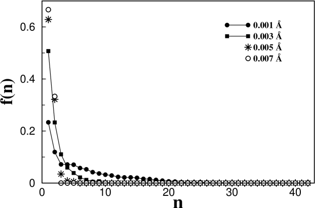
Figure 10: The segment size distribution, f(n), corresponding to the mode at 44 cm^-1 of the PEO crystal. The distribution is shown for four different displacement cutoffs. Such distributions are used to calculate the average continuous segment size ($<$CSS$>$) which is defined in equation (7).

Figure 11: Variation of the average continuous segment size ($<$CSS$>$) with respect to the vibrational frequencies for different displacement cutoffs.

References

- [1] J.W. Halley, and Y. Duan, J. Power Sources 89, 139 (2000).
- [2] M. Wakihara, Mat. Sci. Engg. R33, 109 (2001).
- [3] P.G. Bruce, Solid State Electrochemistry, Cambridge University Press, Cambridge, 1995.
- [4] P.G. Bruce, and C.A. Vincent, J. Chem. Soc. Faraday Trans. 89, 3187 (1993).
- [5] X.G. Sun, W. Xu, S.S. Zhang, and C.A. Angell, J. Phys. Cond. Matt. 13, 8235 (2001).
- [6] J.P. Donoso, T.J. Bonagamba, H.C. Panepucci, L.N. Oliveira, W. Gorecki, C. Berthier and M. Armand, J. Chem. Phys. 98, 10026 (1993).
- [7] I.M. Ward, N. Boden, J. Cruickshank, and S.A. Leng, Electrochim. Acta. 40, 2071 (1995).
- [8] G. Mao, R.F. Perea, W.S. Howells, D.L. Price, and M.-L. Saboungi, Nature (London) 405, 163 (2000); M.-L. Saboungi, D.L. Price, G. Mao, R.F. Perea, O. Borodin, and G.D. Smith, M. Armand, and W.S. Howells, Solid State Ionics 147, 225 (2002);
- [9] C.A. Angell, Solid State Ionics 9-10, 3 (1983).
- [10] C. Berthier, W. Gorecki, M. Minier, M.B. Armand, J.M. Chanbagno, and P. Rigaud, Solid State Ionics 11, 91 (1983).
- [11] W. Gorecki, P. Donoso, C. Berthier, M. Mali, J. Roos, D. Brinkmann, M.B. Armand, Solid State Ionics 28-30,1018 (1988).
- [12] Z. Gadjourova, Y.G. Andreev, D.P. Tunstall, and P.G. Bruce, Nature 412, 520 (2001)
- [13] B. Mos, P. Verkerk, A. van Zon, and S.W. de Leeuw, Physica B 276, 351 (2000); S.W. de Leeuw, A. Van Zon, and G.J. Bel, Electrochim. Acta 46, 1419 (2001); J.J. de Jonge, A. van Zon, and S.W. de Leeuw, Solid State Ionics 147, 349 (2002).
- [14] S. Neyertz, D. Brown, and J.O. Thomas, J. Chem. Phys. 101, 10064 (1994).
- [15] S. Neyertz, Ph.D. thesis, Uppsala University, Uppsala, 1995.
- [16] S. Neyertz, and D. Brown, J. Chem. Phys. 102, 9725 (1995).
- [17] S. Neyertz, D. Brown, and J.O. Thomas, Electrochim. Acta 40, 2063 (1995).
- [18] S. Neyertz, D. Brown, and J.O. Thomas, Comput. Polym. Sci. 5, 107 (1995).
- [19] F. Muller-Plathe, and W.F. van Gunsteren, J. Chem. Phys. 103, 4745 (1995).
- [20] K. Laasonen, and M.L. Klein, J. Chem. Soc. Faraday Trans. 91, 2633 (1995).
- [21] J.W. Halley, Y. Duan, B. Nielsen, P.C. Redfern, and L.A. Curtiss, J. Chem. Phys. 115, 3957 (2001); B. Lin, P.T. Boinske, and J.W. Halley, J. Chem. Phys. 105, 1668 (1996).
- [22] P. Ahlstrm, G. Wahnstrm, P. Carlsson, O. Borodin, and G.D. Smith, J. Chem. Phys. 112, 10669 (2000).
- [23] O. Borodin, and G.D. Smith, Macromolecules 31, 8396 (1998); Macromolecules 33, 2273 (2000);
- [24] O. Borodin, F. Trouw, D. Bedrov, and G.D. Smith, J. Phys. Chem. B 106, 5184 (2002); O. Borodin, D. Bedrov, and G.D. Smith, J. Phys. Chem. B 106, 5194 (2002); G.D. Smith, D. Bedrov, and O. Borodin, Phys. Rev. Lett. 85, 5583 (2000).
- [25] G.D. Smith, O. Borodin, M. Pekny, B. Annis, D. Londono, and R.L. Jaffe, Spectrochim. Acta A 53, 1273 (1997).
- [26] G. Carini, G. D’Angelo, G. Tripodo, A. Bartolotta, and G. Di Marco Phys. Rev. B 54, 15056-15063 (1996).
- [27] P. Mustarelli, C. Capiglia, E. Quartarone, C. Tomasi, P. Ferloni, and L. Linati, Phys. Rev. B 60, 7228 (1999).
- [28] S.I. Simdyankin, M. Dzugutov, S.N. Taraskin, and S.R. Elliott, Phys. Rev. B 63, 184301 (2001); S.N. Taraskin, and S.R. Elliott, Phys. Rev. B 61, 12017 (2000); S.N. Taraskin, and S.R. Elliott, Phys. Rev. B 59, 8572 (1999).
- [29] C.S. O’Hern, S.A. Langer, A.J. Liu, and S.R. Nagel, Phys. Rev. Lett. 86, 111 (2001).
- [30] K. Fukui, B.G. Sumpter, D.W. Noid, C. Yang, and R.E. Tuzun, J. Phys. Chem. B, 104, 526 (2000); D.W. Noid, K. Fukui, B.G. Sumpter, C. Yang, and R.E. Tuzun, Chem. Phys. Lett.316, 285 (2000).
- [31] H.W.T. van Vlijmen and M. Karplus, J. Phys. Chem. B 103, 3009 (1999).
- [32] N.P. Barton, C.S. Verma, L.S.D. Caves, J. Phys. Chem. B 107, 2170 (2003); J. Phys. Chem. B 106, 11036 (2002).
- [33] Y. Takahashi and H. Tadokoro, Macromolecules 6, 672 (1973).
- [34] G.J. Martyna, M.L. Klein, and M. Tuckerman, J. Chem. Phys. 97, 2635 (1992).
- [35] M.E. Tuckerman, D.A. Yarne, S.O. Samuelson, A.L. Hughes, and G. Martyna, Comput. Phys. Commun. 128, 333 (2000).
- [36] J.-P. Hansen, in Molecular Dynamics Simulations of Statistical Mechanics Systems, Ed. G. Ciccotti, and W.G. Hoover, (North-Holland, Amsterdam, 1986).
- [37] A.D. MacKerell Jr. et al, J. Phys. Chem. B 102, 3586 (1998).
- [38] M. Abramowitz, and I.A. Stegun, Handbook of Mathematical Functions, (Dover, New York, 1970).
- [39] S.N. Taraskin, and S.R. Elliott, Phys. Rev. B. 56, 8605 (1997).
- [40] M. Parrinello, and A. Rahman, Phys. Rev. Lett. 45, 1196 (1980).
- [41] J.F. Rabolt, K.W. Johnson, and R.N. Zitter, J. Chem. Phys. 61, 504, (1974).
- [42] V.M. Da Costa, T.G. Fiske, and L.B. Coleman, J. Chem. Phys. 101, 2746, (1994).
- [43] C. Branca, A. Faraone, S. Magazu, G. Maisano, P. Migliardo, and V. Villari, J. Mol. Liquids 87, 21 (2000).
- [44] T. Yoshihara, H. Tadokoro, S. Murahashi, J. Chem. Phys. 41, 2902 (1964).
- [45] K. Song, and S. Krimm, J. Polym. Sci. Polym. Phys. Ed. 28, 35, (1990).
- [46] D.A. Case, Curr. Opin. Struct. Biol. 4, 285 (1994).