Analytic calculation of $B_{4}$ for hard spheres in even dimensions

Abstract

We exactly calculate the fourth virial coefficient for hard spheres in even dimensions for $D=4,6,8,10,$ and 12.

Keywords: hard spheres, virial expansion.

1 Introduction

The virial series for the pressure

$$\frac{P}{k_{B}T}=\rho+\sum_{k=2}^{\infty}B_{k}\rho^{k}$$ (1)

of the system of hard spheres with diameter $\sigma$ in $D$ dimensions specified by the two body pair potential

$$U({\bf r})=\left\{\begin{array}[]{c}+\infty\\ 0\end{array}\right.\begin{array}[]{c}|{\bf r}|<\sigma\\ |{\bf r}|>\sigma\\ \end{array}$$ (2)

has been studied for over 100 years. However, despite the long history of this problem, there are very few analytic results known. The second virial coefficient is

$$B_{2}=\frac{\sigma^{D}\pi^{D/2}}{2\,\Gamma(1+D/2)}$$ (3)

The third virial coefficient has been computed long ago for $D=2$ [1] and $D=3$ [2], and in arbitrary dimension is compactly given as [3]

$$B_{3}/B_{2}^{2}=\frac{4\,\Gamma(1+\frac{D}{2})}{\pi^{1/2}\Gamma(\frac{1}{2}+\frac{D}{2})}\int_{0}^{\pi/3}d\phi\;(\sin\phi)^{D}$$ (4)

For low dimensions these are given in Table 1.

Table 1: The second and third virial coefficients as functions of dimension.

		$B_{3}/B_{2}^{2}$
$D$	$B_{2}$	Exact	Numerical
$1$	$\sigma$	$1$	$1$
$2$	${\pi\sigma^{2}/2}$	$\frac{4}{3}-{\frac{\sqrt{3}}{\pi}}$	$0.782004\cdots$
$3$	${2\pi\sigma^{3}/3}$	${5/8}$	$0.625$
$4$	${\pi^{2}\sigma^{4}/4}$	$\frac{4}{3}-\frac{\sqrt{3}}{\pi}\frac{3}{2}$	$0.506340\cdots$
$5$	${4\pi^{2}\sigma^{5}/15}$	$53/2^{7}$	$0.414063\cdots$
$6$	${\pi^{3}\sigma^{6}/12}$	$\frac{4}{3}-\frac{\sqrt{3}}{\pi}\frac{9}{5}$	$0.340941\cdots$
$7$	${8\pi^{3}\sigma^{7}/105}$	$289/2^{10}$	$0.282227\cdots$
$8$	${\pi^{4}\sigma^{8}/48}$	$\frac{4}{3}-\frac{\sqrt{3}}{\pi}\frac{279}{140}$	$0.234614\cdots$
$9$	${16\pi^{4}\sigma^{9}/945}$	$6413/2^{15}$	$0.195709\cdots$
$10$	$\pi^{5}\sigma^{10}/240$	$\frac{4}{3}-\frac{\sqrt{3}}{\pi}\frac{297}{140}$	$0.163728\cdots$
$11$	$32\pi^{5}\sigma^{11}/10395$	$35995/2^{18}$	$0.137310\cdots$
$12$	$\pi^{6}\sigma^{12}/1440$	$\frac{4}{3}-\frac{\sqrt{3}}{\pi}\frac{243}{110}$	$0.115398\cdots$

However, $B_{4}$ has been calculated analytically in only two and three dimensions

$$\frac{B_{4}}{B_{2}^{3}} = \left\{\begin{array}[]{ll}2-\frac{9\sqrt{3}}{2\pi}+\frac{10}{\pi^{2}}&{\rm for}\;D=2{\mbox{\cite[cite]{[\@@bibref{}{rowlinson1964a,hemmer1964a}{}{}]}}}\\ \frac{219\sqrt{2}}{2240\pi}-\frac{89}{280}+\frac{4131}{2240\pi}\arctan{\sqrt{2}}&{\rm for}\;D=3{\mbox{\cite[cite]{[\@@bibref{}{boltzmann1899a,vanlaar1899a,nijboer1952a}{}{}]}}}\end{array}\right.$$ (7)

and no further analytic results are known. An interesting discussion of the history of the calculation of $B_{4}$ in three dimensions is given in [8].

We feel that for such a problem in pure geometry that tractable analytic results must exist. In this paper we make a modest step toward verifying this by extending the analytic evaluation of the fourth virial coefficient to even dimensions $D\leq 12.$

In the Mayer formalism [9] the fourth virial coefficient is

$$B_{4}=-\frac{1}{8}\,\raisebox{-2.84544pt}{\includegraphics[height=11.38092pt]{mayer4c}}-\frac{3}{4}\,\raisebox{-2.84544pt}{\includegraphics[height=11.38092pt]{mayer4b}}-\frac{3}{8}\,\raisebox{-2.84544pt}{\includegraphics[height=11.38092pt]{mayer4a}}$$ (8)

where each solid line represents the Mayer $f$ function

$$f({\bf r})=\exp\left({-U({\bf r})/k_{B}T}\right)-1$$ (9)

which for the hard sphere potential reduces to

$$f({\bf r})=\left\{\begin{array}[]{r}-1\\ 0\end{array}\right.\begin{array}[]{l}|{\bf r}|<\sigma\\ |{\bf r}|>\sigma\\ \end{array}$$ (10)

The second and third diagrams in this expansion have been evaluated in arbitrary dimension in [3, 10]. In this paper we complete the computation in even dimensions for $D\leq 12$ by evaluating the first diagram in Section 2.

For virial coefficients of order greater than four it is much more efficient to use the expansion of Ree and Hoover [11, 12] where in addition to the $f$ bonds we also have bonds ${\tilde{f}}({\bf r})=1+f({\bf r})$ which are represented by dotted lines. In this notation every point is connected to every other point by either an $f$ or an ${\tilde{f}}$ bond and for $B_{4}$ the virial coefficient is given by

$$B_{4}=\frac{1}{4}\,\emptyset-\frac{3}{8}\,\raisebox{-2.84544pt}{\includegraphics[height=11.38092pt]{wiggly2}}$$ (11)

where only the $\tilde{f}$ bonds are shown. The integral in the first term is identical with the integral in the first term of Eq. 8 and we compute the second term from the three Mayer diagrams of Eq. 8 in Section 3. The results for $B_{4}$ and for the two separate Ree-Hoover diagrams are given in Table 2.

Table 2: Analytical results for the four point Ree-Hoover diagrams and $B_{4}$ in even dimensions, with numerical values.

$D$	$\emptyset/B_{2}^{3}$	$\raisebox{-2.84544pt}{\includegraphics[height=11.38092pt]{wiggly2}}/B_{2}^{3}$	$B_{4}/B_{2}^{3}$
2	$8-\frac{12\sqrt{3}}{\pi}+\frac{8}{\pi^{2}}$	$\frac{4\sqrt{3}}{\pi}-\frac{64}{3\pi^{2}}$	$2-\frac{9\sqrt{3}}{2\pi}+\frac{10}{\pi^{2}}$
	$2.194622724\cdots$	$0.043796999\cdots$	$0.532231807\cdots$
4	$8-\frac{18\sqrt{3}}{\pi}+\frac{238}{9\pi^{2}}$	$\frac{6\sqrt{3}}{\pi}-\frac{4276}{135\pi^{2}}$	$2-\frac{27\sqrt{3}}{4\pi}+\frac{832}{45\pi^{2}}$
	$0.755462293\cdots$	$0.098718698\cdots$	$0.151846062\cdots$
6	$8-\frac{108\sqrt{3}}{5\pi}+\frac{37259}{900\pi^{2}}$	$\frac{36\sqrt{3}}{5\pi}-\frac{72151}{1890\pi^{2}}$	$2-\frac{81\sqrt{3}}{10\pi}+\frac{38848}{1575\pi^{2}}$
	$0.285880282\cdots$	$0.101618460\cdots$	$0.033363148\cdots$
8	$8-\frac{837\sqrt{3}}{35\pi}+\frac{5765723}{110250\pi^{2}}$	$\frac{279\sqrt{3}}{35\pi}-\frac{77417239}{1819125\pi^{2}}$	$2-\frac{2511\sqrt{3}}{280\pi}+\frac{17605024}{606375\pi^{2}}$
	$0.114137690\cdots$	$0.082912284\cdots$	$-0.002557687\cdots$
10	$8-\frac{891\sqrt{3}}{35\pi}+\frac{41696314}{694575\pi^{2}}$	$\frac{297\sqrt{3}}{35\pi}-\frac{1044625732}{22920975\pi^{2}}$	$2-\frac{2673\sqrt{3}}{280\pi}+\frac{49048616}{1528065\pi^{2}}$
	$0.047194685\cdots$	$0.06069639\cdots$	$-0.01096248\cdots$
12	$8-\frac{1458\sqrt{3}}{55\pi}+\frac{88060381669}{1344697200\pi^{2}}$	$\frac{486\sqrt{3}}{55\pi}-\frac{21249584434511}{445767121800\pi^{2}}$	$2-\frac{2187\sqrt{3}}{220\pi}+\frac{11565604768}{337702365\pi^{2}}$
	$0.020007319\cdots$	$0.041792298\cdots$	$-0.010670281\cdots$

2 Analytical Calculation of the Complete Star Diagram

The complete star integral in the expansions of Eq. 8 and Eq. 11 is by definition

$$= \lim_{V\rightarrow\infty}\frac{1}{V}\int d^{D}{\bf r_{1}}d^{D}{\bf r_{2}}d^{D}{\bf r_{3}}d^{D}{\bf r_{4}}f({\bf r_{12}})f({\bf r_{13}})f({\bf r_{14}})f({\bf r_{23}})f({\bf r_{24}})f({\bf r_{34}})$$ (12)

$$= \int d^{D}{\bf r_{1}}d^{D}{\bf r_{2}}d^{D}{\bf r_{3}}f({\bf r_{12}})f({\bf r_{13}})f({\bf r_{23}})f({\bf r_{1}})f({\bf r_{2}})f({\bf r_{3}})$$

where ${\bf r_{ij}}={\bf r_{i}-r_{j}}.$ Specializing to the case of hard spheres we first note that $f({\bf r})\equiv f(|{\bf r}|)$, and then we treat the coordinates in Eq. 12 as follows: ${\bf r_{1}}$ is constrained to a unit ball centered on the origin due to $f(r_{1})$, ${\bf r_{2}}$ is integrated in the same ball with the additional condition that $r_{12}\equiv|{\bf r_{12}}|=\sqrt{r_{1}^{2}+r_{2}^{2}-2r_{1}r_{2}\cos\theta}<1$. The ${\bf r_{3}}$ integral may be thought of as giving the overlapping hypervolume $V_{D}$ of $D$–dimensional unit balls situated at the origin, ${\bf r_{1}}$, and ${\bf r_{2}}$, and this depends only on $r_{1}$, $r_{2}$, and the angle $\theta$ between ${\bf r_{1}}$ and ${\bf r_{2}}$. We define $V_{D}$ as

$$V_{D}(r_{1},r_{2},\theta)=-\int d^{D}{\bf r_{3}}f({\bf r_{13}})f({\bf r_{23}})f({\bf r_{3}})$$ (13)

where the negative sign ensures that $V_{D}$ is positive. We may substitute this in to the expression for , and then write ${\bf r_{1}}$ and ${\bf r_{2}}$ in $D$–dimensional spherical polar coordinates

$$= -\int d^{D}{\bf r_{1}}d^{D}{\bf r_{2}}f(r_{1})f(r_{2})f(r_{12})V_{D}(r_{1},r_{2},\theta)$$ (14)

$$= -\int dr_{1}r_{1}^{D-1}\int d\Omega_{D-1}^{(1)}\int dr_{2}r_{2}^{D-1}\int d\theta(\sin\theta)^{D-2}\int d\Omega_{D-2}^{(2)}$$

$$\times f(r_{1})f(r_{2})f(r_{12})V_{D}(r_{1},r_{2},\theta)$$

where the angular integrals give $\Omega_{D-1}\equiv\int d\Omega_{D-1}=2\pi^{D/2}/\Gamma(D/2)$, which is valid for arbitrary $D>0$, including non-integer $D$. The integrand in Eq. 14 only depends on $r_{1}$, $r_{2}$, and $\theta$, and we may integrate out the other angles to obtain

$$= -\Omega_{D-1}\Omega_{D-2}\int dr_{1}r_{1}^{D-1}\int dr_{2}r_{2}^{D-1}\int d\theta(\sin\theta)^{D-2}$$ (15)

$$\times f(r_{1})f(r_{2})f(r_{12})V_{D}(r_{1},r_{2},\theta)$$

We now change coordinates from $(r_{1},r_{2},\theta)$ to the coordinate system $(R,\alpha,\beta)$ which is illustrated in Fig. 2. The three points which were at the origin, ${\bf r_{1}}$, and ${\bf r_{2}}$ are now circumscribed by a circle of radius $R$; $2\alpha$ and $2\beta$ are the angles subtended by $r_{1}$ and $r_{2}$ from the center of the circle.

$$r_{1} = 2R\sin\alpha$$

$$r_{2} = 2R\sin\beta$$

$$\theta = \pi-\alpha-\beta$$ (16)

Noting also that $-f(r_{1})f(r_{2})f(r_{12})$ may only have the values of 0 and 1, we may absorb the $f$ functions in to the domain of integration and rewrite the triple integral of Eq. 15 as

$$4^{D}\int d\alpha\int d\beta\int dRR^{2D-1}\left[\sin\alpha\sin\beta\sin(\alpha+\beta)\right]^{D-1}V_{D}(R,\alpha,\beta)$$ (17)

Figure 1: Change of variables.

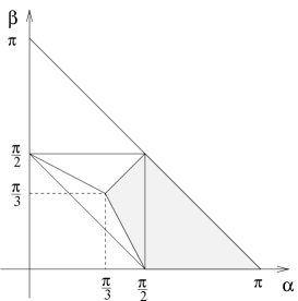
Figure 2: Domain of integration for $B_{4}$, where the shaded region satisfies the condition $\alpha>\beta,\gamma$.

We are required to integrate over all $R$, $\alpha$, and $\beta$ such that the distance between any two points is less than one; denoting the sides opposite points A, B, and C on Fig. 2 as a, b, and c respectively we have $a=2R\sin\alpha$, $b=2R\sin\beta$, and $c=2R\sin\gamma$. We choose to integrate over $R$ before the angles $\alpha$ and $\beta$, and we impose $b,c<a<1$ which introduces an extra factor of $3$. Therefore we must change the region of integration from

$$0< b< a$$ (18)

$$0< c< a$$ (19)

$$0< a< 1$$ (20)

to a domain for $(R,\alpha,\beta)$. The boundary of this region is found by setting inequalities 18 and 19 to equality, with solutions:

$$\alpha = \beta$$

$$\alpha = \pi-\beta$$

$$\alpha = \gamma\Rightarrow\beta=\pi-2\alpha$$

$$\alpha = \pi-\gamma\Rightarrow\beta=0$$ (21)

This region is shown in Fig. 2. Finally, inequality 20 restricts $R$ to the domain

$$0<R<\frac{1}{2\sin\alpha}$$ (22)

The next step is to calculate the overlapping volume $V_{D}$ of the three hyperspheres for even dimensions $D=2n$, where $n$ is an integer greater than or equal to 2. We do this in Appendix A, and the result for $R<1$ is denoted $V_{D}^{<}$ and given in Eq. 42, while the result for $R>1$ is denoted $V_{D}^{>}$ and given in Eq. 43. Throughout this paper we will adopt the convention that sums with index $\xi$ are always over $\{\alpha,\beta,\gamma\}$.

We will sketch the steps involved in the rest of the calculation, which were carried out using the computer algebra platform MAPLE version 8 for $n=2,3,4,5,6$. The first step is to perform the integral over $R$, where we notice from inequality 22 that we may only have $R>1$ when $\alpha>\frac{5\pi}{6}$. Ignoring for the moment factors not involving $R$ in Eq. 17, we therefore need to calculate

$$I_{2}=\int_{0}^{1/2\sin\alpha}dR\;R^{4n-1}V_{D}^{<}\quad\alpha<\frac{5\pi}{6}$$ (23)

and

$$I_{3}=\int_{0}^{1}dR\;R^{4n-1}V_{D}^{<}+\int_{1}^{1/2\sin\alpha}dR\;R^{4n-1}V_{D}^{>}\quad\alpha>\frac{5\pi}{6}$$ (24)

One of the integrals we will need to do is

$$\int dR\;R^{4n-1}\left(\arccos(R\sin\xi)-R\sin\xi\ \sqrt{1-R^{2}\sin^{2}\xi}\right)$$

$$=\frac{1}{4n}R^{4n}\left(\arccos(R\sin\xi)-R\sin\xi\ \sqrt{1-R^{2}\sin^{2}\xi}\right)$$

$$+\frac{1}{2n}\int dR\;R^{4n}\sin\xi\ \sqrt{1-R^{2}\sin^{2}\xi}$$ (25)

and thus the only non-trivial parts of the integral are in the form $\int dR\;R^{2l}U^{m+\frac{1}{2}}$ with the shorthand notation $U=1-R^{2}\sin^{2}\xi$. We substitute
$R^{2}=[{1-(1-R^{2}\sin^{2}\xi)}]/{\sin^{2}\xi}$ everywhere, and this leaves us only to perform integrals such as

$$\int dR\;U^{j+\frac{1}{2}} = \frac{\sqrt{U}}{2(j+1)}\left\{U^{j}+\sum_{k=0}^{j-1}\frac{(2j+1)(2j-1)\ldots(2j-2k+1)}{2^{k+1}j(j-1)\ldots(j-k)}U^{j-k-1}\right\}$$ (26)

$$+\frac{(2n+1)!!\arcsin(R\sin\xi)}{2^{j+1}(j+1)!\sin\xi}$$

We may replace $\gamma$ everywhere in this expression by $\beta$, as we are integrating over a region that is symmetric in $\beta$ and $\gamma$. After doing this and substituting in the limits of integration, we are left with terms involving $[{1-\sin^{2}\beta/(4\sin^{2}\alpha)}]^{1/2}$ and $\arcsin[\sin\beta/(2\sin\alpha)]$, along with functions of the form $x^{-m}P(x)$ where $m$ is an integer, $P(x)$ is a polynomial, and $x$ may be either $\sin\alpha$ or $\sin\beta$. We now make the change of variables $x=\sin\alpha$, $y=\sin\beta$, and so the $\alpha$ and $\beta$ integrals become

$$\int d\alpha\int d\beta\;\left[\sin\alpha\sin\beta\sin(\alpha+\beta)\right]^{2n-1}$$

$$= \int dx\;\frac{1}{\sqrt{1-x^{2}}}\int dy\;\frac{1}{\sqrt{1-y^{2}}}\;x^{2n-1}y^{2n-1}\left[x\sqrt{1-y^{2}}\pm y\sqrt{1-x^{2}}\right]^{2n-1}$$

$$= \int dx\;\frac{x^{2n-1}}{\sqrt{1-x^{2}}}\int dy\;\frac{y^{2n-1}}{\sqrt{1-y^{2}}}\sum_{j=0}^{2n-1}{2n-1\choose j}\left[x\sqrt{1-y^{2}}\right]^{j}\left[\pm y\sqrt{1-x^{2}}\right]^{2n-1-j}$$

$$= \sum_{j=0}^{n-1}{2n-1\choose j}\int dx\;x^{2n-1}\int dy\;y^{2n-1}\left[\pm\frac{\left[x^{2}(1-y^{2})\right]^{j}\left[y^{2}(1-x^{2})\right]^{n-1-j}\;y}{\sqrt{1-y^{2}}}\right.$$

$$\left.+\frac{\left[y^{2}(1-x^{2})\right]^{j}\left[x^{2}(1-y^{2})\right]^{n-1-j}\;x}{\sqrt{1-x^{2}}}\right]$$

The ambiguous sign is $+$ when $\alpha<\frac{\pi}{2}$ and $-$ when $\alpha>\frac{\pi}{2}$. Under the change of coordinates $[1-\sin^{2}\beta/(4\sin^{2}\alpha)]^{1/2}$ becomes $[4x^{2}-y^{2}]^{1/2}/(2x)$, and so naively it appears that we have to compute elliptic integrals of the form $\int dz\sqrt{t^{2}-z^{2}}/{\sqrt{1-z^{2}}}$ and then use identities for elliptic integrals to reduce the final result to a simple form. However, by splitting the final integrals over x and y for  in to the pieces

$$\pm\int dx\;x^{2n-1}\int\;dyy^{2n-1}\left[x^{2}(1-y^{2})\right]^{j}\left[y^{2}(1-x^{2})\right]^{n-1-j}\frac{y}{\sqrt{1-y^{2}}}\;(I_{2}\ \mathrm{or}\ I_{3})$$

$$+\int dx\;x^{2n-1}\int dy\;y^{2n-1}\left[y^{2}(1-x^{2})\right]^{j}\left[x^{2}(1-y^{2})\right]^{n-1-j}\frac{x}{\sqrt{1-x^{2}}}\;(I_{2}\ \mathrm{or}\ I_{3})$$

we avoid this. The first integral may be completed straightforwardly by first integrating over x, and then when one substitutes in the limits of integration this eliminates any elliptic integrals. The integral over y may now be performed without requiring any elliptic functions. Conversely, the second integral is completed by first integrating over y and subsequently over x. Thus one can see that for any even dimension all integrals that must be performed are elementary.

So we obtain the results of Table 2 by carrying out this procedure for $D=4,6,8,10,$ and $12$ using MAPLE.

3 Analytic derivation of the Ree-Hoover ring diagram

The second and third Mayer diagrams have been found in terms of integrals over Bessel functions and hypergeometric functions by Luban and Baram [3]. The Mayer ring diagram is given by

$$\raisebox{-2.84544pt}{\includegraphics[height=11.38092pt]{mayer4a}}=\frac{2^{D+4}}{\pi}\frac{\Gamma(1+D)\left[\Gamma(1+\frac{D}{2})\right]^{3}}{\Gamma(1+\frac{3D}{2})\left[\Gamma(\frac{3}{2}+\frac{D}{2})\right]^{2}}\;{}_{3}F_{2}\left(\frac{1}{2},1,\frac{1-D}{2};\frac{3+D}{2},\frac{3+D}{2};1\right)$$

while the second Mayer diagram is given in [3] as

$$\raisebox{-2.84544pt}{\includegraphics[height=11.38092pt]{mayer4b}}=-2^{D+1}D^{3}[\Gamma(D/2)]^{2}\int_{0}^{2}dy\;y\left[g_{D/2}(y)\right]^{2}$$

where

$$g_{\nu}(y)=\int_{0}^{\infty}dx\;x^{-\nu}\left[J_{\nu}(x)\right]^{2}J_{\nu-1}(xy)$$

Other expressions for these diagrams were given in [3, 10], but MAPLE was straightforwardly able to evaluate these expressions for dimensions one through twelve, and these are listed Table 3. The second diagram of the Ree-Hoover expansion was then obtained from the equation

$$\raisebox{-2.84544pt}{\includegraphics[height=11.38092pt]{wiggly2}}=\raisebox{-2.84544pt}{\includegraphics[height=11.38092pt]{mayer4c}}+2\;\raisebox{-2.84544pt}{\includegraphics[height=11.38092pt]{mayer4b}}+\raisebox{-2.84544pt}{\includegraphics[height=11.38092pt]{mayer4a}}$$ (27)

Table 3: $\raisebox{-2.84544pt}{\includegraphics[height=11.38092pt]{mayer4b}}/B_{2}^{3}$ and $\raisebox{-2.84544pt}{\includegraphics[height=11.38092pt]{mayer4a}}/B_{2}^{3}$ in dimensions up to twelve.

$D$	$\raisebox{-2.84544pt}{\includegraphics[height=11.38092pt]{mayer4b}}/B_{2}^{3}$	$\raisebox{-2.84544pt}{\includegraphics[height=11.38092pt]{mayer4a}}/B_{2}^{3}$
$1$	$-\frac{14}{3}$	$\frac{16}{3}$
$2$	$-8+\frac{8\sqrt{3}}{\pi}+\frac{20}{3\pi^{2}}$	$8-\frac{128}{3\pi^{2}}$
$3$	$-\frac{6347}{3360}$	$\frac{272}{105}$
$4$	$-8+\frac{12\sqrt{3}}{\pi}+\frac{173}{135\pi^{2}}$	$8-\frac{8192}{135\pi^{2}}$
$5$	$-\frac{20830913}{24600576}$	$\frac{4016}{3003}$
$6$	$-8+\frac{72\sqrt{3}}{5\pi}-\frac{193229}{37800\pi^{2}}$	$8-\frac{65536}{945\pi^{2}}$
$7$	$-\frac{87059799799}{217947045888}$	$\frac{296272}{415701}$
$8$	$-8+\frac{558\sqrt{3}}{35\pi}-\frac{76667881}{7276500\pi^{2}}$	$8-\frac{134217728}{1819125\pi^{2}}$
$9$	$-\frac{332647803264707}{1711029608251392}$	$\frac{1234448}{3187041}$
$10$	$-8+\frac{594\sqrt{3}}{35\pi}-\frac{9653909}{654885\pi^{2}}$	$8-\frac{1744830464}{22920975\pi^{2}}$
$11$	$-\frac{865035021570458459}{8949618140032008192}$	$\frac{55565456}{260468169}$
$12$	$-8+\frac{972\sqrt{3}}{55\pi}+\frac{182221984415}{10188962784\pi^{2}}$	$8-\frac{4312147165184}{55720890225\pi^{2}}$

Appendix A Calculation of $V_{D}$ in even dimensions

For $D=2$ the calculation of $V_{D}$ is straightforward as the ${\bf r_{3}}$ integral is confined to the same plane as the three circle centers and trivially gives the area of intersection of the three circles of radius $r=1$. Although we will neglect the details for the moment, the area depends on $R$, $\alpha$, and $\beta$ and we will denote this as $A(r=1,R,\alpha,\beta)$.

As shown in Fig. 3, for $D=3$, we define the perpendicular distance from the plane of the circle centers to be $h$; $h=0$ is the original plane in which we see three intersecting circles of radius one. As we increase $h$ we see overlapping circles with the same center but decreasing radius, with the radii of these circles given by $r=\sqrt{1-h^{2}}$ (see Figs. 5 and 5). The total volume of intersection may be obtained by integrating the overlapping area of the three circles with respect to $h$, from $h=0$ to the value $h_{\mathrm{max}}$ where the intersection of the three circles is reduced to a single point. There is an additional factor of two because we need to integrate both above and below the plane.

$$V_{3}(R,\alpha,\beta) = 2\int_{0}^{h_{\mathrm{max}}}dhA(r,R,\alpha,\beta)|_{r=\sqrt{1-h^{2}}}$$ (28)

$$= 2\int_{r_{\mathrm{min}}}^{1}dr\;\frac{r}{\sqrt{1-r^{2}}}A(r,R,\alpha,\beta)$$

Figure 3: Intersecting three dimensional spheres.

Figure 4: Circles produced by cutting intersecting spheres at $h=0$, $h={1}/{\sqrt{2}}$, and $h=\sqrt{1-R^{2}}={\sqrt{3}}/{2}$, where circle centers form an acute angled triangle.

Figure 5: Circles produced by cutting the intersecting spheres at $h=0$, $h={1}/{\sqrt{2}}$, and $h=\sqrt{1-R^{2}}={\sqrt{3}}/{2}$. In this case the circle centers form a triangle with an obtuse angle and the area of intersection will be non-zero even for $h>\sqrt{1-R^{2}}$.

For the general case of $D>3$, we choose a spherical polar coordinate system for the $D-2$ dimensional subspace with radial coordinate $h$; there is an extra factor of $h^{D-3}$ compared to three dimensional case, and we now need to perform an additional trivial angular integration, ie

$$V_{D}(R,\alpha,\beta) = \int_{0}^{h_{\mathrm{max}}}dhh^{D-3}\int d\Omega_{D-3}A(r,R,\alpha,\beta)|_{r=\sqrt{1-h^{2}}}$$ (29)

$$= \Omega_{D-3}\int_{0}^{h_{\mathrm{max}}}dhh^{D-3}A(r,R,\alpha,\beta)|_{r=\sqrt{1-h^{2}}}$$

$$= \Omega_{D-3}\int_{r_{\mathrm{min}}}^{1}dr\;r(1-r^{2})^{{(D-4)}/{2}}A(r,R,\alpha,\beta)$$

Although Eq. 29 breaks down for $D\leq 2$, note that it is correct for $D=3$ as $\Omega_{0}=2$.

As the area of intersection may be bounded by arcs from either two or three circles, we will need to deal with two different expressions for the area, and three different cases for $V_{D}$. In Fig. 3 we have $R<1$ and $\alpha<\frac{\pi}{2}$ in which case the area is bounded by three arcs over the full range of $r$, while in Fig. 5 we have $R<1$ and $\alpha>\frac{\pi}{2}$ for which the area is bounded by three arcs for $R<r<1$, but by two arcs for $R\sin\alpha<r<R$. When $R>1$ the area can only have two arcs for its boundary, and this is the third case.

Provided the overlapping region is bounded by arcs from three circles, the area of overlap may be calculated by an inclusion-exclusion method following the method used for the overlapping volume of 3 spheres in [13]. The area of intersection of three circles of radius r is given by

$$A^{(3)}(r,R,\alpha,\beta)$$ (30)

$$= (\mathrm{Area\ of\ }\bigtriangleup ABC)-\sum_{A_{i}=\{A,B,C\}}(\mathrm{Area\ of\ sector\ within\ circle\ A_{i}})$$

$$+\frac{1}{2}\sum_{\{A_{i},A_{j}\}}(\mathrm{Area\ of\ intersection\ of\ circles\ A_{i}\ and\ A_{j}})$$

$$= \frac{1}{2}R^{2}(\sin 2\alpha+\sin 2\beta+\sin 2\gamma)-\frac{1}{2}r^{2}(\alpha+\beta+\gamma)$$

$$+\sum_{\xi}\left(r^{2}\arccos\left(\frac{R\sin\xi}{r}\right)-R\sin\xi\ \sqrt{r^{2}-R^{2}\sin^{2}\xi}\right)$$

$$= R^{2}\sum_{\xi}\sin\xi\cos\xi\;-\frac{1}{2}\pi r^{2}$$

$$+\sum_{\xi}\left(r^{2}\arccos\left(\frac{R\sin\xi}{r}\right)-R\sin\xi\ \sqrt{r^{2}-R^{2}\sin^{2}\xi}\right)$$

The different contributions to Eq. 30 are shown explicitly in Fig. 6, and one should also note that although expressions are written in terms of $\alpha$, $\beta$, and $\gamma$ for the sake of simplicity, these variables are not independent and $\alpha+\beta+\gamma=\pi$.

Figure 6: The different kinds of contributions to the inclusion-exclusion formula for the area of intersection of three circles: (a) Area of $\bigtriangleup ABC$ (b) Area of sector A (c) Half of the area of intersection of circles A and B.

The overlap of two circles of radius r separated by a distance $R\sin\alpha$ is given by

$$A^{(2)}(r,R,\alpha)=2\left(r^{2}\arccos\left(\frac{R\sin\alpha}{r}\right)-R\sin\alpha\ \sqrt{r^{2}-R^{2}\sin^{2}\alpha}\ \right)$$ (31)

We may obtain this expression from Eq. 30 by taking the limit $r\rightarrow R^{+}$ when $\alpha>\frac{\pi}{2}$. Thus the three expressions for $V_{D}$ are

$$\frac{V_{D}}{\Omega_{D-3}} = \int_{R}^{1}dr\;r\,(1-r^{2})^{{(D-4)}/{2}}A^{(3)}\quad\alpha<\frac{\pi}{2}$$ (32)

$$\frac{V_{D}}{\Omega_{D-3}} = \int_{R}^{1}dr\;r\,(1-r^{2})^{{(D-4)}/{2}}A^{(3)}$$ (33)

$$+\int_{R\sin\alpha}^{R}dr\;r\,(1-r^{2})^{{(D-4)}/{2}}A^{(2)}\quad\alpha>\frac{\pi}{2}\ R<1$$

$$\frac{V_{D}}{\Omega_{D-3}} = \int_{R\sin\alpha}^{1}dr\;r\,(1-r^{2})^{{(D-4)}/{2}}A^{(2)}\quad\alpha>\frac{\pi}{2}\ R>1$$ (34)

We will now specialize to the case where $D=2n$, where $n$ is an integer greater than or equal to $2$. By defining

$$I_{1}(r,\xi) \equiv \int_{0}^{r}dr\;r^{3}(1-r^{2})^{n-2}\left[\arccos\left(\frac{R\sin\xi}{r}\right)-\frac{R\sin\xi}{r}\sqrt{1-\left(\frac{R\sin\xi}{r}\right)^{2}}\right]$$

and integrating out the remaining pieces, we have for $\alpha<{\pi}/{2}$, $R<1$:

$$\frac{V_{D}}{\Omega_{D-3}} = \int_{R}^{1}dr\;r(1-r^{2})^{n-2}\left[R^{2}\sum_{\xi}\sin\xi\cos\xi\;-\frac{1}{2}\pi r^{2}\right]$$

$$+\sum_{\xi}\left(I_{1}(1,\xi)-I_{1}(R,\xi)\right)$$

$$= -\frac{(1-R^{2})^{n-1}}{2(n-1)}R^{2}\sum_{\xi}\sin\xi\cos\xi\;+\left(\frac{(1-R^{2})^{n}}{2n}-\frac{(1-R^{2})^{n-1}}{2(n-1)}\right)\frac{\pi}{2}$$

$$+\sum_{\xi}\left(I_{1}(1,\xi)-I_{1}(R,\xi)\right)$$

while for $\alpha>{\pi}/{2}$, $R<1$:

$$\frac{V_{D}}{\Omega_{D-3}} = -\frac{(1-R^{2})^{n-1}}{2(n-1)}R^{2}\sum_{\xi}\sin\xi\cos\xi\;+\left(\frac{(1-R^{2})^{n}}{2n}-\frac{(1-R^{2})^{n-1}}{2(n-1)}\right)\frac{\pi}{2}$$

$$+\sum_{\xi}\left(I_{1}(1,\xi)-I_{1}(R,\xi)\right)+2(I_{1}(R,\alpha)-I_{1}(R\sin\alpha,\alpha))$$

$$= -\frac{(1-R^{2})^{n-1}}{2(n-1)}R^{2}\sum_{\xi}\sin\xi\cos\xi\;+\left(\frac{(1-R^{2})^{n}}{2n}-\frac{(1-R^{2})^{n-1}}{2(n-1)}\right)\frac{\pi}{2}$$

$$+\sum_{\xi}I_{1}(1,\xi)+I_{1}(R,\alpha)-I_{1}(R,\beta)-I_{1}(R,\gamma)-2I_{1}(R\sin\alpha,\alpha))$$

and finally for $\alpha>\frac{\pi}{2}$, $R>1$:

$$\frac{V_{D}}{\Omega_{D-3}} = 2(I_{1}(1,\alpha)-I_{1}(R\sin\alpha,\alpha))$$

Integrating $I_{1}$ once by parts

$$I_{1}(r,\xi) = \left[\frac{(1-r^{2})^{n-2}}{2n}-\frac{(1-r^{2})^{n-1}}{2(n-1)}+\frac{1}{2n(n-1)}\right]$$ (35)

$$\times\left[\arccos\left(\frac{R\sin\xi}{r}\right)-\frac{R\sin\xi}{r}\sqrt{1-\left(\frac{R\sin\xi}{r}\right)^{2}}\right]$$

$$-\sum_{j=0}^{n-2}\frac{(-1)^{j}}{j+2}{n-2\choose j}\int_{0}^{r}dr\;r^{2j+1}R\sin\xi\ \sqrt{r^{2}-R^{2}\sin^{2}\xi}$$

$$= \left[\frac{(1-r^{2})^{n-2}}{2n}-\frac{(1-r^{2})^{n-1}}{2(n-1)}+\frac{1}{2n(n-1)}\right]$$

$$\times\left[\arccos\left(\frac{R\sin\xi}{r}\right)-\frac{R\sin\xi}{r}\sqrt{1-\left(\frac{R\sin\xi}{r}\right)^{2}}\right]$$

$$-\sum_{j=0}^{n-2}\frac{(-1)^{j}}{j+2}{n-2\choose j}$$

$$\times\int_{0}^{r}dr\;r((r^{2}-R^{2}\sin^{2}\xi)+R^{2}\sin^{2}\xi)^{j}R\sin\xi\ \sqrt{r^{2}-R^{2}\sin^{2}\xi}$$

$$= \left[\frac{(1-r^{2})^{n-2}}{2n}-\frac{(1-r^{2})^{n-1}}{2(n-1)}+\frac{1}{2n(n-1)}\right]$$

$$\times\left[\arccos\left(\frac{R\sin\xi}{r}\right)-\frac{R\sin\xi}{r}\sqrt{1-\left(\frac{R\sin\xi}{r}\right)^{2}}\right]$$

$$-\sum_{j=0}^{n-2}\sum_{k=0}^{j}\frac{(-1)^{j}}{j+2}{n-2\choose j}{j\choose k}(R\sin\xi)^{2j-2k+1}$$

$$\times\int_{0}^{r}dr\;r(r^{2}-R^{2}\sin^{2}\xi)^{k+\frac{1}{2}}$$

$$= \left[\frac{(1-r^{2})^{n-2}}{2n}-\frac{(1-r^{2})^{n-1}}{2(n-1)}+\frac{1}{2n(n-1)}\right]$$

$$\times\left[\arccos\left(\frac{R\sin\xi}{r}\right)-\frac{R\sin\xi}{r}\sqrt{1-\left(\frac{R\sin\xi}{r}\right)^{2}}\right]$$

$$-\sum_{j=0}^{n-2}\sum_{k=0}^{j}\frac{(-1)^{j}}{j+2}{n-2\choose j}{j\choose k}(R\sin\xi)^{2j-2k+1}$$

$$\times\frac{(r^{2}-R^{2}\sin^{2}\xi)^{k+\frac{3}{2}}}{2k+3}$$

where we have used

$$\int_{0}^{r}dr\;r^{3}(1-r^{2})^{n-2} = \int_{0}^{r}dr\;r(1-(1-r^{2}))(1-r^{2})^{n-2}$$ (36)

$$= -\frac{(1-r^{2})^{n-1}}{2(n-1)}+\frac{(1-r^{2})^{n}}{2n}+\frac{1}{2n(n-1)}$$

$$= \frac{1}{2}\sum_{j=0}^{n-2}\frac{(-1)^{j}}{j+2}{n-2\choose j}r^{2j+4}$$

and

$$\frac{d}{dr}\left[\arccos\left(\frac{R\sin\xi}{r}\right)-\frac{R\sin\xi}{r}\sqrt{1-\left(\frac{R\sin\xi}{r}\right)^{2}}\right]$$ (37)

$$= \frac{2R\sin\xi}{r^{2}}\sqrt{1-\left(\frac{R\sin\xi}{r}\right)^{2}}$$

Substituting in the limits of integration, $r=1$

$$I_{1}(1,\xi) = \frac{1}{2n(n-1)}\left[\arccos(R\sin\xi)-R\sin\xi\ \sqrt{1-R^{2}\sin^{2}\xi}\right]$$ (38)

$$-\sum_{j=0}^{n-2}\sum_{k=0}^{j}\frac{(-1)^{j}}{j+2}{n-2\choose j}{j\choose k}(R\sin\xi)^{2j-2k+1}\frac{(1-R^{2}\sin^{2}\xi)^{k+\frac{3}{2}}}{2k+3}$$

Substituting $r=R$

$$I_{1}(R,\xi) = \left[\frac{(1-R^{2})^{n-2}}{2n}-\frac{(1-R^{2})^{n-1}}{2(n-1)}+\frac{1}{2n(n-1)}\right]$$ (39)

$$\times\left[\arccos(\sin\xi)-\sin\xi\sqrt{\cos^{2}\xi}\right]$$

$$-\sum_{j=0}^{n-2}\sum_{k=0}^{j}\frac{(-1)^{j}}{j+2}{n-2\choose j}{j\choose k}(R\sin\xi)^{2j-2k+1}\frac{R^{2k+3}(\cos^{2}\xi)^{k+\frac{3}{2}}}{2k+3}$$

$$= \mathrm{sgn}\left(\frac{\pi}{2}-\xi\right)\Biggl{\{}\left[\frac{(1-R^{2})^{n-2}}{2n}-\frac{(1-R^{2})^{n-1}}{2(n-1)}+\frac{1}{2n(n-1)}\right]$$

$$\times\left[\frac{\pi}{2}-\xi-\sin\xi\cos\xi\right]$$

$$-\sum_{j=0}^{n-2}\sum_{k=0}^{j}\frac{(-1)^{j}}{j+2}{n-2\choose j}{j\choose k}R^{2j+4}(\sin\xi)^{2j-2k+1}\frac{(\cos\xi)^{2k+3}}{2k+3}\Biggr{\}}$$

$$= \mathrm{sgn}\left(\frac{\pi}{2}-\xi\right)I^{<}(R,\xi)$$

which defines $I^{<}(R,\xi)$. Substituting $r=R\sin\xi$

$$I_{1}(R\sin\xi,\xi) = 0$$ (40)

Substituting $I_{1}(R,\xi)=\mathrm{sgn}(\frac{\pi}{2}-\xi)I^{<}(R,\xi)$ in to $V_{D}$, we notice that the two cases of $\alpha<\pi/2$ and $\alpha>{\pi}/{2}$ with $R<1$ reduce to the same form, which we will denote as $V_{D}^{<}$. Similarly $V_{D}^{>}$ denotes the volume of overlap when $R>1$.

$$\frac{V_{D}^{<}}{\Omega_{D-3}} = -\frac{(1-R^{2})^{n-1}}{2(n-1)}R^{2}\sum_{\xi}\sin\xi\cos\xi\;+\left(\frac{(1-R^{2})^{n}}{2n}-\frac{(1-R^{2})^{n-1}}{2(n-1)}\right)\frac{\pi}{2}$$

$$+\sum_{\xi}\left(I_{1}(1,\xi)-I^{<}_{1}(R,\xi)\right)\quad R<1$$

$$\frac{V_{D}^{>}}{\Omega_{D-3}} = 2I_{1}(1,\alpha)\quad R>1$$ (41)

Finally, by substituting the expressions for $I_{1}$ and using $\alpha+\beta+\gamma=\pi$ we obtain for $R<1$:

$$\frac{V_{D}^{<}}{\Omega_{D-3}} = \frac{1}{2n(n-1)}\sum_{\xi}\left(\arccos(R\sin\xi)-R\sin\xi\ \sqrt{1-R^{2}\sin^{2}\xi}\right)$$ (42)

$$-\sum_{\xi}\sum_{j=0}^{n-2}\sum_{k=0}^{j}\frac{(-1)^{j}}{j+2}{n-2\choose j}{j\choose k}(R\sin\xi)^{2j-2k+1}\frac{(1-R^{2}\sin^{2}\xi)^{k+\frac{3}{2}}}{2k+3}$$

$$+\sum_{\xi}\sum_{j=0}^{n-2}\sum_{k=0}^{j}\frac{(-1)^{j}}{j+2}{n-2\choose j}{j\choose k}R^{2j+4}(\sin\xi)^{2j-2k+1}\frac{(\cos\xi)^{2k+3}}{2k+3}$$

$$+\left[-\frac{(1-R^{2})^{n}}{2n(n-1)}+\frac{1}{2n(n-1)}\right]\sum_{\xi}\sin\xi\cos\xi\;-\frac{1}{2n(n-1)}\frac{\pi}{2}$$

and for $R>1$:

$$\frac{V_{D}^{>}}{\Omega_{D-3}} = \frac{1}{n(n-1)}\left(\arccos(R\sin\alpha)-R\sin\alpha\ \sqrt{1-R^{2}\sin^{2}\alpha}\right)$$ (43)

$$-2\sum_{j=0}^{n-2}\sum_{k=0}^{j}\frac{(-1)^{j}}{j+2}{n-2\choose j}{j\choose k}(R\sin\alpha)^{2j-2k+1}$$

$$\times\frac{(1-R^{2}\sin^{2}\alpha)^{k+\frac{3}{2}}}{2k+3}$$

Acknowledgement: This work was supported in part by the National Science Foundation under DMR-0073058.

References

• [1] L.Β Tonks. The complete equation of state of one, two and three–dimensional gases of hard elastic spheres. Phys. Rev., 50:955–963, 1936.
• [2] L.Β Boltzmann. Verslag. Gewonee Vergadering Afd. Natuurk. Nederlandse Akad. Wtensch., 7:477, 1899.
• [3] M.Β Luban and A.Β Baram. Third and fourth virial coefficients of hard hyperspheres of arbitrary dimensionality. J. Chem. Phys., 76:3233–3241, 1982.
• [4] J.Β S. Rowlinson. The virial expansion in two dimensions. Mol. Phys., 7:593–594, 1964.
• [5] P.Β C. Hemmer. Virial coefficients for the hard–core gas in two dimensions. J. Chem. Phys., 42:1116–1118, 1964.
• [6] J.Β J.Β vanΒ Laar. Berekening der tweede correctie op de grootheid b der toestandsverglijjking vabΒ derΒ Waals. Amsterdam Akad. Versl., 7:350–364, 1899.
• [7] B.Β R.Β A. Nijboer and L.Β vanΒ Hove. Radial distribution function of a gas of hard spheres and the superposition approximation. Phys. Rev., 85:777–783, 1952.
• [8] J.Β E. Kilpatrick. The computation of virial coefficients. Adv.Β Chem.Β Phys., 20:39–69, 1971.
• [9] J.Β E. Mayer and M.Β G. Mayer. Statistical Mechanics. Wiley, 1940.
• [10] C.Β G. Joslin. Comment on β€œThird and fourth virial coefficients of hard hyperspheres of arbitrary dimensionality”. J. Chem. Phys., 77:2701–2702, 1982.
• [11] F.Β H. Ree and W.Β G. Hoover. Fifth and sixth virial coefficients for hard spheres and hard discs. J. Chem. Phys., 40:939–950, 1964.
• [12] F.Β H. Ree and W.Β G. Hoover. Reformulation of the virial series for classical fluids. J. Chem. Phys., 41:1635–1645, 1964.
• [13] M.Β J.Β D. Powell. The volume internal to three intersecting hard spheres. Mol. Phys., 7:591–592, 1964.