Local and average fields inside surface-disordered waveguides: Resonances in the one-dimensional Anderson localization regime

Abstract

We investigate the one-dimensional propagation of waves in the Anderson localization regime, for a single-mode, surface disordered waveguide. We make use of both an analytical formulation and rigorous numerical simulation calculations. The occurrence of anomalously large transmission coefficients for given realizations and/or frequencies is studied, revealing huge field intensity concentration inside the disordered waveguide. The analytically predicted $s$-like dependence of the average intensity, being in good agreement with the numerical results for moderately long systems, fails to explain the intensity distribution observed deep in the localized regime. The average contribution to the field intensity from the resonances that are above a threshold transmission coefficient $T_{c}$ is a broad distribution with a large maximum at/near mid-waveguide, depending universally (for given $T_{c}$) on the ratio of the length of the disorder segment to the localization length, $L/\xi$. The same universality is observed in the spatial distribution of the intensity inside typical (non-resonant with respect to the transmission coefficient) realizations, presenting a s-like shape similar to that of the total average intensity for $T_{c}$ close to 1, which decays faster the lower is $T_{c}$. Evidence is given of the self-averaging nature of the random quantity $\log[I(x)]/x\simeq-1/\xi$. Higher-order moments of the intensity are also shown.

I INTRODUCTION

There are two well-known manifestations of strong localization of classical waves in one-dimensional (1D) open disordered systems: exponentially small (with respect to the length of the system) transmission through typical (most probable) random realizations, and high transparency at rare (exponentially low-probable) ones. The high transparency is due to the so called stochastic resonances that are accompanied by large concentration (localization) of energy in relatively small areas inside the system. It was shown in Ref. frisch, that in a semi-infinite random medium the wave amplitude at the resonances can exceed (with nonzero probability) any given value. In the 80s this phenomenon had been studied intensively as applied to electrons, light, elastic, and acoustical waves papanico ; Azbel (see also Refs. klbook, ; lifsh, ; sheng, ; frei, and references therein). In the last few years, after a long hiatus, interest in stochastic resonances in random media has rekindled in the context of random lasing letho ; cao ; natu ; lag01 , wherein resonances might play the role of effective confining cavities inducing lasing action when gain is introduced.

We investigate the one-dimensional propagation of electromagnetic (EM) waves in the strong localization regime. In particular, the occurrence of anomalously large transmission coefficients for given realizations and/or frequencies (resonant or quasi-transparent realizations) is studied, with emphasis on the field intensity distributions along the direction of propagation. For that purpose, we make use of both an analytical formulation and rigorous numerical simulation calculations.

We consider a single-mode waveguide with randomly rough walls. This structure, being a typical example, of a one-dimensional disordered system, has the advantage that it can be easily prepared using standard equipment (microwave waveguides or fiber optics), and enables (unlike a random stack of dielectric layers) to directly measure the wave field inside the structure. Similar multi-mode systems have been studied in recent years to investigate various localization and transport phenomena appearing in the propagation of waves through disordered media prl98 ; mnvprl98 ; prb99 ; mnvprl00 ; mnvprl01 ; mnvprl02 ; izma02 .

Our numerical calculations exploit the invariant embedding equation formulation for a multi-mode surface-disordered waveguide prl98 ; prb99 ; emb , which we have extended to account for the field inside the disordered region. The numerical results are compared with analytical formulas obtained by using the invariant embedding method and averaging over rapid phase variations emb ; klbook . Both methods are described in Sec. II. Local and average field intensities are presented Secs. III and IV, respectively; the conclusions drawn from them are summarized in Sec. V.

II SCATTERING MODEL

II.1 Field distribution outside the disordered region: Reflection and transmission amplitudes

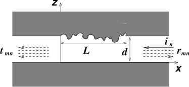
Figure 1: Illustration of the scattering geometry of the surface-disordered waveguide.

The scattering geometry is depicted in Fig. 1. We seek for solutions to the scalar Helmholtz equation in the form (outside the region $0\leq x\leq L$):

$$\Psi_{n}\left(x,\mathbf{r}\right)={\displaystyle\sum_{m}k^{-1/2}_{m}\chi_{m}\left(\mathbf{r}\right)e^{-ik_{m}x}t_{mn},}\quad x<0,$$ (1a)

$$\Psi_{n}\left(x,\mathbf{r}\right)={\displaystyle\Psi^{0}_{n}\left(x,\mathbf{r}\right)}\hskip 113.81102pt$$

$${\displaystyle+\sum_{m}k^{-1/2}_{m}\chi_{m}\left(\mathbf{r}\right)e^{ik_{m}x}r_{mn},}\quad x>L,$$ (1b)

with

$$\Psi^{0}_{n}\left(x,\mathbf{r}\right)=k^{-1/2}_{n}\chi_{n}(\mathbf{r})e^{-ik_{n}x}.$$ (1c)

The indexes “$m,n$” correspond to the outgoing and incoming modes, respectively. $\chi_{n}\left(\mathbf{r}\right)$ are the eigenfunctions of the transverse wave equation, characterized by transverse momentum $\kappa_{n}$, so that the longitudinal wavevector component $k_{n}$ (along the propagation direction) is

$$k_{n}=\left[(\omega/c)^{2}-\kappa_{n}^{2}\right]^{1/2},$$ (2)

with $\omega$ being the wave frequency.

We consider the Dirichlet boundary condition on a slightly perturbed waveguide surface, $\zeta$ denoting the random perturbation, and expand it about the unperturbed surface $\mathbf{R}=\mathbf{R_{s}}$, which is translationally invariant along the $x$-axis [$\mathbf{R}=\left(x,\mathbf{r}\right)$], so that:

$$\Psi\left(\mathbf{R}=\mathbf{R_{s}}\right)=0,\text{ for }x<0\text{ and }x>L,\hskip 36.135pt$$ (3a)

$${\displaystyle=-\mbox{\boldmath$\zeta$}\left(\mathbf{R}\right)\cdot\frac{\partial\Psi\left(\mathbf{R}\right)}{\partial\mathbf{R}},}\text{ for }0\leq x\leq L.$$ (3b)

Alternatively, the latter boundary condition can be associated to a waveguide surface with a random admittance.

It can be shown that the matrices of reflection and transmission coefficients satisfy the following differential equations prb99 :

$$\frac{d\widehat{r}}{dL}=\frac{i}{2}\left(e^{-i\widehat{k}L}+\widehat{r}e^{i\widehat{k}L}\right)\widehat{v}\left(e^{-i\widehat{k}L}+e^{i\widehat{k}L}\widehat{r}\right),$$ (4a)

$$\frac{d\widehat{t}}{dL}=\frac{i}{2}\widehat{t}e^{i\widehat{k}L}\widehat{v}\left(e^{-i\widehat{k}L}+e^{i\widehat{k}L}\widehat{r}\right),$$ (4b)

with $$\widehat{k}=diag\left(k_{n}\right)$$ and

$$v_{mn}=\oint ds\,\phi_{m}\left(s\right)\zeta\left(L,s\right)\phi_{n}\left(s\right),$$

$$\phi_{n}\left(s\right)=k^{-1/2}_{n}\mathbf{n}(\mathbf{r_{s}})\cdot\left[\frac{\partial\chi_{n}\left(\mathbf{r}\right)}{\partial\mathbf{r}}\right]_{\mathbf{r}=\mathbf{r_{s}}};$$

it has been assumed that $\zeta$$=\zeta\mathbf{n}$. The explicit form of the differential $ds$ over the cross section (oriented) surface element $d\mathbf{s}=\mathbf{n}ds$ depends on the geometry under consideration. The reflection and transmission intensities are defined by:

$$R_{mn}=\left|r_{mn}\right|^{2},T_{mn}=\left|t_{mn}\right|^{2},$$ (5)

which yield the intensity coupled into the $mth$ outgoing channel in reflection and transmission, respectively, for a given $nth$ incoming channel.

II.2 Field distribution inside the disordered region

By invoking Green’s theorem, the expression for the field inside the waveguide ($0\leq x\leq L$) can be written as:

$$\Psi_{n}\left(x,\mathbf{r}\right)=\Psi_{n}^{0}\left(x,\mathbf{r}\right)$$

$$+\int\limits_{0}^{L}dx^{\prime}\oint ds^{\prime}\Psi_{n}\left(x^{\prime},\mathbf{r_{s}^{\prime}}\right)\frac{\partial G_{0}\left(x^{\prime},x;\mathbf{r_{s}^{\prime}},\mathbf{r}\right)}{\partial n^{\prime}},$$ (6)

where $\Psi_{n}^{0}=k_{n}^{-1/2}\chi_{n}(\mathbf{r})e^{-ik_{n}x}$. Substituting the Green’s function

$$G_{0}\left(x,\mathbf{r};x^{\prime}\mathbf{r^{\prime}}\right)=\sum_{m=1}^{N}(2ik_{m})^{-1}\chi_{m}\left(\mathbf{r}\right)\chi_{m}\left(\mathbf{r^{\prime}}\right)e^{ik_{m}\left|x-x^{\prime}\right|}$$ (7)

into Eq. (6), we end up with the following expression for the scattered field inside:

$$\Psi_{n}^{sc}\left(x,\mathbf{r}\right)=\Psi_{n}\left(x,\mathbf{r}\right)-\Psi_{n}^{0}\left(x,\mathbf{r}\right)\hskip 72.26999pt$$

$$=\int\limits_{0}^{L}dx^{\prime}\oint ds^{\prime}\Psi_{n}\left(x^{\prime},\mathbf{r_{s}^{\prime}}\right)\hskip 57.81621pt$$

$$\times\sum_{m=1}^{N}(2ik_{m})^{-1}\chi_{m}(\mathbf{r})\frac{\partial\chi_{m}(\mathbf{r_{s}^{\prime}})}{\partial n^{\prime}}e^{ik_{m}|x-x^{\prime}|},$$ (8)

where $\Psi_{n}^{0}=k_{n}^{-1/2}\chi_{n}(\mathbf{r})e^{-ik_{n}x}$. Rearranging the integrand, and handling the phase factor $e^{ik_{m}|x-x^{\prime}|}$ appropriately by splitting the integral along the waveguide $\int\limits_{0}^{L}=\int\limits_{0}^{x}+\int\limits_{x}^{L}$, one obtains:

$$\Psi_{n}^{sc}\left(x,\mathbf{r}\right)=\sum_{m=1}^{N}(2ik_{m})^{-1/2}\chi_{m}(\mathbf{r})\hskip 79.49744pt$$

$$\times\left\{\int\limits_{0}^{x}dx^{\prime}e^{ik_{m}(x-x^{\prime})}\oint ds^{\prime}\Psi_{n}\left(x^{\prime},\mathbf{r_{s}^{\prime}}\right)\frac{\partial\chi_{m}(\mathbf{r_{s}^{\prime}})}{\partial n^{\prime}}\right.$$

$$\left.+\int\limits_{x}^{L}dx^{\prime}e^{-ik_{m}(x-x^{\prime})}\oint ds^{\prime}\Psi_{n}\left(x^{\prime},\mathbf{r_{s}^{\prime}}\right)\frac{\partial\chi_{m}(\mathbf{r_{s}^{\prime}})}{\partial n^{\prime}}\right\}.$$ (9)

Factoring out the phase factors defining waves propagating right and left, and splitting again the integral of the second term, we get

$$\Psi_{n}^{sc}\left(x,\mathbf{r}\right)=\sum_{m=1}^{N}\frac{\chi_{m}(\mathbf{r})}{k_{m}^{1/2}}\left\{\frac{e^{ik_{m}x}}{2ik_{m}^{1/2}}\right.\hskip 86.72377pt$$

$$\times\int\limits_{0}^{x}dx^{\prime}\oint ds^{\prime}\Psi_{n}\left(x^{\prime},\mathbf{r_{s}^{\prime}}\right)\frac{\partial\chi_{m}(\mathbf{r_{s}^{\prime}})}{\partial n^{\prime}}e^{-ik_{m}x^{\prime}}+\frac{e^{-ik_{m}x}}{2ik_{m}^{1/2}}$$

$$\left.\left(\int\limits_{0}^{L}dx^{\prime}-\int\limits_{0}^{x}dx^{\prime}\right)\oint ds^{\prime}\Psi_{n}\left(x^{\prime},\mathbf{r_{s}^{\prime}}\right)\frac{\partial\chi_{m}(\mathbf{r_{s}^{\prime}})}{\partial n^{\prime}}e^{ik_{m}x^{\prime}}\right\}.$$ (10)

At this point, we define the local amplitudes of the scattered waves propagating along the $x$ axis in positive and negative directions, respectively, $\rho(x)$ and $\tau(x)$:

$$\rho_{mn}^{L}(x)=(2ik_{m}^{1/2})^{-1}\hskip 108.405pt$$

$$\times\int\limits_{0}^{x}dx^{\prime}\oint ds^{\prime}\Psi_{n}\left(x^{\prime},\mathbf{r_{s}^{\prime}}\right)\frac{\partial\chi_{m}(\mathbf{r_{s}^{\prime}})}{\partial n^{\prime}}e^{-ik_{m}x^{\prime}},$$ (11a)

$$\tau_{mn}^{L}(x)=t_{mn}(L)-\delta_{mn}-(2ik_{m}^{1/2})^{-1}\hskip 36.135pt$$

$$\times\int\limits_{0}^{x}dx^{\prime}\oint ds^{\prime}\Psi_{n}\left(x^{\prime},\mathbf{r_{s}^{\prime}}\right)\frac{\partial\chi_{m}(\mathbf{r_{s}^{\prime}})}{\partial n^{\prime}}e^{ik_{m}x^{\prime}},$$ (11b)

so that

$$\Psi^{sc}_{n}\left({\bf R}\right)=\sum_{m=1}^{N}k_{m}^{-1/2}\chi_{n}({\bf r})\hskip 86.72377pt$$

$$\times\{\rho^{L}_{mn}(x)e^{ik_{m}x}+\tau^{L}_{mn}(x)e^{-ik_{m}x}\}.$$ (12)

Then, by differentiating Eqs. (11), and taking into account the boundary condition (3) in the integrands, with the aid of Eq.  (12) again, a set of coupled differential equations for $\rho_{mn}^{L}(x)$ and $\tau_{mn}^{L}(x)$ is derived:

$$\frac{d\widehat{\rho}^{L}}{dx} = \frac{i}{2}e^{-i\widehat{k}x}\widehat{v}\left[e^{-i\widehat{k}x}(\widehat{I}+\widehat{\tau}^{L})+e^{i\widehat{k}x}\widehat{\rho}^{L}\right],$$ (13a)

$$\frac{d\widehat{\tau}^{L}}{dx} = -\frac{i}{2}e^{i\widehat{k}x}\widehat{v}\left[e^{-i\widehat{k}x}(\widehat{I}+\widehat{\tau}^{L})+e^{i\widehat{k}x}\widehat{\rho}^{L}\right].$$ (13b)

The corresponding boundary conditions satisfied by $\rho_{mn}^{L}(x)$ and $\tau_{mn}^{L}(x)$ at the end points of the waveguide are:

$$\rho_{mn}^{L}(x = 0)=0,\tau_{mn}^{L}(x=0)=t_{mn}(L)-\delta_{mn};$$ (14)

$$\rho_{mn}^{L}(x = L)=r_{mn}(L),\tau_{mn}^{L}(x=L)=0.$$ (15)

II.3 Numerical calculations

We have chosen for the numerical simulations the same geometry as in Ref. prb99, : two parallel, perfectly reflecting planes at $z=0$ and $z=d$ with random deviations $z=\zeta\left(x\right)$ given by a 1D stochastic process with Gaussian statistics with zero mean and a Gaussian surface power spectrum

$$g(Q)=\delta^{2}\pi^{\frac{1}{2}}a\exp\left(-(Qa)^{2}/4\right),$$ (16)

where $\delta$ is the RMS height and $a$ is the transverse correlation length. The corresponding transverse eigenfunctions are thus given by

$$\chi_{n}\left(z\right)=(2/d)^{1/2}\sin\left(\kappa_{n}z\right),\;\kappa_{n}=\pi n/d,$$ (17)

and the impurity matrix (II.1) by

$$v_{mn}\left(L\right)=\frac{2}{d}\frac{\kappa_{n}\kappa_{m}}{(k_{n}k_{m})^{1/2}}\zeta\left(L\right).$$ (18)

In order to model 1D wave propagation in our calculations, the waveguide supports only one mode, its thickness $d$ being such that $\bar{\omega}\equiv\omega d/(2\pi c)\approx 0.75$. Consequently, all subscripts referring to mode indexes are suppressed hereafter.

The linear differential equations for the reflection and transmission amplitudes (4) are solved numerically by means of the Runge-Kutta method; this is done for a given realization $\zeta(x)$ from $L=0$ up to a maximum length $L=L_{max}$ (cf. Ref. prb99, ). Then, for a fixed length of the disordered segment $L$, the same standard numerical techniques are employed for the system of first-order differential Eqs. (13) in order to obtain the local reflection and transmission amplitudes, with the help of the boundary conditions (15) involving the reflection and transmission amplitudes [$r(L),t(L)$], previously obtained. Finally, the field intensity is calculated from the incident and scattered fields inside [Eqs. (1c) and (12)]:

$$I(x)=\mid\Psi(x,d/2)/\Psi^{0}(x,d/2)\mid^{2}.$$ (19)

II.4 Analytical approach: Rapid phase averaging

To calculate analytically the average intensity, $\left\langle I(x)\right\rangle$, inside a one-dimensional disordered system we introduce the function

$$R(x)=\frac{\rho(x)}{\tau(x)+1}\exp(2ikx),$$ (20)

that satisfies the nonlinear equation

$$i\frac{dR(x)}{dx}=-2kR(x)+\frac{V(x)}{2k}[1+R(x)]^{2},\text{ \ }$$ (21)

where $k$ is the longitudinal wave number of the propagating mode ($k=\left[(\omega/c)^{2}-\left(\pi/d\right)^{2}\right]^{1/2})$. The random scattering potential, $V(x)$, in the case under consideration, i.e. in a single-mode waveguide with a randomly rough surface, has the form:

$$V(x)=-\frac{2\pi}{d^{3}}\zeta\left(x\right).$$ (22)

Then the intensity can be expressed as klbook

$$I(x)=I_{0}\left[1-\left|R(x)\right|^{2}\right]\frac{1+\left|R(x)\right|^{2}+2\Re(R(x))}{1-\left|R(x)\right|^{2}}.$$ (23)

Obviously, $R(L)=r(L)\exp(2ikL)$ where $r(L)$ is the total reflection coefficient of a single-mode waveguide defined by Eq. (4a). It is convenient, following Ref. klbook, , to introduce two functions, $u(x)$ and $\varphi(x)$, so that

$$R(x)=\sqrt{\frac{u(x)-1}{u(x)+1}}\exp\left[i\varphi(x)\right].$$ (24)

Substitution of Eq. (24) into Eq. (23) yields

$$I(x)=\frac{2I_{0}}{u(L)+1}\left[u(x)+\sqrt{u^{2}(x)-1}\cos\varphi(x)\right].$$ (25)

If the scattering is weak enough, so that $l_{scat}\gg\lambda$, the random phase, $\varphi(x)$, is uniformly distributed over $[0,2\pi]$; We have verified this assumption through numerical calculations of the probability density function of $\varphi(x)$ (not shown here), which indeed yield a uniform distribution in all cases studied below. Obviously, to get rid of the rapid (on the scale of order of $\lambda)$ oscillations of the phase one has to integrate (average) Eq. (25) over an interval $\pounds$ that satisfies the inequality $\lambda\ll\pounds\ll l_{scat}.$ This rapid phase averaging (RPA) yields

$$I(x)=\frac{2I_{0}u(x)}{u(L)+1}.$$ (26)

The two-point probability distribution function, $p_{2}(u_{L},L;u_{x},x)$, necessary for the ensemble averaging of the intensity $I(x)$, Eq. (26), can be also calculated under the assumptions that $l_{scat}\gg\lambda$ and that the scattering potential is a $\delta$-correlated Gaussian random process such that

$$\langle\delta V(x)\delta V(x^{{}^{\prime}})\rangle=D\delta(x-x^{{}^{\prime}}).$$ (27)

Then, the smoothed (RPA) mean intensity distribution inside a one-dimensional random system can be presented in the form klbook

$$\left\langle I(x)\right\rangle=\pi\exp[D(x-L/4)]\int_{0}^{\infty}d\mu\frac{\sinh\mu\pi}{\cosh^{2}\mu\pi}$$

$$\times\exp(-\mu^{2}DL)\left(\cos 2\mu Dx+\frac{\sin 2\mu Dx}{2\mu}\right).$$ (28)

In what follows, comparisons with the numerical calculations will be made on the basis of the average (macroscopic) properties, regardless of the (microscopic) details of the disorder. Namely, the localization length $\xi$, defined from $\langle\log T\rangle\sim-L/\xi$, will be used as matching parameter, which in this RPA approach is given by $\xi=D^{-1}$.

III SINGLE REALIZATIONS: RESONANCES

First, we identify the roughness and waveguide parameters that lead to the onset of Anderson localization. This is done in Fig. 2 by plotting the length dependence of $\langle\log T\rangle$ at frequency $\bar{\omega}=0.75$ (single mode) for several RMS heights $\delta$ and fixed correlation length $a/d=0.2$. The resulting linear decay is the fingerprint of Anderson localization, the decay rate yielding the localization length. The fitted values of $\xi$ for each $\delta$ are included in Fig. 2.

With the aid of the latter results, we choose a set of parameters that ensure the 1D Anderson localization regime: $a/d=0.2$, $\delta/d=0.05$, and $L=1500d\approx 5.5\xi$. We then calculate the frequency dependence (in a narrow frequency range) of the transmission coefficient $T(\omega)$ for a given realization, as shown in Fig. 3(a). Extremely large fluctuations are observed with narrow spikes appearing over a fairly negligible background. The latter background yields the expected response at typical (high probability) frequencies, since $\langle\log T(\bar{\omega}=0.75)\rangle\sim-5.2$ and $\langle T(\bar{\omega}=0.75)\rangle\sim 0.062$. The low-probability peaks in Fig. 3(a) correspond to narrow resonances or quasi-transparent frequencies at which the transmission coefficient can be even 1.

The transmission in the vicinity of one such transparent frequency ($\bar{\omega}_{0}=0.75069$) is presented in detail in Fig. 3(b). Note the frequency scale, revealing how narrow the resonance is. By fitting the numerical result to a Lorentzian [also shown in Fig. 3(b)], we obtain the half-width at half-maximum $\Gamma/\omega_{0}\approx 2.4\times 10^{-6}$. Resonances behave like high-finesse cavity modes with large associated $Q$-factors ($\sim 3\times 10^{5}$), which may lead to practical applications as in random lasing cao ; natu ; lag01 .

The field intensities inside the waveguide for frequencies at the resonance, mid-resonance, and out-of-resonance [$\bar{\omega}=0.75069,0.7506875$, and 0.7506, respectively, in Fig. 3(b)] are shown in Fig.  4, where the envelope and average of $I(x)$ over rapid oscillations (period $\sim\pi/k$) are plotted. The incident mode impinges on the disordered segment at $x=L$ propagating from right (positive $x$ axis) to left (negative $x$ axis). At resonance [see Fig. 4(a)], high intensity concentration takes place over a region around the center of the disordered segment of the waveguide ($I\sim 200$ with a peak of $I\sim 400$), its particular shape being a characteristic feature of the given resonance. The field intensity at the end points (not discernible in the figure) is $I(x=0,L)=1$, as expected ($T=1,R=0$). At mid-resonance [see Fig. 4(b)], the field intensity distribution maintains its shape, but the overall height is decreased by nearly a factor of 2. The reflected and transmitted coefficients are retrieved at the end points: $I(x=L)=\mid 1+r\exp(ikL)\mid^{2}$ (envelope $\approx 2.25$ and mean $\approx 1.5$) and $I(x=0)=T\approx 0.25$.

In contrast, an absolutely different behavior has been observed away from resonance, i.e. at typical (non-transparent) frequencies (or realizations), as seen in Fig. 4(c). The field energy is not localized, but decays from its initial value $I(x=L)$ (envelope $\approx 4$ and mean $\approx 2$) to the exponentially small value $I(x=0)=T\sim\exp(-L/\xi)$.

IV TOTAL, TYPICAL AND RESONANT AVERAGE FIELDS

We now turn to the analysis of the ensemble average of the field intensity $\langle I(x)\rangle$ along the disordered region. Numerical simulation calculations are carried out for fixed $\bar{\omega}=0.75$, $L$, and statistical parameters of the roughness. Averages have been done over $N=10^{5}$ realizations, separating typical and resonant realizations according to a threshold value of the mean transmission coefficient $T_{c}$.

Figure 5(a) shows $\langle I(x)\rangle$ for $a/d=0.2$, $\delta/d=0.05$, and various values of the disordered segment length $L/d=1200,1500,2250,3000$. (Recall that the incident mode impinges on the disordered segment from the right end, $x=L$, which we have shifted to the origin for the sake of clarity.) In all cases, the mean intensity decays monotonically towards the exit of the disordered waveguide, the decay rate being smaller the longer is the waveguide (provided that $L/\xi\gg 1$). The contribution from resonances to the mean intensity, $\langle I(x)\rangle_{reso}$, yielding transmission coefficients larger than $T_{c}=0.4$, is shown in Fig. 5(b). Broad distributions are found with large maximum field intensities lying near the center of the disordered waveguide. The contribution from typical realizations ($>90\%$), $\langle I(x)\rangle_{typ}$ is plotted in Fig. 5(c); a qualitative behavior similar to that of the total mean intensity is observed, except for a faster decay rate.

In order to improve our understanding of the physics underlying the formation of the field intensity patterns, we have replotted $\langle I(x)\rangle$ by rescaling the $x$-dependence in units of the disordered segment length $L$, $\bar{x}=(x-L/2)/L$. In addition to that, calculations have been done for different roughness parameters $\delta/d=0.05,0.08$ and 0.1 (fixed $a/d=0.2$), by choosing $L$ in such a way that the ratio $L/\xi$ remains fixed (the corresponding values of the localization length $\xi$ are given in Fig. 2). The resulting $\langle I(x)\rangle$ are presented in Fig. 6: The RPA quasi-analytical results obtained from Eq. (28) are also included.

Several conclusions can be drawn from the latter results. First, $\langle I(\bar{x})\rangle$ exhibits in all cases a universal behavior, depending only on the ratio $L/\xi$ regardless of the microscopic details of the 1D disorder. Actually, as shown in the inset in Fig. 2, we have observed that universality can be pushed further, so that $\langle I(\tilde{x})\rangle$ [with $\tilde{x}=(x-L/2)/(L\xi)^{1/2}$] is a unique function. Second, for moderate and even large $L/\xi$, the RPA expression predicts very accurately the mean field distribution obtained numerically; a monotonic decay from $\langle I(\bar{x}=0.5)\rangle=1+\langle R(L)\rangle$ at the incoming end to $\langle I(\bar{x}=-0.5)\rangle=\langle T(L)\rangle$, crossing the value $\langle I\rangle=1$ through the middle of the disordered segment $\bar{x}=0$, and being steeper the larger is $L/\xi$. Third, deep into the 1D Anderson localization regime, $L/\xi\geq 11$ in Fig. 6, the numerical results reveal a departure from the RPA predictions, as evidenced by the shift of the $\langle I\rangle=1$ crossing towards the incoming end. We have investigated the physical origin of this discrepancy by enforcing in the numerical calculations some of the assumptions made in the RPA approach. First, uncorrelated disorder has been used in the numerical calculations, with similar results to those for the Gaussian correlation. Rapid phase averaging has also been carried out at each realization prior to ensemble averaging, yielding no significant differences. Thus neither finite correlation nor RPA can give rise to the observed discrepancy.

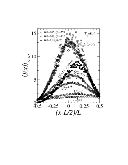
Figure 7: Same as in Fig. 6 but for the contribution from resonant realizations with $T_{c}=0.4$ (hollow symbols, $L/\xi=1,2,4.4,5.5,8.2$) and $T_{c}=0.01$ (filled symbols, $L/\xi=11$).

At this point, it is important to emphasize that plotted in Fig. 6 is the ensemble average of the intensity, which is a non-self-averaging (strongly fluctuating) quantity. To gain insight into the behavior of the field intensity pattern at different individual realizations, we have separated typical and resonant realizations according to a threshold value, $T_{c}$, of the mean transmission coefficient. The contribution from resonances to the mean intensity, $\langle I(x)\rangle_{reso}$, and (rescaled) $\langle I(\bar{x})\rangle_{reso}$, yielding transmission coefficients larger than $T_{c}=0.4$, is shown in Figs. 5(b) and 7. One can see that the contribution from resonances also exhibits universal behavior in the form of a broad distribution with a relatively large maxima within the disordered segment, being determined not only by the ratio $L/\xi$ (as in the case of the total average), but also by the the cutoff parameter $T_{c}$. Actually, from the comparison of the curves for $\langle I(\bar{x})\rangle_{reso}$ with different $T_{c}$ in Fig. 7, it follows that $T_{c}$ fixes the position of the maximum intensity, whereas the ratio $L/\xi$ sets the precise value of the maxima. For fixed $T_{c}$, the maximum intensity is higher for larger $L/\xi$; namely, stronger resonances are needed for longer disorder in order to couple the same amount of energy through the system (or similarly, to tunnel through a wider barrier). Relaxing the definition of resonance (lowering $T_{c}$) for fixed ratio $L/\xi$ (see Fig. 7), leads to asymmetrical $\langle I(\bar{x})\rangle_{reso}$ distributions with maxima shifted from the center to the incoming end of the disorder segment.

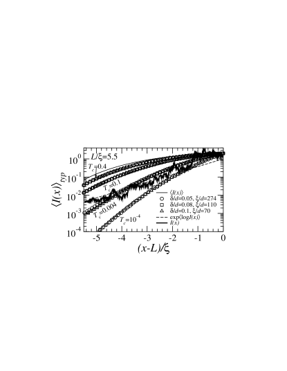
Figure 8: Spatial distributions of the contribution to the average field intensity (log scale) from typical realizations with $a/d=0.2$, $\delta/d=$0.05 (circles), 0.08 (squares), and 0.1 (triangles), and fixed disordered length $L/\xi=5.5$, for $T_{c}=10^{-4}$, 0.004, 0.1, 0.4, and 1 (the latter equivalent to $\langle I(x)\rangle$, thin solid curve). Also included are: $\exp\langle\log I(x)\rangle$ (dashed curve) and $I(x)$ (spatially averaged in a log scale) for a single, typical realization (thick solid curve).

The contribution to the average intensity from typical realizations ($>90\%$), $\langle I(x)\rangle_{typ}$, plotted in Fig. 5(c), also depends universally on $L/\xi$ and $T_{c}$ (not shown here), and shows a qualitative behavior similar to $\langle I(x)\rangle$, with a faster decay, as expected. Interestingly, neither $\langle I(x)\rangle$ nor $\langle I(x)\rangle_{typ}$ decay exponentially, but rather manifest a $s$-like dependence, as mentioned above. This means that, no matter how long the realization is [i.e., how small is $\exp(-L/\xi)$], a lengthening of the system (increase of $L$ with the localization length kept fixed) leads, surprisingly enough, to essential changes in the energy distribution inside. Namely, provided that the strength of the disorder is fixed, the longer a randomly disordered sample is, the slower is the decay of the intensity [both $\langle I(x)\rangle$ and $\langle I(x)\rangle_{typ}$] from the incoming end deep into the sample [this is neatly observed in Figs. 5(a) and  5(c)]. In other words, the ”penetration depth” of both $\langle I\rangle$ and $\langle I\rangle_{typ}$ into a 1D random system is independent of the strength of scattering. This effect is, however, dependent on the value $T_{c}$ in the definition of $\langle I\rangle_{typ}$, as illustrated in Fig. 8: with the cutoff decreasing, the slowly decaying part of $\langle I(x)\rangle_{typ}$ near the incoming end ($x=L$) diminishes, the distribution thus decaying more abruptly. Obviously, the longer a realization is, the smaller $T_{c}$ is necessary for the transition to take place. Interestingly, the intensity for a single typical realization for which $T\sim\langle T\rangle$ appears to decay approximately exponentially $I\sim\exp(-x/\xi)$, as seen in Fig. 8 (its oscillations are smoothed spatially on a log scale). This is in accordance with the behavior of the average logarithm of the intensity, which fluctuates less strongly than the intensity itself and fits very accurately $\langle\log I(x)\rangle\simeq-|x-L|/\xi$ (see Fig. 8), revealing its self-averaging nature.

Finally, we have calculated higher-order moments of the mean intensity $\langle I^{n}(\bar{x})\rangle$. In Fig. 9, the numerical results are shown in the case $n=2,4$ for some of the disordered waveguides considered above. The most remarkable feature is the broad, resonant-like shape, revealing the increasing (for higher $n$) influence of (low-probability) resonances, with huge field intensities.

V CONCLUDING REMARKS

To summarize, we have developed a formalism to calculate the field inside surface-disordered waveguides, similar to that of the invariant embedding equations for the reflection and transmission coefficients. By applying it to 2D single-mode waveguides with planar walls and Gaussian-correlated surface roughness, we have investigated the occurrence of resonances in the 1D Anderson localization regime, with emphasis on the resulting field intensity distribution both for given realizations and ensemble averages.

We have examined the frequency dependence of the transmission coefficient $T(\omega)$ for different realizations; it exhibits well-defined resonance-type behavior inherent to the localization regime. This enables us to separate typical realizations, characterized by very low (as expected from the average $\langle\log T\rangle\sim-L/\xi$) values of $T$ and a monotonically decaying intensity, from resonances with transmission coefficients close to one and extremely high intensity maxima (localization) in a region around the center of the system.

Numerical simulation calculations for the mean field intensity $\langle I(x)\rangle$ along the disordered segment of the waveguide reveal a universal behavior completely determined by the ratio $L/\xi$: A smooth decay from the initial value of $\langle I\rangle\sim 1+\langle R(L)\rangle$ at the incoming end, to the outgoing mean transmitted field intensity $\langle I\rangle\sim\langle T(L)\rangle$, crossing the value $\langle I\rangle\sim 1$ at/near the center of the disordered segment. For moderately strong disorder $L/\xi\overset{>}{\sim}1$, the quasi-analytical (RPA) prediction (28) fully agrees with the numerical calculations. However, for strong disorder $L/\xi\gg 1$, the numerical results exhibit, unlike the RPA result, a shift of the mid-point ($\langle I\rangle\sim 1$) towards the incoming edge. The contribution to $\langle I(x)\rangle$ from resonant realizations (those yielding anomalously large transmission above a threshold value $T_{c}$) manifests also universality characterized by the parameters $L/\xi$ and $T_{c}$: Its shape is a broad distribution whose maximum value, which is larger for stronger disorder, shifts from the center towards the incoming edge with decreasing $T_{c}$. On the other hand, we have found that the contribution from such low-probability resonances become more dramatic in higher-order moments of the total intensity distribution.

The contribution from typical realizations to the total average, $\langle I(x)\rangle_{typ}$, depends on the cutoff value $T_{c}$. For $T_{c}$ not too small, $\langle I(x)\rangle_{typ}$ (as well as $\langle I(x)\rangle$) inside a 1D random system is slightly dependent on the strength of the scattering, and increases with the increase of the total length, $L$, of the system. With decreasing threshold value $T_{c}$, the penetration depth ceases to depend on $L$ and $\langle I(x)\rangle_{typ}$ decays more rapidly. In this regard, evidence of the self-averaging nature of $\log I(x)/x$ is given by the behavior of $\log I(x)$ for single, typical realizations, and also by the result that $\langle\log I(x)\rangle\simeq-|x-L|/\xi$.

Figure 2: Average logarithm of the transmission coefficient over $N=10^{5}$ realizations as a function of the disorder length $L$ for surface roughness parameters $a/d=0.2$ and $\delta/d=0.0125,0.025,0.04,0.05,0.08,0.1$. The localization lengths $\xi$ resulting from fits to linear decays are shown.

Figure 3: (a) Spectral dependence of the transmission coefficient for a given disorder realization with $a/d=0.2$, $\delta/d=0.05$, and $L/d=1500$ in a narrow frequency range showing several resonant frequencies. (b) A single resonance is zoomed in and fitted to a Lorentzian (dashed curve, indistinguishable from the numerical result.

Figure 4: Field intensity along the disorder realization used in Fig. 3(b) (with $a/d=0.2$, $\delta/d=0.05$, and $L/d=1500$) at (a) $\bar{\omega}\equiv\omega d/(2\pi c)=$0.75069 (resonance), (b) $\bar{\omega}=$0.7506875 (mid-resonance), and (c) $\bar{\omega}=$0.7506 (out of resonance, typical). To suppress rapid spatial oscillations, the envelopes (upper curves) and spatial averages (lower curves) are shown. The incident wave is coming from the right end.

Figure 5: (a) Spatial distributions of average field intensity ($N=10^{5}$ realizations) for $a/d=0.2$, $\delta/d=0.05$, and disorder lengths: $L/d=$550 (curves A), 1500 (curves B), 2250 (curves C), and 3000 (curves D). All curves have been shifted to make coincide the incoming ends at $x=0$. The contributions from resonant realizations (with $T\geq T_{c}=0.1$) and the remaining typical realizations are shown in (b) and (c), respectively.

Figure 6: Spatial distributions of average field intensity ($N=10^{5}$ realizations) as a function of renormalized position $\bar{x}\equiv(x-L/2)/L$ for $a/d=0.2$ and $\delta/d=$0.05 (circles), 0.08 (squares), and 0.1 (triangles). In each case, several disordered lengths are considered according to $L/\xi=0.5,1,2,4.4,8.2,11$. Solid curves represent the quasi-analytical, RPA results. Inset: the RPA results only as a function of $\tilde{x}\equiv(x-L/2)/(L\xi)^{1/2}$.

Figure 9: Same as in Fig. 6 but for the 4th (a) and 2nd (b) moments of the field intensity, and $L/\xi=2,4.4,8.2$.

- (1) U. Frisch, C. Froeschle, J.-P. Scheidecker, and P.-L. Sulem, Phys. Rev. A8, 1416 (1973).
- (2) G. Papanicolaou, J. Appl. Math. 21, 13 (1971); W. Kohler, G. Papanicolaou, J. Math. Phys. 14, 1753 (1973); W. Kohler, G. Papanicolaou, J. Math. Phys. 15, 2186 (1974); J. Keller, G. Papanicolaou, J. Weilenmann, J. Appl. Math. 32, 583 (1978).
- (3) M. Ya. Azbel, Phys. Rev. B22, 4045 (1980); M. Ya. Azbel, Phys. Rev. Lett. 47, 1015 (1981); M. Ya. Azbel, P. Soven, Phys. Rev. Lett. 49 , 751 (1982); M. Ya. Azbel, Phys. Rev. B28, 4106 (1983); M. Ya. Azbel, P. Soven, Phys. Rev. B27, 831 (1983); M. Ya. Azbel, Phys. Rev. B27, 3901 (1983); E. Cota, J. V. Jose, and M. Ya. Azbel, Phys. Rev. B32, 6157 (1985)
- (4) V. Kliatzkin, Stochastic Equations and Waves in Random Media (Nauka, Moscow, 1980), in Russian.
- (5) I. M. Lifshits, S. A. Gredeskul, and L. A. Pastur, Introduction to the Theory of Disordered Systems (Wiley, New York, 1988), Chap. 7.
- (6) Scattering and Localization of Classical Waves in Random Media, edited by P. Sheng (World Scientific, Singapore, 1990).
- (7) V. Freilikher and S. Gredeskul, Progress in Optics 30, 137 (1992).
- (8) V. S. Letokhov, Sov. Phys. JETP 26, 835 (1968).
- (9) H. Cao, Y. G. Zhao, S. T. Ho, E. W. Seelig, Q. H. Wang, and R. P. H. Chang, Phys. Rev. Lett. 82, 2278 (1999); H. Cao, Y. Ling, J. Y. Xu, C. Q. Cao, and P. Kumar, Phys. Rev. Lett. 86, 4524 (2001).
- (10) D. S. Wiersma, Nature 406, 132 (2000); D. S. Wiersma, S. Cavalieri, Nature 414, 708 (2001).
- (11) G. van Soest, F. J. Poelwijk, R. Sprik, and Ad Lagendijk, Phys. Rev. Lett. 86, 1522 (2001).
- (12) J. A. Sánchez-Gil, V. Freilikher, I. V. Yurkevich, and A. A. Maradudin, Phys. Rev. Lett. 80, 948 (1998).
- (13) A. García-Martín, J. A. Torres, J. J. Sáenz, and M. Nieto-Vesperinas, Phys. Rev. Lett. 80, 4165 (1998); A. García-Martín, T. López-Ciudad, J. J. Sáenz, and M. Nieto-Vesperinas, Phys. Rev. Lett. 81, 329 (1998).
- (14) J. A. Sánchez-Gil, V. Freilikher, A. A. Maradudin, and I. Yurkevich, Phys. Rev. B59, 5915 (1999).
- (15) A. García-Martín, J. J. Sáenz, and M. M. Nieto-Vesperinas, Phys. Rev. Lett. 84, 3578 (2000).
- (16) A. García-Martín and J. J. Sáenz, Phys. Rev. Lett. 87, 116603 (2001).
- (17) A. García-Martín, F. Scheffold, M. Nieto-Vesperinas, and J. J. Sáenz, Phys. Rev. Lett. 88, 143901 (2002).
- (18) F. M. Izrailev and N. M. Makarov, Opt. Lett. 26, 1604 (2002).
- (19) N. Makarov and I. Yurkevich, Zh. Éksp. Teor. Fiz. 96, 1106 (1989) [Sov. Phys. JETP 69, 628 (1989)]; A. Krokhin, N. Makarov, V. Yampolskii, and I. Yurkevich, Physica B 165&166, 855 (1990); V. Freilikher, M. Pustilnik, and I. Yurkevich, Phys. Rev. Lett. 73, 810 (1994).