Analytical and Numerical Treatment of the Mott–Hubbard Insulator in Infinite Dimensions

Abstract

We calculate the density of states in the half-filled Hubbard model on a Bethe lattice with infinite connectivity. Based on our analytical results to second order in $t/U$, we propose a new ‘Fixed-Energy Exact Diagonalization’ scheme for the numerical study of the Dynamical Mean-Field Theory. Corroborated by results from the Random Dispersion Approximation, we find that the gap opens at $U_{\rm c}=4.43\pm 0.05$. Moreover, the density of states near the gap increases algebraically as a function of frequency with an exponent $\alpha=1/2$ in the insulating phase. We critically examine other analytical and numerical approaches and specify their merits and limitations when applied to the Mott–Hubbard insulator.

1 Introduction

The Mott–Hubbard metal-insulator transition is a fascinating but very difficult problem in condensed matter theory Mottbook ; Gebhardbook ; RMP ; Imada . One hopes that the basic mechanism can be understood with the help of conceptually simple models such as the Hubbard Hamiltonian. This model describes spin-1/2 electrons which move on a lattice (band-width $W=4t$) and interact locally with strength $U$. For small interactions, $U\ll W$, the model describes a metal with a finite density of states at the Fermi energy. For large interactions, $U\gg W$, and when there is on average one electron per lattice site (half band-filling), the model describes an insulator because it takes an energy of the order of $\Delta(U\gg W)\approx U-{\cal O}(W)>0$ to generate a charge excitation, i.e., the single-particle gap $\Delta(U\gg W)$ is finite, irrespective of any symmetry breaking Mottbook ; Gebhardbook .

These basic insights leave much room for speculations on the properties of the transition itself, for example, on the precise value of the critical interaction strength $U_{\rm c}$ at which the gap opens. Because the Mott–Hubbard transition is a zero-temperature quantum phase transition Gebhardbook , it is difficult to access reliably using analytical or numerical techniques; only exact solutions for all interaction strengths can provide conclusive answers. Unfortunately, Hubbard-type models can be solved exactly only in one dimension LiebWu ; GebhardRuckenstein , and several features in one dimension are not generic to three-dimensional systems.

The phase diagram of a model in three dimensions can often be understood from the limit of infinite dimensions. For correlated lattice electrons MV ; MHa , this has led to the formulation of effective single-impurity models whose dynamics must be solved self-consistently (Dynamical Mean-Field Theory, DMFT) RMP ; BrandtMielsch ; Jarrell . An alternative approach, the Random Dispersion Approximation (RDA) Gebhardbook ; RDA , also becomes exact in the limit of infinite dimensions. However, an exact solution of the DMFT is not feasible because single-impurity models with a Hubbard interaction cannot be solved in general.

Using various kinds of approximations, two different scenarios for the Mott–Hubbard transition have been proposed:

Discontinuous Transition.

The gap jumps to a finite value when the density of states at the Fermi energy becomes zero at some critical interaction strength $U_{{\rm c},2}$; the gap is preformed above $U_{{\rm c},1}<U_{{\rm c},2}$, and the co-existing insulating phase is higher in energy than the metallic state.

Continuous Transition.

The gap opens continuously when the density of states at the Fermi energy becomes zero, $U_{{\rm c},1}=U_{{\rm c},2}\equiv U_{\rm c}$.

Various approaches to the Mott–Hubbard transition for lattices with infinite coordination number yield results in favor of one or the other of the conflicting scenarios; for a review, see Refs. Gebhardbook ; RMP . Refs. RDA –Ono give more recent treatments. Insightful physical arguments have helped to sharpen the physical and mathematical implications of the scenario of a preformed gap transition KotliarFisher –Kotliarreply but have not been able to resolve the issue.

All analytical approaches BullaLDMFT –LMA are necessarily approximate in nature, and numerical investigations 7Schwaben –andere of the dynamical mean-field equations involve (i) discretization, (ii) numerical diagonalization, (iii) interpolation, (iv) iteration of the self-consistency cycle, and (v) extrapolation to the thermodynamic limit. The Random Dispersion Approximation RDA requires similar steps in its numerical implementation, apart from step (iv). Therefore, the region of applicability of the available numerical techniques is not a priori clear either.

In order to address this issue, two of us (E.K. and F.G.) have developed a strong-coupling perturbation theory at zero temperature Eva which provides a benchmark test for the available analytical and numerical techniques for the Mott–Hubbard insulator. We assess the quality of the Iterated Perturbation Theory (IPT) and the Local Moment Approach (LMA) as well as three numerical methods for the Hubbard model in infinite dimensions: the Random Dispersion Approximation and two Exact Diagonalization (ED) schemes for the Dynamical Mean-Field Theory. As we shall show, this comparison will provide insight as to the limitations of the various methods and will motivate an improved ED scheme, the ‘Fixed-Energy Exact Diagonalization’ (FE-ED). This scheme successfully reproduces our findings from the $t/U$ expansion even down to the collapse of the Mott–Hubbard insulator.

In this work, after the introduction of some definitions in Sect. 2, we reanalyze our strong-coupling perturbation theory to second order in $t/U$ for the Bethe lattice with infinite connectivity. In Sect. 3 we estimate that the Mott–Hubbard insulator is destroyed at $U_{\rm c}^{\rm sc}/t=4.40\pm 0.09$. In Sect. 4 we set up the Fixed-Energy Exact Diagonalization scheme for the Dynamical Mean-Field Theory. The FE-ED very well reproduces our analytical findings, and confirms our conjecture for the critical interaction strength, $U_{\rm c}^{\rm FE-ED}/t=4.43\pm 0.05$. In Sect. 5 we favorably compare our results with those from the Random Dispersion Approximation (RDA) which provides an independent check on our results from the strong-coupling expansion and the FE-ED. Therefore, we are confident that we accurately describe the Mott–Hubbard insulator for all interaction strengths.

In Sect. 6 we compare our results from Sects. 3 and 4 with two analytical approximations for the Mott–Hubbard insulator, the Iterated Perturbation Theory (IPT) and the Local Moment Approach (LMA). Both of them provide a reasonable description down to $U=6t$ (IPT) and $U=5.5t$ (LMA), respectively, where the LMA is generally superior to IPT. However, both approximations underestimate the stability of the Mott–Hubbard insulator, $U_{{\rm c},1}^{\rm IPT}=5.2t$ and $U_{{\rm c},1}^{\rm LMA}=4.8t$.

In Sect. 7, we critically examine two numerical approaches. For finite systems, the Caffarel–Krauth exact-diagonalization scheme Krauth ; CK ; Ono does not provide unique solutions of the self-consistency equations. Therefore, neither the size of the gap nor the shape of the density of states can be extrapolated reliably. The exact diagonalization of the effective single-impurity Anderson model in ‘two-chain geometry’ RMP ; Rozenbergetal ; andere fails because the reconstruction of the density of states from its moments is a numerically too delicate inverse problem. Conclusions, Sect. 8, and appendices on the IPT and LMA algorithms in the limit of strong coupling close our work.

2 Definitions

In this section, we discuss the basic properties of lattice electrons in the limit of infinite dimensions, and we define the Hubbard Hamiltonian, the single-particle Green function, and the corresponding density of states.

2.1 Hamilton Operator

We investigate spin-1/2 electrons on a lattice whose motion is described by the kinetic energy operator

$$\hat{T}=\sum_{\vec{i},\vec{j};\sigma}t_{\vec{i},\vec{j}}\hat{c}_{\vec{i},\sigma}^{+}\hat{c}_{\vec{j},\sigma}\;,$$ (1)

where $\hat{c}^{+}_{\vec{i},\sigma}$, $\hat{c}_{\vec{i},\sigma}$ are creation and annihilation operators for electrons with spin $\sigma=\uparrow,\downarrow$ on site $\vec{i}$. The matrix elements $t_{\vec{i},\vec{j}}$ are the electron transfer amplitudes between sites $\vec{i}$ and $\vec{j}$, and $t_{\vec{i},\vec{i}}=0$. Since we are interested in the Mott insulating phase, we consider exclusively a half-filled band where the number of electrons $N$ equals the number of lattice sites $L$.

For lattices with translational symmetry, $t_{\vec{i},\vec{j}}=t(\vec{i}-\vec{j})$ and the operator for the kinetic energy is diagonal in momentum space,

$$\hat{T}=\sum_{\vec{k};\sigma}\epsilon(\vec{k})\hat{c}^{+}_{\vec{k},\sigma}\hat{c}_{\vec{k},\sigma}\;,$$ (2)

where

$$\epsilon(\vec{k})=\frac{1}{L}\sum_{\vec{i},\vec{j}}t(\vec{i}-\vec{j})e^{-{\rm i}(\vec{i}-\vec{j})\vec{k}}\;.$$ (3)

The density of states for non-interacting electrons is then given by

$$\rho(\epsilon)=\frac{1}{L}\sum_{\vec{k}}\delta(\epsilon-\epsilon(\vec{k}))\;.$$

The $m$-th moment of the density of states is defined by

$$\overline{\epsilon^{m}}=\int_{-\infty}^{\infty}{\rm d}\epsilon\,\epsilon^{m}\rho(\epsilon)\;,$$ (4)

and $\overline{\epsilon}=t(\vec{0})=0$.

In the limit of infinite lattice dimensions and for translationally invariant systems without nesting, the Hubbard model is characterized by $\rho(\epsilon)$ alone, i.e., higher-order correlation functions in momentum space factorize PvDetal , for example,

$$\rho_{12}(\epsilon_{1},\epsilon_{2}) \equiv \frac{1}{L}\sum_{\vec{k}}\delta(\epsilon_{2}-\epsilon(\vec{k}+\vec{q}_{2}))\delta(\epsilon_{1}-\epsilon(\vec{k}+\vec{q}_{1}))$$

$$= \delta_{\vec{q}_{1},\vec{q}_{2}}\delta(\epsilon_{1}-\epsilon_{2})\rho(\epsilon_{1})$$

$$\vphantom{A^{X}}+(1-\delta_{\vec{q}_{1},\vec{q}_{2}})\rho(\epsilon_{1})\rho(\epsilon_{2})\;.$$

This observation is the basis for the Random Dispersion Approximation (RDA) which becomes exact in infinite dimensions for paramagnetic systems, i.e., when nesting is ignored Gebhardbook ; RDA ; see Sect. 5.

For our explicit calculations we shall later use the semi-circular density of states

$$\rho_{0}(\omega) = \frac{2}{\pi W}\sqrt{4-\left(\frac{4\omega}{W}\right)^{2}\,}\quad,\quad(|\omega|\leq W/2)\;,$$ (6)

$$1 = \int_{-W/2}^{W/2}{\rm d}\omega\rho_{0}(\omega)\;,$$ (7)

where $W=4t$ is the band-width. In the following, we take $t\equiv 1$ as our unit of energy. This density of states is realized for non-interacting tight-binding electrons on a Bethe lattice of connectivity $Z\to\infty$ Economou . Specifically, each site is connected to $Z$ neighbors without generating closed loops, and the electron transfer is restricted to nearest-neighbors: $t_{\vec{i},\vec{j}}=-t/\sqrt{Z}$ when $\vec{i}$ and $\vec{j}$ are nearest neighbors and zero otherwise. The limit $Z\to\infty$ is implicitly understood henceforth. Later on we shall use either of the two equivalent viewpoints, RDA or tight-binding Bethe lattice, whichever is more convenient for our considerations.

The electrons are taken to interact only locally, and the Hubbard interaction reads

$$U\hat{D}=U\sum_{\vec{i}}\left(\hat{n}_{\vec{i},\uparrow}-\frac{1}{2}\right)\left(\hat{n}_{\vec{i},\downarrow}-\frac{1}{2}\right)\;,$$ (8)

where $\hat{n}_{\vec{i},\sigma}=\hat{c}^{+}_{\vec{i},\sigma}\hat{c}_{\vec{i},\sigma}$ is the local density operator at site $\vec{i}$ for spin $\sigma$. This leads us to the Hubbard model HubbardI ,

$$\hat{H}=\hat{T}+U\hat{D}\;.$$ (9)

The Hamiltonian explicitly exhibits particle-hole symmetry, i.e., $\hat{H}$ is invariant under the particle-hole transformation

$$\hat{c}_{\vec{i},\sigma}^{+}\mapsto(-1)^{|\vec{i}|}\hat{c}_{\vec{i},\sigma}\quad;\quad\hat{c}_{\vec{i},\sigma}\mapsto(-1)^{|\vec{i}|}\hat{c}_{\vec{i},\sigma}^{+}\;,$$ (10)

where $|{\vec{i}}|$ counts the number of nearest-neighbor steps from the origin of the Bethe lattice to site $\vec{i}$. The chemical potential $\mu=0$ then guarantees a half-filled band for any temperature Gebhardbook .

For later use we also define the operators for the local electron density, $\hat{n}_{\vec{j}}=\hat{n}_{\vec{j},\uparrow}+\hat{n}_{\vec{j},\downarrow}$. The operators $\hat{S}_{\vec{j}}^{x}=(\hat{c}^{+}_{\vec{j},\uparrow}\hat{c}_{\vec{j},\downarrow}+\hat{c}^{+}_{\vec{j},\downarrow}\hat{c}_{\vec{j},\uparrow})/2$, $\hat{S}_{\vec{j}}^{y}=(\hat{c}^{+}_{\vec{j},\uparrow}\hat{c}_{\vec{j},\downarrow}-\hat{c}^{+}_{\vec{j},\downarrow}\hat{c}_{\vec{j},\uparrow})/(2{\rm i})$, and $\hat{S}_{\vec{j}}^{z}=(\hat{n}_{\vec{j},\uparrow}-\hat{n}_{\vec{j},\downarrow})/2$ are the three components of the spin-1/2 vector operator $\hat{\vec{S}}_{\vec{j}}$. The operator for the total spin $\hat{\vec{S}}=\sum_{\vec{j}}\hat{\vec{S}}_{\vec{j}}$ commutes with the Hamiltonian.

2.2 Green Functions

The time-dependent local single-particle Green function at zero temperature is given by Fetter

$$G(t)=-{\rm i}\frac{1}{L}\sum_{\vec{i},\sigma}\langle\hat{\cal T}[\hat{c}_{\vec{i},\sigma}(t)\hat{c}_{\vec{i},\sigma}^{+}]\rangle\;.$$ (11)

Here $\hat{\cal T}$ is the time-ordering operator and $\langle\ldots\rangle$ implies the average over all ground states with energy $E_{0}$, and (taking $\hbar\equiv 1$ henceforth)

$$\hat{c}_{\vec{i},\sigma}(t)=\exp({\rm i}\hat{H}t)\hat{c}_{\vec{i},\sigma}\exp(-{\rm i}\hat{H}t)$$ (12)

is the annihilation operator in the Heisenberg picture.

In the insulating phase we can readily identify the contributions from the lower (LHB) and upper (UHB) Hubbard bands to the Fourier transform of the local Green function ($\eta=0^{+}$),

$$G(\omega) = \int_{-\infty}^{\infty}{\rm d}t\,e^{{\rm i}\omega t}G(t)=G_{\rm LHB}(\omega)+G_{\rm UHB}(\omega)\;,$$

$$G_{\rm LHB}(\omega) = \frac{1}{L}\sum_{\vec{i},\sigma}\left\langle\hat{c}_{\vec{i},\sigma}^{+}\left[\omega+(\hat{H}-E_{0})-{\rm i}\eta\right]^{-1}\hat{c}_{\vec{i},\sigma}\right\rangle\;,$$

$$G_{\rm UHB}(\omega) = -G_{\rm LHB}(-\omega)\;.$$ (13)

The last equality follows from the particle-hole symmetry, cf. (10). Therefore, it is sufficient to evaluate the local Green function for the lower Hubbard band which describes the dynamics of a hole inserted into the system.

The density of states for the lower Hubbard band can be obtained from the imaginary part of the Green function (13) for real arguments via Fetter

$$D_{\rm LHB}(\omega) = \frac{1}{\pi}\Im G_{\rm LHB}(\omega)\;,$$ (14)

$$= \frac{1}{L}\sum_{\vec{i},\sigma}\left\langle\hat{c}_{\vec{i},\sigma}^{+}\delta\left(\omega+\hat{H}-E_{0}\right)\hat{c}_{\vec{i},\sigma}\right\rangle\;,$$

with $\mu_{\rm LHB}^{-}\leq\omega\leq\mu_{\rm LHB}^{+}<0$. Particle-hole symmetry results in $D_{\rm UHB}(\omega)=D_{\rm LHB}(-\omega)$ so that the single-particle gap in the Mott–Hubbard insulator is given by

$$\Delta(U)=2|\mu_{\rm LHB}^{+}(U)|>0\;.$$ (15)

We define the (shifted) moments $M_{n}(U)$ of the density of states in the lower Hubbard band via

$$M_{n}(U)=\int_{\mu_{\rm LHB}^{-}}^{\mu_{\rm LHB}^{+}}{\rm d}\omega\left(\omega+\frac{U}{2}\right)^{n}D_{\rm LHB}(\omega)\;.$$ (16)

In particular, from (14) we find that Fetter

$$M_{0}(U) = 1\;,$$ (17)

$$M_{1}(U) = \frac{1}{L}\left(E_{0}+U\frac{\partial E_{0}}{\partial U}\right)+\frac{U}{2}$$ (18)

are two useful sum-rules which we shall employ later.

3 Strong-coupling expansion

In this section we first summarize the Kato–Takahashi strong-coupling perturbation theory. Next, we prove that the entropy density of the Mott–Hubbard insulator is finite to all orders in perturbation theory. We then derive the density of states to second order in $1/U$; for further details, see Ref. Eva . Finally, we present explicit results for physical quantities including the gap and an estimate of the critical interaction strength.

3.1 Kato–Takahashi Perturbation Theory

Based on Kato’s degenerate perturbation theory Kato , Takahashi developed a perturbation expansion in $1/U$ for the Hubbard model at zero temperature Takahashi . For large interaction strength $U$, the set of ground states $|\psi_{n}\rangle$ of $\hat{H}$ in (9) can be obtained from states $|\phi_{n}\rangle$ without double occupancy,

$$|\psi_{n}\rangle=\hat{\Gamma}|\phi_{n}\rangle\quad,\quad\hat{P}_{0}|\phi_{n}\rangle=|\phi_{n}\rangle\;,$$ (19)

where $\hat{P}_{j}$ projects onto the subspace with $j$ double occupancies and $\hat{\Gamma}$ is an operator to be determined.

Eq. (19) is readily interpreted. In the large-coupling limit, $\hat{T}$ in (9) is considered to be a perturbation to $U\hat{D}$. Addressing the ground states we therefore start from eigenstates with zero double occupancies $|\phi_{n}\rangle$ into which the operator $\hat{\Gamma}$ successively introduces double occupancies and holes to generate the ground states $|\psi_{n}\rangle$ of $\hat{H}$. The operator $\hat{\Gamma}$ reduces all operators to the subspace with zero double occupancies. In particular, $\hat{\Gamma}^{+}\hat{\Gamma}=\hat{P}_{0}$ so that overlap matrix elements obey Takahashi $\langle\psi_{m}|\psi_{n}\rangle=\langle\phi_{m}|\phi_{n}\rangle$.

The Schrödinger equation for the ground states

$$\hat{H}\hat{\Gamma}|\phi_{n}\rangle=E_{0}\hat{\Gamma}|\phi_{n}\rangle$$ (20)

leads to

$$\hat{h}|\phi_{n}\rangle=E_{0}|\phi_{n}\rangle\quad,\quad\hat{h}=\hat{\Gamma}^{+}\hat{H}\hat{\Gamma}\;,$$ (21)

i.e., the eigenvalue does not change under the transformation. The creation and annihilation operators are transformed accordingly,

$$\hat{c}^{+}_{\vec{i},\sigma}\mapsto\widetilde{c}^{+}_{\vec{i},\sigma}=\hat{\Gamma}^{+}\hat{c}^{+}_{\vec{i},\sigma}\hat{\Gamma}\quad,\quad\hat{c}_{\vec{i},\sigma}\mapsto\widetilde{c}_{\vec{i},\sigma}=\hat{\Gamma}^{+}\hat{c}_{\vec{i},\sigma}\hat{\Gamma}\;.$$ (22)

The derivation of the explicit expression for $\hat{\Gamma}$ can be found in Refs. Kato ; Takahashi , where it is shown that

$$\hat{\Gamma}=\hat{P}\hat{P}_{0}\left(\hat{P}_{0}\hat{P}\hat{P}_{0}\right)^{-1/2}\;.$$ (23)

Here

$$\hat{P} = \hat{P}_{0}-\sum_{m=1}^{\infty}\sum_{{\scriptstyle r_{1}+\ldots+r_{m+1}=m}\atop{\scriptstyle r_{i}\geq 0}}\hat{S}^{r_{1}}\hat{T}\hat{S}^{r_{2}}\cdots\hat{T}\hat{S}^{r_{m+1}}\;,$$

$$\hat{S}^{0} = -\hat{P}^{0}\;,$$ (24)

$$\hat{S}^{r} = \frac{(-1)^{r}}{U^{r}}\sum_{j\neq 0}\frac{\hat{P}_{j}}{j^{r}}\equiv\frac{(-1)^{r}}{U^{r}}\widetilde{S}^{r}\;.$$

The $m$-th order term in $\hat{P}$ contains all possible electron transfers generated by $m$ applications of the perturbation $\hat{T}$; its contribution is proportional to $(1/U)^{m}$. The square-root factor in (23) guarantees the size-consistency of the expansion, i.e., it eliminates the ‘disconnected’ diagrams in a diagrammatic formulation of the theory Takahashi . The square root of an operator is understood in terms of its series expansion, i.e.,

$$\left(\hat{P}_{0}\hat{P}\hat{P}_{0}\right)^{-1/2}\equiv\hat{P}_{0}+\sum_{m=1}^{\infty}\frac{(2m-1)!!}{(2m)!!}\left[\hat{P}_{0}(\hat{P}_{0}-\hat{P})\hat{P}_{0}\right]^{m}\;.$$ (25)

The Green function for the lower Hubbard band becomes

$$G_{\rm LHB}(\omega)=\frac{1}{L}\sum_{\vec{i},\sigma}\left\langle\widetilde{c}_{\vec{i},\sigma}^{+}\left[\omega+(\hat{h}-E_{0})-{\rm i}\eta\right]^{-1}\widetilde{c}_{\vec{i},\sigma}\right\rangle\;,$$ (26)

where $\langle\ldots\rangle$ now implies the average over all states $|\phi_{n}\rangle$ with energy $E_{0}$.

A straightforward expansion in $1/U$,

$$\widetilde{c}_{\vec{i},\sigma} = \sum_{m=0}^{\infty}(-U)^{-m}\hat{P}_{0}\widetilde{c}_{\vec{i},\sigma}^{(m)}\hat{P}_{0}\;,$$

$$\hat{h} = \frac{U}{4}(L-2\hat{N})+\sum_{m=0}^{\infty}U^{-m}\hat{h}_{m}\;,$$ (27)

gives

$$\hat{h}_{0} = \hat{P}_{0}\hat{T}\hat{P}_{0}\;,$$ (28)

$$\hat{h}_{1} = -\hat{P}_{0}\hat{T}\widetilde{S}\hat{T}\hat{P}_{0}\;,$$ (29)

$$\hat{h}_{2} = \hat{P}_{0}\hat{T}\widetilde{S}\hat{T}\widetilde{S}\hat{T}\hat{P}_{0}+\hat{h}_{1}\hat{h}_{0}$$ (30)

for the Hamiltonian and

$$\widetilde{c}_{\vec{i},\sigma}^{(0)} = \hat{c}_{\vec{i},\sigma}\;,$$ (31)

$$\widetilde{c}_{\vec{i},\sigma}^{(1)} = \hat{c}_{\vec{i},\sigma}\widetilde{S}\hat{T}\;,$$ (32)

$$\widetilde{c}_{\vec{i},\sigma}^{(2)} = \hat{c}_{\vec{i},\sigma}\widetilde{S}\hat{T}\widetilde{S}\hat{T}+\hat{T}\widetilde{S}\hat{c}_{\vec{i},\sigma}\widetilde{S}\hat{T}+\frac{1}{2}\hat{c}_{\vec{i},\sigma}\hat{h}_{1}+\frac{1}{2}\hat{h}_{1}\hat{c}_{\vec{i},\sigma}$$ (33)

for the annihilation operators. In the derivation of (28)–(33) we have used the fact that $\widetilde{c}_{\vec{i},\sigma}$ in (26) acts on states $|\phi_{n}\rangle$ with no holes and no double occupancies; see also Sect. 3.2. We have also used the fact that in the Green function for the lower Hubbard band of a half-filled Bethe lattice we can express the Hamiltonian $\hat{h}$ in terms of a polynomial in the bare hole-hopping operator $\hat{h}_{0}$ Eva .

3.2 Ground states

To leading order in $1/U$, the states $|\phi_{n}\rangle$ are eigenstates of the Hamiltonian $\hat{h}_{1}$. Because there are no doubly occupied sites in $|\phi_{n}\rangle$ and because the system is half filled, all sites are singly occupied (‘spin-only states’). Therefore, $\hat{h}_{1}$ can be expressed in terms of spin operators. For general hopping amplitudes $t(\vec{i}-\vec{j})$ ($t(\vec{0})=0$) on a regular lattice, one finds Takahashi ; Anderson

$$\hat{h}_{1}=\sum_{\vec{i},\vec{j}}2|t(\vec{i}-\vec{j})|^{2}\left(\hat{\vec{S}}_{\vec{i}}\cdot\hat{\vec{S}}_{\vec{j}}-\frac{1}{4}\right)\;.$$ (34)

In momentum space this becomes

$$\hat{h}_{1} = \sum_{\vec{q}}J(\vec{q})\left[\hat{\vec{S}}_{\vec{q}}\cdot\hat{\vec{S}}_{-\vec{q}}-\delta_{\vec{q},\vec{0}}\frac{L}{4}\right]\;,$$

$$\frac{1}{2}J(\vec{q}) = \frac{1}{L}\sum_{\vec{k}}\epsilon(\vec{k})\epsilon(\vec{k}+\vec{q})$$ (35)

$$= \int_{-\infty}^{\infty}{\rm d}\epsilon_{1}\,\epsilon_{1}\int_{-\infty}^{\infty}{\rm d}\epsilon_{2}\,\epsilon_{2}\,\rho_{\vec{q}}(\epsilon_{1},\epsilon_{2})\;.$$

Here $\hat{\vec{S}}_{\vec{q}}=\sqrt{1/L}\sum_{\vec{j}}\exp(-{\rm i}\vec{q}\vec{j})\hat{\vec{S}}_{\vec{j}}$ is the Heisenberg spin operator in momentum space.

Since the joint density of states (2.1) factorizes, the Heisenberg model (34) in the absence of any nesting reduces to

$$\hat{h}_{1}=J(\vec{0})\left[\frac{\hat{\vec{S}}^{2}}{L}-\frac{L}{4}\right]$$ (36)

in infinite dimensions. This shows that all global singlets are ground states with energy $E_{0}^{(1)}=-J(\vec{0})L/(4U)=-\overline{\epsilon^{2}}L/(2U)$, see (4). For the Bethe lattice with the semi-elliptic density of states (6) we have $\overline{\epsilon^{2}}=1$ so that $E_{0}^{(1)}=-L/(2U)$.

To first order in $1/U$, the degeneracy of the spin-only states is not lifted because, in the thermodynamic limit, all states with $S^{z}=0$ are also global singlets, $S=0$. More precisely, the ground-state entropy density is given by $s=\ln(2)+{\cal O}(\ln(L)/L)$ Gebhardbook .

This degeneracy is not lifted to all orders in perturbation theory. We illustrate the argument in the next non-vanishing order of the perturbation theory. As was shown by Takahashi Takahashi in the presence of particle-hole symmetry, the Hamilton operator for the ground state to second order in $1/U$ vanishes, and the third-order contribution can be cast into the form

$$\hat{h}_{3} = \sum_{\vec{a},\vec{b},\vec{c}}2|t(\vec{a}-\vec{b})|^{2}|t(\vec{b}-\vec{c})|^{2}\left(\hat{\vec{S}}_{\vec{a}}\cdot\hat{\vec{S}}_{\vec{c}}-\frac{1}{4}\right)$$

$$+\sum_{\vec{a},\vec{b},\vec{c},\vec{d};\vec{b}\neq\vec{d},\vec{a}\neq\vec{c}}t(\vec{a}-\vec{b})t(\vec{b}-\vec{c})t(\vec{c}-\vec{d})t(\vec{d}-\vec{a})$$

$$\biggl{[}5\left(\hat{\vec{S}}_{\vec{b}}\cdot\hat{\vec{S}}_{\vec{c}}\right)\left(\hat{\vec{S}}_{\vec{a}}\cdot\hat{\vec{S}}_{\vec{d}}\right)+5\left(\hat{\vec{S}}_{\vec{a}}\cdot\hat{\vec{S}}_{\vec{b}}\right)\left(\hat{\vec{S}}_{\vec{c}}\cdot\hat{\vec{S}}_{\vec{d}}\right)$$

$$-5\left(\hat{\vec{S}}_{\vec{a}}\cdot\hat{\vec{S}}_{\vec{c}}\right)\left(\hat{\vec{S}}_{\vec{b}}\cdot\hat{\vec{S}}_{\vec{d}}\right)-\frac{1}{4}\left(\hat{\vec{S}}_{\vec{a}}\cdot\hat{\vec{S}}_{\vec{b}}\right)$$

$$-\frac{1}{4}\left(\hat{\vec{S}}_{\vec{b}}\cdot\hat{\vec{S}}_{\vec{c}}\right)-\frac{1}{4}\left(\hat{\vec{S}}_{\vec{c}}\cdot\hat{\vec{S}}_{\vec{d}}\right)-\frac{1}{4}\left(\hat{\vec{S}}_{\vec{d}}\cdot\hat{\vec{S}}_{\vec{a}}\right)$$

$$-\frac{1}{4}\left(\hat{\vec{S}}_{\vec{a}}\cdot\hat{\vec{S}}_{\vec{c}}\right)-\frac{1}{4}\left(\hat{\vec{S}}_{\vec{b}}\cdot\hat{\vec{S}}_{\vec{d}}\right)+\frac{1}{16}\biggr{]}\;.$$

We have omitted terms where two sites are connected by four hopping processes as they give a vanishing contribution in the limit $Z\to\infty$. By Fourier transforming, we can ensure that the factorization of the correlation functions as in (2.1) hold. Therefore, in infinite dimensions in the absence of perfect nesting eq. (3.2) reduces to

$$\hat{h}_{3} = 2[\overline{\epsilon^{2}}]{}^{2}\left[\frac{\hat{\vec{S}}^{2}}{L}-\frac{L}{4}\right]$$

$$+\left(\overline{\epsilon^{4}}-2[\overline{\epsilon^{2}}]{}^{2}\right)\left[\frac{5}{L}\left(\frac{\hat{\vec{S}}^{2}}{L}\right)^{2}-\frac{3}{2}\frac{\hat{\vec{S}}^{2}}{L}+\frac{L}{16}\right]\,.$$

The second term describes the (usually ferromagnetic) ring exchange whereas the first term favors ground states with spin zero.

Like $\hat{h}_{1}$ in (36), $\hat{h}_{3}$ in (3.2) is solely a function of the operator for the total spin. This argument is readily generalized to higher orders in the perturbation expansion, i.e., $\hat{h}$ is a function of $\hat{\vec{S}}^{2}$ where the leading term favors total spin zero. Therefore, as long as the perturbation series in $1/U$ converges, the degeneracy of the ground state is not lifted. As a consequence of its huge degeneracy, $s=\ln(2)$, each lattice site is equally likely to be occupied by an electron with spin $\uparrow$ or $\downarrow$, irrespective of the spin on any other lattice site. This is a characteristic feature of the Mott–Hubbard insulator in the limit of high dimensions.

On the Bethe lattice there are no closed loops, and the ring exchange is absent, $\overline{\epsilon^{4}}=2\overline{\epsilon^{2}}=2$. Thus, the ground-state energy to third order becomes $E_{0}^{(3)}=-L/(2U^{3})$.

3.3 Green function to second order

As shown in Ref. Eva , to second order in $1/U$ the Green function for the lower Hubbard band can be expressed in the form

$$G_{\rm LHB}(\omega)=\frac{1}{L}\sum_{\vec{i},\sigma}\left\langle\hat{c}_{\vec{i},\sigma}^{+}s(\hat{h}_{0},U)\left[z+g(\hat{h}_{0},U)\right]^{-1}\hat{c}_{\vec{i},\sigma}\right\rangle\;,$$ (39)

where $z=\omega+U/2-{\rm i}\eta$, and $s(\epsilon,U)$ and $g(\epsilon,U)$ are polynomials in $\epsilon$ and $1/U$. They are called the shape-correction factor and the gap-renormalization factor, respectively. Up to second order in $1/U$, the general structure of $\hat{h}$ in (28)–(30) and of $\widetilde{c}_{\vec{i},\sigma}$ in (31)–(33) implies

$$s(\epsilon,U) = 1+\frac{s_{1,1}\epsilon}{U}+\frac{s_{2,2}\epsilon^{2}+s_{2,0}}{U^{2}}\;,$$

$$g(\epsilon,U) = \epsilon+\frac{g_{1,2}\epsilon^{2}+g_{1,0}}{U}+\frac{g_{2,3}\epsilon^{3}+g_{2,1}\epsilon}{U^{2}}$$ (40)

because each electron transfer operator $\hat{T}$ generates one bare hole-hopping operator $\hat{h}_{0}$ at most.

3.3.1 Gap-renormalization factor

We determine the coefficients $g_{i,j}$ first. To this end, we set $s(\epsilon,U)\equiv 1$ in (39) and expand this equation in $1/U$. We equate the result of this expansion with the corresponding expression from (26). To first order in $1/U$ we find

$$\frac{1}{L}\sum_{\vec{i},\sigma}\left\langle\hat{c}_{\vec{i},\sigma}^{+}\left[z+\hat{h}_{0}\right]^{-2}\left[g_{1,2}(\hat{h}_{0})^{2}+g_{1,0}\right]\hat{c}_{\vec{i},\sigma}\right\rangle=$$

$$\frac{1}{L}\sum_{\vec{i},\sigma}\left\langle\hat{c}_{\vec{i},\sigma}^{+}\left[z+\hat{h}_{0}\right]^{-1}\left(\hat{h}_{1}+\frac{L}{2U}\right)\left[z+\hat{h}_{0}\right]^{-1}\hat{c}_{\vec{i},\sigma}\right\rangle\;.$$

As we need to fix two coefficients only, we further expand this expression in $1/z$. Keeping the first two non-trivial orders we arrive at

$$g_{1,2}+g_{1,0} = \frac{1}{L}\sum_{\vec{i},\sigma}\left\langle\hat{c}_{\vec{i},\sigma}^{+}\left[g_{1,2}(\hat{h}_{0})^{2}+g_{1,0}\right]\hat{c}_{\vec{i},\sigma}\right\rangle$$ (42)

$$= \frac{1}{L}\sum_{\vec{i},\sigma}\left\langle\hat{c}_{\vec{i},\sigma}^{+}\left(\hat{h}_{1}+\frac{L}{2}\right)\hat{c}_{\vec{i},\sigma}\right\rangle\;,$$

and

$$2g_{1,2}+g_{1,0} = \frac{1}{L}\sum_{\vec{i},\sigma}\left\langle\hat{c}_{\vec{i},\sigma}^{+}\left[g_{1,2}(\hat{h}_{0})^{4}+g_{1,0}(\hat{h}_{0})^{2}\right]\hat{c}_{\vec{i},\sigma}\right\rangle$$ (43)

$$= \frac{1}{L}\sum_{\vec{i},\sigma}\left\langle\hat{c}_{\vec{i},\sigma}^{+}\left(\hat{h}_{1}+\frac{L}{2}\right)(\hat{h}_{0})^{2}\hat{c}_{\vec{i},\sigma}\right\rangle\;.$$

It is not difficult to calculate the expectation values in these equations from the definition (29). Recall that $\langle\ldots\rangle$ implies the average over all spin-only states. In eq. (42) we note that an intermediate nearest-neighbor pair of hole and double occupancy can be created with probability $1/2$ by $\hat{h}_{1}$ everywhere but at site $\vec{i}$. In the sum over the whole lattice, two contributions are therefore missing. Altogether, $\hat{h}_{1}$ generates the contribution $-(L-2)/2$ in (42), which, together with the first-order contribution $L/2$ from the ground-state energy, results in $g_{1,2}+g_{1,0}=1$. In (43) the three-site term in $\hat{h}_{1}$ contributes with probability 1/2. Thus, $2g_{1,2}+g_{1,0}=1-1/2=1/2$. Therefore, $g_{1,2}=-1/2$ and $g_{1,0}=3/2$, and $\hat{h}_{1}^{\rm eff}\equiv g_{1,2}\hat{h}_{0}^{2}+g_{1,0}=-(\hat{h}_{0}^{2}-3)/2$.

In second order, we split the contributions arising from $\hat{h}_{2}$ and those from the correction terms. Let $\hat{C}=1/(z+\hat{h}_{0})$ and $\hat{h}_{1}^{\prime}=\hat{h}_{1}-E_{0}^{(1)}-\hat{h}_{1}^{\rm eff}$, $\hat{h}_{2}^{\rm eff}\equiv g_{2,3}\hat{h}_{0}^{3}+g_{2,1}\hat{h}_{0}=\hat{h}_{2a}^{\rm eff}+\hat{h}_{2b}^{\rm eff}$, then

$$\frac{1}{L}\sum_{\vec{i},\sigma}\left\langle\hat{c}_{\vec{i},\sigma}^{+}\hat{h}_{2a}^{\rm eff}\hat{C}^{2}\hat{c}_{\vec{i},\sigma}\right\rangle = \frac{1}{L}\sum_{\vec{i},\sigma}\left\langle\hat{c}_{\vec{i},\sigma}^{+}\hat{C}\hat{h}_{2}\hat{C}\hat{c}_{\vec{i},\sigma}\right\rangle\;,$$ (44)

$$\frac{1}{L}\sum_{\vec{i},\sigma}\left\langle\hat{c}_{\vec{i},\sigma}^{+}\hat{h}_{2b}^{\rm eff}\hat{C}^{2}\hat{c}_{\vec{i},\sigma}\right\rangle = -\frac{1}{L}\sum_{\vec{i},\sigma}\left\langle\hat{c}_{\vec{i},\sigma}^{+}\hat{C}\hat{h}_{1}^{\prime}\hat{C}\hat{h}_{1}^{\prime}\hat{C}\hat{c}_{\vec{i},\sigma}\right\rangle\;.$$

Expanding in $1/z$, the corresponding equations for $\hat{h}_{2a}^{\rm eff}$ read

$$2g_{2,3;a}+g_{2,1;a} = \frac{1}{L}\sum_{\vec{i},\sigma}\left\langle\hat{c}_{\vec{i},\sigma}^{+}\hat{h}_{2}\hat{h}_{0}\hat{c}_{\vec{i},\sigma}\right\rangle\;,$$ (46)

$$g_{2,3;a} = \frac{1}{L}\sum_{\vec{i},\sigma}\left\langle\hat{c}_{\vec{i},\sigma}^{+}\hat{h}_{2}[(\hat{h}_{0})^{3}-2\hat{h}_{0}]\hat{c}_{\vec{i},\sigma}\right\rangle\,.\,$$ (47)

Note that in (47) the operator $(\hat{h}_{0})^{2}-1$ transfers the hole at $\vec{i}$ into its second neighbor shell. After some calculations we find $2g_{2,3;a}+g_{2,1;a}=-3/2$ and $g_{2,3;a}=3/4$ so that $g_{2,1;a}=-3$.

The correction terms were correctly taken into account for the Falicov–Kimball model in Ref. Eva , but were erroneously omitted for the Hubbard model. The operator $\hat{h}_{1}^{\prime}$ describes the motion of a hole by two sites whereby a spin-flip is induced. In (LABEL:twospinflipterms) the hole hops from site $\vec{i}$ to some site $\vec{j}$ where the hole induces a spin-flip. This needs to be healed after the hole has made an excursion into the lattice so that

$$\frac{1}{L}\sum_{\vec{i},\sigma}\left\langle\hat{c}_{\vec{i},\sigma}^{+}\hat{h}_{2b}^{\rm eff}\hat{C}^{2}\hat{c}_{\vec{i},\sigma}\right\rangle = -G_{0}(z)\frac{1}{L}\!\sum_{\vec{i},\sigma}\left\langle\hat{c}_{\vec{i},\sigma}^{+}\hat{C}(\hat{h}_{1}^{\prime})^{2}\hat{C}\hat{c}_{\vec{i},\sigma}\right\rangle$$ (48)

$$= -\frac{3}{4}G_{0}(z)\frac{1}{L}\sum_{\vec{i},\sigma}\left\langle\hat{c}_{\vec{i},\sigma}^{+}\hat{C}^{2}\hat{c}_{\vec{i},\sigma}\right\rangle$$

$$= \frac{3}{8}\frac{1}{L}\sum_{\vec{i},\sigma}\left\langle\hat{c}_{\vec{i},\sigma}^{+}\hat{h}_{0}\hat{C}^{2}\hat{c}_{\vec{i},\sigma}\right\rangle\;.$$

This leads to $\hat{h}_{2b}^{\rm eff}=(3/8)\hat{h}_{0}$, i.e., $g_{2,3;b}=0$, $g_{2,1;b}=3/8$.

Altogether, $g_{2,3}=g_{2,3;a}+g_{2,3;b}=3/4$ and $g_{2,1}=g_{2,1;a}+g_{2,1;b}=-21/8$, and $\hat{h}_{2}^{\rm eff}=3\hat{h}_{0}[2(\hat{h}_{0})^{2}-7]/8$. The gap-renormalization factor becomes

$$g(\epsilon,U)=\epsilon-\frac{\epsilon^{2}-3}{2U}+\frac{3\epsilon\left(2\epsilon^{2}-7\right)}{8U^{2}}$$ (49)

through second order in $1/U$.

3.3.2 Shape-correction factor

In order to determine the coefficients $s_{i,j}$ we first employ the sum rules (17) and (18). We use $g(\epsilon,U)$ from the previous subsection and find through terms of order $1/U^{3}$,

$$1 = \int{\rm d}\epsilon\rho_{0}(\epsilon)s(\epsilon,U)\;,$$ (50)

$$\frac{1}{U^{3}} = -\int{\rm d}\epsilon\rho_{0}(\epsilon)s(\epsilon,U)g(\epsilon,U)\;,$$ (51)

because $E_{0}/L=-U/4-1/(2U)-1/(2U^{3})+{\cal O}(U^{-5})$. This immediately gives $s_{2,2}=-s_{2,0}$ from (50). From (51) we obtain $s_{1,1}=-1$.

For the other coefficients we expand (39) and (26) in $1/U$ and in $1/z$. The shape-correction coefficients to second order follow from the equation

$$s_{2,2} = 2\frac{1}{L}\sum_{\vec{i},\sigma}\left\langle\hat{c}_{\vec{i},\sigma}^{+}\left[(\hat{h}_{0})^{2}-1\right]\widetilde{c}_{\vec{i},\sigma}^{(2)}\right\rangle$$

$$+\frac{1}{L}\sum_{\vec{i},\sigma}\left\langle\left(\widetilde{c}_{\vec{i},\sigma}^{(1)}\right)^{+}\left[(\hat{h}_{0})^{2}-1\right]\widetilde{c}_{\vec{i},\sigma}^{(1)}\right\rangle$$

$$= 2\left[\frac{3}{4}+\frac{1}{2}-\frac{1}{4}\right]+\frac{1}{4}=\frac{9}{4}\;.$$

We hereby correct a minor mistake in Ref. Eva where $s_{2,2}=5/4$ was reported.

Altogether the shape-correction factor becomes

$$s(\epsilon,U)=1-\frac{\epsilon}{U}+\frac{9\left(\epsilon^{2}-1\right)}{4U^{2}}$$ (53)

up to and including second order in $1/U$.

3.4 Physical quantities

3.4.1 Density of states

The density of states to order $(1/U)^{0}$ is readily obtained. It results from the motion of a single hole created at site $\vec{i}$ which moves through the Bethe lattice via $\hat{h}_{0}$ and returns to $\vec{i}$. The hole has not disturbed the spin background after its return to $\vec{i}$, i.e., its motion appears to be free. Therefore, $\rho_{h}(\omega)=\rho_{0}(\omega+U/2)$ Eva ; MVSchmit . Now that we have expressed $G(\omega)$ in (39) in terms of $\hat{h}_{0}$ we can easily read off the expression for the density of states,

$$D_{\rm LHB}(\omega)=\int_{-2}^{2}{\rm d}\epsilon\rho_{0}(\epsilon)s(\epsilon,U)\delta\left(\omega+U/2+g(\epsilon,U)\right)\,.$$ (54)

The second-order expressions for the gap-renormalization factor $g(\epsilon,U)$ and the shape-correction factor $s(\epsilon,U)$ are given in (49) and (53).

To all orders in the $1/U$ expansion, the density of states increases algebraically near the gap,

$$D_{\rm UHB}(\omega) \sim \left(\omega-\frac{\Delta(U)}{2}\right)^{\alpha_{\rm sc}}\quad,\quad\omega\to\frac{\Delta(U)}{2}\;,$$ (55)

$$\alpha_{\rm sc} = \frac{1}{2}\;.$$ (56)

This reflects the fact that $\rho_{0}(\epsilon)$ displays a square-root increase at the band edges. As long as the shape-correction factor $s(\epsilon,U)$ remains finite for $|\epsilon|\to 2$, the shape of the Hubbard bands near the edges remains the same for all $U>U_{\rm c}$. This behavior is qualitatively and quantitatively the same as in the exactly solvable Falicov–Kimball model PvD .

3.4.2 Single-particle gap and width of the Hubbard bands

As seen from (54) the density of states becomes zero at

$$\mu_{\rm LHB}^{\pm}(U)+\frac{U}{2}+g(\mp 2,U)=0\;.$$ (57)

Using (15) we find for the gap

$$\Delta(U)=U+2g(-2,U)=U-4-\frac{1}{U}-\frac{3}{2U^{2}}+{\cal O}\left(U^{-3}\right)\;.$$ (58)

The Hubbard bands have the width

$$W_{\rm LHB}=W_{\rm UHB}=\mu_{\rm LHB}^{+}-\mu_{\rm LHB}^{-}=4+\frac{3}{2U^{2}}$$ (59)

up to second order in $1/U$. The $1/U$ expansion therefore provides a very good guess for the support for the density of states as a function of frequency in the Mott–Hubbard insulator for all $U$. We shall profit from this result in our numerical calculations.

The gap appears to converge rapidly as a function of $1/U$. Using the expansion parameter $x=2/U$, we may write (58) as

$$\Delta(U)=U-4-\frac{1}{2}\left[x+\frac{3}{4}x^{2}+\lambda x^{3}+{\cal O}(x^{4})\right]\;.$$ (60)

Preliminary results from our calculations to third order indicate that indeed $\lambda\approx 1$.

The critical interaction strength is determined from $\Delta(U)=0$. If we denote by $U_{\rm c}^{(m)}$ the critical interaction strength at which the $m$-th order expression for $\Delta(U)$ vanishes, we find using $\lambda=1$

$$U_{\rm c}^{(0)} = 4\;,$$

$$U_{\rm c}^{(1)} = 4.236\,[5.9\%]\;,$$

$$U_{\rm c}^{(2)} = 4.313\,[1.8\%]\;,$$

$$U_{\rm c}^{(3)} \approx 4.357\,[\approx 1.0\%]\;.$$ (61)

The numbers in brackets give the percentage change to the result from the previous order. Under the assumptions that all higher-order contributions go in the same direction, and decay similarly fast, we conjecture that

$$U_{\rm c}^{\rm sc}=4.40\pm 0.09\;,$$ (62)

which allows for another 3% increase of $U_{\rm c}$ with respect to the third-order result. We shall see in Sects. 3 and 4 that this estimate is in excellent agreement with our results from numerical calculations.

This analysis may also be carried out for the exactly solvable Falicov–Kimball model PvD , where

$$U_{\rm c,FK}^{(0)} = 2.828\;,$$

$$U_{\rm c,FK}^{(1)} = 2.414\,[-14.6\%]\;,$$

$$U_{\rm c,FK}^{(2)} = 2.242\,[-7.15\%]\;,$$

$$U_{\rm c,FK}^{(3)} = 2.167\,[-3.31\%]\;,$$

$$U_{\rm c,FK} = 2\,[-8.35\%]\;.$$ (63)

It appears to us that for the Falicov–Kimball model the convergence of the critical interaction strength is not quite as fast as for the Hubbard model. The relative changes are about a factor of three smaller for the Hubbard case, and correspondingly, we have reason to expect that for the Hubbard model the exact result is within 3% of the third-order result.

3.4.3 Self-energy and momentum distribution

Up to an overall coefficient, the single-particle density of states is identical to the imaginary part of the Green function (14). The Kramers–Kronig relation provides the real part as

$$\Re G(\omega)={\rm P}\!\int_{\mu_{\rm LHB}^{-}}^{\mu_{\rm LHB}^{+}}{\rm d}\omega^{\prime}D_{\rm LHB}(\omega^{\prime})\left(\frac{1}{\omega-\omega^{\prime}}+\frac{1}{\omega+\omega^{\prime}}\right)\;.$$ (64)

The local Green function per spin $G_{\sigma}(\omega)=G(\omega)/2$ and the single-particle self-energy $\Sigma_{\sigma}(\omega)=-\Sigma_{\sigma}(-\omega)$ are related by

$$G_{\sigma}(\omega) = \int_{-\infty}^{\infty}{\rm d}\epsilon\rho_{0}(\epsilon)\frac{1}{\omega-\epsilon-\Sigma_{\sigma}(\omega)+{\rm i}\eta\,{\rm sgn}(\omega)}\;,$$ (65)

$$= G_{\sigma}^{0}(\omega-\Sigma_{\sigma}(\omega))$$

in infinite dimensions, and

$$G_{\sigma}^{0}(z)=\frac{z}{2}\left[1-\sqrt{1-\frac{4}{z^{2}}}\,\right]$$ (66)

holds for the Bethe lattice Economou so that

$$\omega-\Sigma_{\sigma}(\omega)=G_{\sigma}(\omega)+\frac{1}{G_{\sigma}(\omega)}\;.$$ (67)

The real and imaginary part of the self-energy are then readily obtained as

$$\Re\Sigma_{\sigma}(\omega) = \omega-\Re G_{\sigma}(\omega)\left[1+\frac{1}{(\Re G_{\sigma}(\omega))^{2}+(\Im G_{\sigma}(\omega))^{2}}\right]\,,$$

$$\Im\Sigma_{\sigma}(\omega) = -\Im G_{\sigma}(\omega)\left[1-\frac{1}{(\Re G_{\sigma}(\omega))^{2}+(\Im G_{\sigma}(\omega))^{2}}\right]\;.$$

Note that this self-energy is not perturbatively linked to the weak-coupling limit. For example, its imaginary part displays a peak $\delta(\omega)$ and its real part diverges proportional to $(-1/\omega)$ as $\omega\to 0$.

The single-particle spectral function $A_{\sigma}(\epsilon;\omega)$ is defined by

$$A_{\sigma}(\epsilon;\omega) = -\frac{1}{\pi}{\rm sgn}(\omega)\Im\left(\frac{1}{\omega-\epsilon-\Sigma_{\sigma}(\omega)}\right)$$

$$= -\frac{1}{\pi}{\rm sgn}(\omega)\frac{\Im\Sigma_{\sigma}(\omega)}{(\omega-\epsilon-\Re\Sigma_{\sigma}(\omega))^{2}+(\Im\Sigma_{\sigma}(\omega))^{2}}\,.$$

It does not display a quasi-particle contribution. The momentum distribution

$$n_{\sigma}(\epsilon)=\int_{\mu_{\rm LHB}^{-}}^{\mu_{\rm LHB}^{+}}{\rm d}\omega A_{\sigma}(\epsilon;\omega)$$ (71)

depends on momentum implicitly via $\epsilon\equiv\epsilon(\vec{k})$. In the insulating phase, the momentum distribution is an analytic function of $\epsilon$. Since $n_{\sigma}(\epsilon)=1-n_{\sigma}(-\epsilon)$ due to particle-hole symmetry, the Taylor expansion around $\epsilon=0$ has the form

$$n(\epsilon)=\frac{1}{2}-c_{1}\epsilon-c_{3}\epsilon^{3}\ldots\;.$$ (72)

For the Bethe lattice we obtain $c_{1}=1/(2U)+{\cal O}(U^{-3})$ Takahashi , and, in general, $c_{2n-1}={\cal O}(U^{1-2n})$.

4 Exact diagonalization with fixed energy interval (FE-ED)

In this section, we first discuss the single-impurity model onto which the Hubbard model can be mapped in the limit of infinite dimensions. Then we propose the Fixed-Energy Exact Diagonalization (FE-ED) as a new scheme for the numerical solution of the DMFT equations. The results of this approach corroborate our findings from Sect. 3.

4.1 Dynamical Mean-Field Theory (DMFT)

In the limit of infinite dimensions MV and under the conditions of translational invariance and convergence of perturbation theory in strong and weak coupling, lattice models for correlated electrons can be mapped onto single-impurity models which need to be solved self-consistently BrandtMielsch ; Jarrell ; RMP . Unfortunately, these impurity models cannot be solved analytically.

For an approximate numerical treatment, various different implementations are conceivable; see, e.g., Ref. Potthoff for a recent implementation. One realization is the single-impurity Anderson model in ‘star geometry’,

$$\hat{H}_{\rm SIAM} = \sum_{\ell=1;\sigma}^{n_{s}-1}\epsilon_{\ell}\hat{\psi}_{\sigma;\ell}^{+}\hat{\psi}_{\sigma;\ell}+U\left(\hat{d}_{\uparrow}^{+}\hat{d}_{\uparrow}-\frac{1}{2}\right)\left(\hat{d}_{\downarrow}^{+}\hat{d}_{\downarrow}-\frac{1}{2}\right)$$ (73)

$$+\sum_{\sigma}\sum_{\ell=1}^{n_{s}-1}V_{\ell}\left(\hat{\psi}_{\sigma;\ell}^{+}\hat{d}_{\sigma}+\hat{d}_{\sigma}^{+}\hat{\psi}_{\sigma;\ell}\right)\;,$$

where $V_{\ell}$ are real, positive hybridization matrix elements. The model describes the hybridization of an impurity site with Hubbard interaction to $n_{s}-1$ bath sites without interaction at energies $\epsilon_{\ell}$ with $0<\epsilon_{1}<\epsilon_{2}<\ldots<\epsilon_{(n_{s}-1)/2}$. In order to ensure particle-hole symmetry, we have to set $\epsilon_{\ell}=-\epsilon_{n_{s}-\ell}$ and $V_{\ell}=V_{n_{s}-\ell}$ for $\ell=(n_{s}+1)/2,\ldots,n_{s}-1$. Moreover, since we are interested in the Mott–Hubbard insulator, we only use odd $n_{s}$ so that there is no bath state at $\epsilon=0$.

For a given set of $(n_{s}-1)$ parameters $(\epsilon_{\ell},V_{\ell})$ the model (73) defines a many-body problem for which the single-particle Green function

$$G_{\sigma}^{(n_{s})}(t)=-{\rm i}\left\langle\hat{{\cal T}}\left[\hat{d}_{\sigma}(t)\hat{d}_{\sigma}^{+}\right]\right\rangle_{\rm SIAM}$$ (74)

can be calculated numerically for $n_{s}\leq 15$ with the (dynamical) Lanczos technique. In (74) $\langle\ldots\rangle_{\rm SIAM}$ implies the ground-state expectation value within the single-impurity model. Typically, the imaginary part of the Green function displays $n_{s}$ peaks with large weight and many other small peaks whose number depends on the number of states $n_{\rm L}$ kept in the Lanczos diagonalization.

Ultimately, we are interested in the limit $n_{s}\to\infty$ where the hybridization function

$$H^{(n_{s})}(\omega)=\sum_{\ell=1}^{n_{s}-1}\frac{V_{\ell}^{2}}{\omega-\epsilon_{\ell}+{\rm i}\eta\,{\rm sgn}(\omega)}$$ (75)

should smoothly approach the hybridization function of the continuous problem,

$$H(\omega)=\lim_{n_{s}\to\infty}H^{(n_{s})}(\omega)\;.$$ (76)

Correspondingly, the Green function should fulfill

$$G_{\sigma}(\omega)=\lim_{n_{s}\to\infty}G_{\sigma}^{(n_{s})}(\omega)\;.$$ (77)

At self-consistency, the Green function of the impurity problem describes the Hubbard model in infinite dimensions. As shown in RMP , on the Bethe lattice the hybridization function must obey the simple relation

$$H(\omega)=G_{\sigma}(\omega)\;.$$ (78)

This equation closes the self-consistency cycle for the continuous problem: we have to choose bath energies and hybridizations in such a way that the single-particle Green function and the hybridization function fulfill (78).

4.2 Implementation of the FE-ED

Any numerical scheme for the DMFT faces two problems. First, and foremost, the DMFT requires the Green function $G_{\sigma}(\omega)$ on the whole, continuous frequency axis but only the information for $(n_{s}-1)$ energies $\epsilon_{\ell}$ is provided. This is in contrast to standard numerical problems in many-body theory where a given energy interval, typically of the order of the band-width $W$, is resolved to accuracy $W/n_{s}$. Concomitantly, in numerical DMFT calculations it is not a priori clear how observables scale as a function of $1/n_{s}$. Moreover, there can be more than one self-consistent set of parameters $(\epsilon_{\ell},V_{\ell})$ for fixed $n_{s}$.

Second, the self-consistency condition (78) holds for the continuous $H(\omega)$ and $G_{\sigma}(\omega)$, not for their discretized counterparts. Therefore, the various ED methods will differ in the way the information is extracted from $G_{\sigma}^{(n_{s})}(\omega)$ in one iteration in order to specify the input parameters $(\epsilon_{\ell},V_{\ell})$ for the next iteration. This is another source of ambiguity. Since the scaling as a function of $1/n_{s}$ is not clear, it cannot be guaranteed that different schemes will ultimately coincide as $n_{s}\to\infty$.

In this work, we use the results of the $1/U$ expansion to circumvent the first problem. We have seen in Sect. 3 that the Hubbard bands are distributed symmetrically around $\omega=0$ with width $W_{\rm LHB}=W_{\rm UHB}=W^{*}\approx W$. Thus, we actually need to resolve a finite frequency interval. In practice, we use $W^{*}=4.5$ as our maximum band-width. Then, we determine the onset of the upper Hubbard band self-consistently, $\Delta(U)/2$; see below. To this end, we start with some input guess $\Delta_{\rm in}(U)$. In practice, we use the second-order estimate of the gap from (58) to speed up the convergence of this outer self-consistency cycle.

We choose to discretize the Hubbard bands equidistantly, i.e., we fix the energies $\epsilon_{\ell}$ for $1\leq\ell\leq(n_{s}-1)/2$ by

$$\epsilon_{\ell}=\frac{\Delta_{\rm in}(U)}{2}+\left(\ell-\frac{1}{2}\right)\delta W\quad;\quad\delta W=\frac{2W^{*}}{n_{s}-1}\;.$$ (79)

For $n_{s}\leq 15$ and $U>W$ none of the $\epsilon_{\ell}$ can move outside the Hubbard bands. By fixing the energies at the centers of the equidistant intervals

$$I_{\ell}=[\frac{\Delta_{\rm in}(U)}{2}+(\ell-1)\delta W,\frac{\Delta_{\rm in}(U)}{2}+\ell\delta W]\;,$$ (80)

$1\leq\ell\leq(n_{s}-1)/2$, we can be sure that our resolution of the Hubbard bands becomes increasingly better as $n_{s}$ increases.

We address the second problem in the following way. We apply a constant broadening of width $\delta W$ to the individual peaks in $\Im G_{\sigma}^{(n_{s})}(\omega_{r})$, $r=1,\ldots,n_{\rm L}$. Then, we collect the weight into the intervals $I_{\ell}$ and assign this weight to $w_{\ell}=V_{\ell}^{2}$. In the Caffarel–Krauth scheme CK ; Ono a fictitious temperature and a $\chi^{2}$-fitting procedure is used. We have found that our simple approach is equally suitable.

Typically, the weight of the peaks at energies outside the Hubbard bands is very small. Thus we set

$$w_{\ell} = \int_{I_{\ell}}{\rm d}\omega\sum_{r=1}^{n_{\rm L}}\Im G_{\sigma}^{(n_{s})}(\omega_{r})$$ (81)

$$\times\frac{\Theta(\omega-\omega_{r}+\delta W/2)-\Theta(\omega-\omega_{r}-\delta W/2)}{\delta W}\;.$$

In order to generate an educated input guess for $V_{\ell}=\sqrt{w_{\ell}}$ we use the results from second-order perturbation theory in (81).

Now that we have determined the input energies $\epsilon_{\ell}$ and hybridizations $V_{\ell}$, we can start the inner self-consistency cycle. We perform a dynamical Lanczos diagonalization which gives $\Im G_{\sigma}^{(n_{s})}(\omega_{r})$ for $n_{\rm L}$ Lanczos frequencies. Most of the peaks carry little weight, only $n_{s}$ of them are significant. Using (81), the Green function provides the hybridization elements for the next iteration of the inner self-consistency cycle. We have checked that, for fixed $n_{s}$, a unique solution for $w_{l}$ is found for various starting choices.

After we have determined the parameters $V_{\ell}$ self-consistently for fixed $n_{s}$ and a given $U$, we may calculate the single-particle gap from the difference in the ground-state energy at half band-filling, $E_{0}^{(n_{s})}(N;U)$, and the ground-state energy for one particle more than half band-filling, $E_{0}^{(n_{s})}(N+1;U)$, as

$$\Delta^{E;(n_{s})}(U)=2\left(E_{0}^{(n_{s})}(N+1;U)-E_{0}^{(n_{s})}(N;U)\right)\;.$$ (82)

After the extrapolation to the thermodynamic limit,

$$\Delta^{E}(U)=\lim_{n_{s}\to\infty}\Delta^{E;(n_{s})}(U)\;,$$ (83)

we obtain a new estimate for the onset of the Hubbard bands, and we could restart the outer self-consistency cycle. Unfortunately, the extrapolation $n_{s}\to\infty$ has limited accuracy, and it is difficult to obtain a truly converged solution which fulfills $\Delta^{E}(U)=\Delta_{\rm in}(U)$ (‘energy criterion’), even at very large values, e.g., $U=14$. An example for $U=6$ is shown in Fig. 1. It is seen that the results around $\Delta_{\rm in}=0.88$ are almost but not quite converged.

Figure 1: Gap $\Delta^{E;(n_{s})}(U)$ from (82) for $U=6$ as a function of $1/n_{s}$ for various $\Delta_{\rm in}$.

In order to stabilize the outer self-consistency cycle, we need an additional criterion. To this end, we confirm numerically that the density of states near the gap increases algebraically; see (55). The weight $w_{1}=V_{1}^{2}$ of the peak in $D_{\rm UHB}(\omega)$ at $\epsilon_{1}$ represents the integral of the density of states from $\Delta(U)/2$ up to $\epsilon_{1}=\Delta(U)/2+{\cal O}(1/n_{s})$. Using (55) we should find

$$\left[w_{1}\right]^{1/(\alpha+1)}=\epsilon_{1}-\frac{\Delta^{w}(U)}{2}\;.$$ (84)

The linear behavior with $\alpha_{\rm FE-ED}=1/2$ is confirmed in Fig. 2 for $U=6$. The plot also provides $\Delta^{w}(U)$ for a given $\Delta_{\rm in}(U)$ as the intersection of the extrapolated curves with the frequency axis (‘weight criterion’).

Figure 2: Weight of the first peak in the upper Hubbard band for $n_{s}=7,9,11,13$, $U=6$, and various $\Delta_{\rm in}$. For a square-root increase of the density of state, $w_{1}^{2/3}$ should scale linearly with $1/n_{s}$, see (84). The intersection of the extrapolated curves give $\Delta^{w}(6)$. Inset: expansion of the region around the zero intercept.

The two values for the gap from the ‘energy criterion’ (83) and from the ‘weight criterion’ (84) do not agree perfectly. Therefore, we use the self-consistency condition

$$\Delta_{\rm in}(U)\stackrel{{\scriptstyle!}}{{=}}\Delta_{\rm out}(U)\equiv\frac{\Delta^{E}(U)+\Delta^{w}(U)}{2}\;,$$ (85)

which determines $\Delta^{\rm FE-ED}(U)$ after convergence of the outer self-consistency cycle. The difference,

$$\delta\Delta^{\rm FE-ED}(U)=\frac{|\Delta^{E}(U)-\Delta^{w}(U)|}{2}$$ (86)

is our estimate for the accuracy of $\Delta^{\rm FE-ED}(U)$. We call this implementation of the DMFT the ‘Fixed-Energy Exact Diagonalization (FE-ED)’ scheme.

Figure 3: Mott–Hubbard gap as a function of $U$ in FE-ED in comparison with the $1/U$ expansion to second order (58). The error bars give the two values which enter (85) as obtained from the energy and weight criterion. The dashed line is a cubic polynomial interpolation based on the data points for $U\geq 4.8$.

The converged FE-ED gap as a function of the interaction strength is shown in Fig. 3. The agreement with the $1/U$ expansion is excellent for $U\geq 5$ because the two curves agree within the error bars. Unfortunately, the uncertainty in $\delta\Delta^{\rm FE-ED}(U)$ increases towards the transition. Using a cubic polynomial extrapolation for data points $U\geq 4.8$, as shown in the figure, leads to $U_{\rm c}^{\rm FE-ED}=4.44$. As seen from the figure, the spline interpolation also touches the data point for $U=4.6$, to within its error bars. If this data point were included, the critical value would be $U_{\rm c}^{\rm FE-ED}=4.42$. Thus, we give

$$U_{\rm c}^{\rm FE-ED}=4.43\pm 0.05$$ (87)

as our best estimate for the location of the closing of the gap.

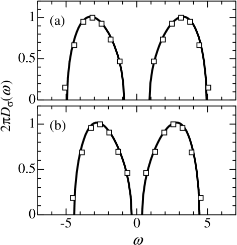
Figure 4: Density of states, $D_{\sigma}(\omega)=D(\omega)/2$, as obtained from the $1/U$ expansion, eq. (54), and the FE-ED for $n_{s}=15$; (a) $U=6$, (b) $U=5$.

In Fig. 4 we compare the density of states of our FE-ED for $n_{s}=15$ with those of the $1/U$ expansion to second order. Both for $U=5$ and $U=6$ the agreement is very good. Our FE-ED thus allows us to determine the density of states quantitatively with increasing resolution as $n_{s}$ increases.

Aside from the fact that the $1/U$ expansion provides an educated guess for the position of the Hubbard bands, the FE-ED is an independent numerical method based on the DMFT. The good agreement of the results mutually supports the applicability of either method. Therefore, we are confident that neither of the limitations poses a serious problem for our investigation of the Mott–Hubbard insulator, i.e., the problem of convergence of the series expansions in $1/U$ and in $1/n_{s}$, respectively, are not too serious in our approaches.

5 Random Dispersion Approximation

In this section, we present numerical results from the Random Dispersion Approximation (RDA). This method is not based on the DMFT and thereby provides yet another independent check for the validity of our results as obtained in Sects. 3 and 4.

In the Random Dispersion Approximation, the dispersion relation $\epsilon(\vec{k})$ in the kinetic energy is replaced by a random quantity $\epsilon^{\rm RDA}(\vec{k})$ where the bare density of states acts as probability distribution,

$$\rho(\epsilon)=\frac{1}{L}\sum_{\vec{k}}\delta(\epsilon-\epsilon^{\rm RDA}(\vec{k}))\;.$$ (88)

This is the characteristic property of the dispersion relation in infinite dimensions Gebhardbook so that the RDA with the semi-elliptic density of states (6) becomes exact for the Bethe lattice with infinite coordination number in the thermodynamic limit $L\to\infty$.

All correlation functions factorize, analogously to (2.1). For the $m$th-order correlation function,

$$\rho_{1\ldots m}(\epsilon_{1},\ldots,\epsilon_{m})=\frac{1}{L}\sum_{\vec{k}}\prod_{l=1}^{m}\delta\left(\epsilon_{l}-\epsilon(\vec{k}+\vec{q}_{l})\right)\;,$$ (89)

we give a recursive algorithm. Let $\rho_{l}(\epsilon_{l})\equiv\rho(\epsilon_{l})$ be the bare density of states, for $m=2$, see (2.1), and for $m\geq 3$ we define

$$\rho_{1\ldots(n-1);n,\ldots,m}(\epsilon_{1},\ldots,\epsilon_{m}) = \prod_{i,j=n}^{m}(1-\delta_{\vec{q}_{i},\vec{q}_{j}})$$

$$\prod_{i=n}^{m}\prod_{j=1}^{n-1}(1-\delta_{\vec{q}_{i},\vec{q}_{j}})$$

$$\rho_{1\ldots m}(\epsilon_{1},\ldots,\epsilon_{m})\;.$$

In this quantity, all $\vec{q}_{l}$ for $l\geq n$ are pairwise different, and they are also different from those $\vec{q}_{i}$ with $i\leq n-1$. The recursion formula

$$\rho_{1\ldots n;(n+1),\ldots,m}(\epsilon_{1},\ldots,\epsilon_{m})=$$

$$\rho_{1\ldots(n-1);n,\ldots,m}(\epsilon_{1},\ldots,\epsilon_{m})$$

$$+\left[1-\prod_{l=1}^{n-1}\left(1-\delta_{\vec{q}_{n},\vec{q}_{l}}\delta(\epsilon_{n}-\epsilon_{l})\right)\right]$$

$$\times\rho_{1\ldots(n-1);(n+1),\ldots,m}(\epsilon_{1},\ldots,\epsilon_{n-1},\epsilon_{n+1},\ldots,\epsilon_{m})$$

starts with $\rho_{1\ldots m}(\epsilon_{1},\ldots\epsilon_{m})\equiv\rho_{1\ldots m;}(\epsilon_{1},\ldots\epsilon_{m})$ and terminates at

$$\rho_{1;2,\ldots,m}(\epsilon_{1},\ldots\epsilon_{m})=\prod_{l=1}^{m}\rho(\epsilon_{l})\prod_{i,j=1}^{m}(1-\delta_{\vec{q}_{i},\vec{q}_{j}})\;.$$ (92)

For example,

$$\rho_{123}(\epsilon_{1},\epsilon_{2},\epsilon_{3}) = \Bigl{[}1-\prod_{l=1}^{2}\left(1-\delta_{\vec{q}_{3},\vec{q}_{l}}\delta(\epsilon_{3}-\epsilon_{l})\right)\Bigr{]}\rho_{12}(\epsilon_{1},\epsilon_{2})$$ (93)

$$+\rho_{12;3}(\epsilon_{1},\epsilon_{2},\epsilon_{3})$$

with

$$\rho_{12;3}(\epsilon_{1},\epsilon_{2},\epsilon_{3}) = \delta_{\vec{q}_{1},\vec{q}_{2}}\delta(\epsilon_{1}-\epsilon_{2})\rho(\epsilon_{1},\epsilon_{3})$$

$$+\rho(\epsilon_{1})\rho(\epsilon_{2})\rho_{(}\epsilon_{3})$$

$$\times(1-\delta_{\vec{q}_{1},\vec{q}_{2}})(1-\delta_{\vec{q}_{1},\vec{q}_{3}})(1-\delta_{\vec{q}_{2},\vec{q}_{3}})\;.$$

In order to put the RDA into practice, we choose a one-dimensional lattice of $L$ sites in momentum space

$$k_{\ell}=\frac{2\pi}{L}\left(-\frac{L+1}{2}+\ell\right)\;(\ell=1,\ldots,L)\;,$$ (95)

and determine the dispersion relation $\epsilon(k)$ as the solution of the implicit equation

$$k/2=\left(2\epsilon(k)/W\right)[1-\left(2\epsilon(k)/W\right)^{2}]^{1/2}+\arcsin\left(2\epsilon(k)/W\right)\;.$$ (96)

This choice guarantees $\rho(\epsilon)=\rho_{0}(\epsilon)$ in the thermodynamic limit.

Next, we choose a permutation ${\cal Q}_{\sigma}$ for each spin direction $\sigma$ which permutes the sequence $\{1,\ldots,L\}$ into $\{{\cal Q}_{\sigma}[1],\ldots,{\cal Q}_{\sigma}[L]\}$; in this way there are $(L!)^{2}$ independent realizations for a given finite $L$. A specific realization of the RDA dispersion is then defined by ${\cal Q}=[{\cal Q}_{\uparrow},{\cal Q}_{\downarrow}]$. Then, the numerical task is the Lanczos diagonalization of the Hamiltonian

$$\hat{H}^{{\cal Q}}=\sum_{\sigma}\sum_{\ell=1}^{L}\epsilon(k_{{\cal Q}_{\sigma}[\ell]})\hat{c}_{k_{\ell},\sigma}^{+}\hat{c}_{k_{\ell},\sigma}+U\hat{D}\;.$$ (97)

In this way we obtain the ground-state energy $E_{0}^{\cal Q}(N;U)$, the single-particle gap

$$\Delta^{\cal Q}(U)=2[E_{0}^{\cal Q}(N=L+1;U)-E_{0}^{\cal Q}(N=L;U)]\;,$$ (98)

and the momentum distribution

$$n^{\cal Q}(\epsilon;U)=\frac{1}{2}\sum_{\sigma}\left.\vphantom{\sum}\langle\hat{n}_{k_{\ell},\sigma}\rangle\right|_{\epsilon(k_{\ell})=\epsilon}\;,$$ (99)

where $\langle\ldots\rangle$ denotes the ground-state expectation value for the realization ${\cal Q}$.

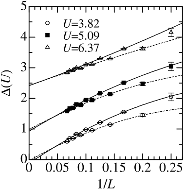
Figure 5: Gap as a function of system size ($L\leq 15$) in the Random Dispersion Approximation for various values of the interaction strength. The extrapolations are done for even and odd system sizes separately.

As a next step, we obtain all physical quantities for fixed system size $L$ by averaging over the number $N_{\cal Q}$ of realizations ${\cal Q}$. Typically, we choose at least $N_{\cal Q}=100$ for $6\leq L\leq 16$. For the physical quantities we obtain gaussian-shaped distributions for which we can determine the average values, e.g.,

$$\Delta(U) = \frac{1}{N_{\cal Q}}\sum_{{\cal Q}}\Delta^{\cal Q}(U)\;,$$ (100)

$$n(\epsilon;U) = \frac{1}{N_{\cal Q}}\sum_{{\cal Q}}n^{\cal Q}(\epsilon;U)$$ (101)

with accuracy ${\cal O}(1/N_{\cal Q})$.

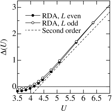
Figure 6: Gap in RDA as a function of the interaction strength. Filled symbols: extrapolation from even $L$, open symbols: extrapolation from odd $L$. Also shown is the result from second-order perturbation theory in $1/U$ (58).

In order to improve slightly the quality of our distributions, we impose a filter on our randomly chosen permutations. For a truly random dispersion, $L|t^{\rm RDA}(\ell)|^{2}=\overline{\epsilon^{2}}$ is independent of $\ell$; see (35). Therefore, we discard those realizations for which

$$\sum_{\ell=1}^{L-1}\left[|t^{{\cal Q}_{\sigma}}(\ell)|^{2}-\overline{\epsilon^{2}}\right]^{2}>d_{L}$$ (102)

with, $d_{L}\approx 0.2$ for $L\leq 16$. In this way we admit about every second of the randomly chosen configurations. Note that there are of the order of $(L!)^{2}$ different realizations so that our filter does not introduce any unwanted bias.

In Fig. 5 we show the gap as calculated from (98). Typically, the statistical errors are of the symbol size or smaller. Due to the sizable odd-even effect, we extrapolate the data for odd and even $L$ separately. This gives another check on the influence of finite-size effects. It is seen that the behavior as a function of $1/L$ is quite regular, i.e., the finite-size gap behaves as in generic many-body problems.

In Fig. 6 we show the result of an extrapolation of the finite-size data for even and odd system sizes. We consider the agreement with the $1/U$ expansion as quite acceptable for $U>U_{\rm c}$ which we can estimate as

$$U_{\rm c}^{\rm RDA}=4.0\pm 0.4\;.$$ (103)

Finite-size effects result in a smearing of the gap at the transition, and a gap exponent cannot be determined. However, the fact that the extrapolated gap turns slightly negative can be taken as an indication that the gap opens at $U_{\rm c}$ with an exponent not too far from unity.

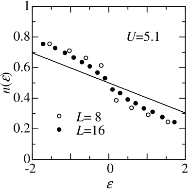
Figure 7: Momentum distribution in RDA for $U=16/\pi\approx 5.1$ for the two largest system sizes. The full line is the result from first-order perturbation theory in $1/U$ (72).

Lastly, in Fig. 7 we show the momentum dispersion within the RDA for $U=16/\pi\approx 5.1$, together with the result of the $1/U$ expansion. Obviously, there are large finite-size effects which make a finite-size extrapolation difficult. The reason for this behavior is related to the fact that all finite-size systems appear to have a finite discontinuity at the Fermi energy as well as a finite single-particle gap. For insulators, the apparent jump in $n(\epsilon)$ only vanishes in the thermodynamic limit RDA . The agreement between the RDA data and the momentum distribution as obtained from the $1/U$ expansion is good enough to argue that the RDA will eventually converge to the $1/U$ result for $L\to\infty$.

The RDA becomes exact for lattice electrons in high dimensions. In contrast to the FE-ED it is not based on the DMFT self-consistency equations. Moreover, it does not require the convergence of the $1/U$ expansion. Despite the observed limitations in accuracy, the results from RDA confirm of our findings in Sects. 3 and 4: the $1/U$ expansion and the FE-ED provide an accurate description of the Mott–Hubbard insulator whose gap opens at the critical interaction strength $U_{\rm c}=4.43\pm 0.05$.

6 Comparison with analytic approximations

In this section we compare our results with two analytic approximations to the DMFT which become exact for the Bethe lattice in the strong-coupling limit, i.e., they reproduce $D_{\rm LHB}(\omega)$ to order $(1/U)^{0}$. The Local Moment Approach (LMA) LMA outlined in appendix B fulfills this condition by construction, whereas this is a non-trivial result within the Iterated Perturbation Theory (IPT) iptoriginal ; a proof Mikethesis is given in appendix A.

The Hubbard-III approximation HubbardIII also fulfills this criterion but it fails to reproduce qualitatively the density of states for smaller interaction strengths Eva . Therefore, we do not further discuss the Hubbard-III approximation.

6.1 Iterated Perturbation Theory

For the $Z\to\infty$ Bethe lattice, the self-energy and the local single-particle Green function are related by

$$G_{\sigma}(\omega)=\frac{1}{\omega-G_{\sigma}(\omega)-\Sigma_{\sigma}(\omega)}.$$ (104)

In IPT, the self-energy is approximated by

$$\Sigma_{\sigma}(\omega)=U^{2}\int_{-\infty}^{\infty}\frac{{\rm d}\Omega}{2\pi{\rm i}}\Pi(\Omega){\cal G}_{\sigma}(\omega-\Omega)\;.$$ (105)

Here ${\cal G}_{\sigma}(\omega)$ is the host Green function,

$${\cal G}_{\sigma}(\omega)=\frac{1}{\omega-G_{\sigma}(\omega)},$$ (106)

and we have defined the polarization bubble

$$\Pi(\omega)=-\int_{-\infty}^{\infty}\frac{{\rm d}\omega_{1}}{2\pi{\rm i}}{\cal G}_{\sigma}(\omega_{1}){\cal G}_{\sigma}(\omega_{1}-\omega)$$ (107)

in terms of the host Green function.

It is helpful to consider the low-frequency behavior of the IPT equations. First, consider the host Green function (106), whose low-frequency behavior in the insulator is given generally by

$${\cal G}_{\sigma}(\omega)=\frac{\left|{m_{0}}\right|}{\omega+{\rm i}\eta\,{\rm sgn}(\omega)}\qquad\omega\to 0\>,$$ (108)

where the pole weight $\left|{m_{0}}\right|$ is given in terms of

$$|\gamma_{1}|=-\left.\frac{{\rm d}G_{\sigma}(\omega)}{{\rm d}\omega}\right|_{\omega=0}$$ (109)

as

$$\left|{m_{0}}\right|=(1+\left|\gamma_{1}\right|)^{-1}\;.$$ (110)

${\cal G}_{\sigma}(\omega)$ also contains a Hubbard-band contribution, which is strictly separated from the pole at $\omega=0$ throughout the insulating phase, whence we may write

$${\cal G}_{\sigma}(\omega)={\cal G}_{\sigma}^{\rm band}(\omega)+\frac{\left|{m_{0}}\right|}{\omega+{\rm i}\eta\,{\rm sgn}(\omega)}\;,$$ (111)

which actually defines ${\cal G}_{\sigma}^{\rm band}(\omega)$. In IPT the low-frequency behavior of ${\cal G}_{\sigma}(\omega)$ directly determines the low-frequency behavior of $\Sigma_{\sigma}(\omega)$; inserting (111) into (105) and (107) yields

$$\Sigma_{\sigma}(\omega)=\frac{A}{\omega}\qquad\omega\to 0\>,$$ (112)

where

$$A=\frac{U^{2}}{4}\left|{m_{0}}\right|^{3}\;.$$ (113)

To satisfy self-consistency (104) requires

$$A=\frac{1}{\left|\gamma_{1}\right|}\;,$$ (114)

so that (110), (113) and (114) determine the low-frequency behavior of the problem. In particular, they yield

$$\frac{2}{\left|{m_{0}}\right|\sqrt{1-\left|{m_{0}}\right|}}=U\;.$$ (115)

The denominator ${\left|{m_{0}}\right|\sqrt{1-\left|{m_{0}}\right|}}$ reaches its maximum value when

$$\left|{m_{0}}\right|=\left|{m_{0}^{\rm min}}\right|=\frac{2}{3}\;,$$ (116)

thus locating the destruction of the Mott–Hubbard insulator at

$$U_{{\rm c},1}^{\rm IPT}=3\sqrt{3}\approx 5.2\;,$$ (117)

as earlier reported by Rozenberg et al. KotliarIPT . The IPT prediction lies considerably above our best estimate $U_{\rm c}=4.43\pm 0.05$.

Figure 8: Gap as a function of interaction strength from second-order perturbation theory in $1/U$ (58), the Fixed-Energy Exact Diagonalization (FE-ED), the Local Moment Approach (LMA), and Iterated Perturbation Theory (IPT).

Figure 9: Density of states for $U=6$ in Iterated Perturbation Theory (solid line) and in second-order perturbation theory in $1/U$ (54) (dashed line).

This discrepancy can already be seen for larger interaction strength where

$$\Delta^{\rm IPT}(U)=U-4-\frac{5}{2U}-\ldots\;.$$ (118)

The first-order correction can be obtained analytically, as shown in appendix A. It is more than twice as large as our exact coefficient. Therefore, the agreement is good only for $U>6$. The gap in IPT is compared to our FE-ED and second-order results in Fig. 9. As seen from the figure, and shown analytically in Mikethesis , the gap closes continuously but with an exponent of $\gamma_{\rm IPT}=1/2$.

Despite the deviations in the gap values, the IPT correctly reproduces the overall shape of the density of states for $U>6$, apart from the artificial high-energy tails of the IPT Hubbard bands. The threshold exponent for the density of states is correct, $\alpha_{\rm IPT}=1/2$ in the Mott–Hubbard insulator. Nevertheless, the deviations from the second-order result (54) are quite noticeable at $U=6$ which is shown in Fig. 9. We conclude that the IPT provides a quantitatively correct description of the Mott–Hubbard insulator down to $U\approx 6$. However, IPT seriously underestimates the stability of the Mott–Hubbard insulator.

6.2 Local Moment Approach

Details of the LMA are given in Ref. LMA . As shown in appendix B, the LMA gap to first order in $1/U$ is given by

$$\Delta^{\rm LMA}(U)=U-4-\frac{3}{2U}\;.$$ (119)

The first-order correction is close to the exact one, and, correspondingly, the agreement with our strong-coupling result (58) is very good down to $U\approx 5.5$. For smaller interaction strengths, the deviations become noticeable and the LMA predicts the collapse of the insulator to occur at $U_{\rm c}^{\rm LMA}=4.82$ LMA which is larger than our best estimate $U_{\rm c}=4.43\pm 0.05$. The LMA yields a critical gap exponent $\gamma_{\rm LMA}=1$ Mikethesis , in contrast to IPT where $\gamma_{\rm IPT}=1/2$. The gap in LMA and our second-order and FE-ED results are shown in Fig. 9.

It is seen that the LMA gap is more accurate than the gap from IPT. In particular, this holds true for the density of states as the LMA very well reproduces our second-order result (54). The comparison for $U=4\sqrt{2}\approx 5.66$ is shown in Fig. 10. The deviations are largest around the gap. The overall agreement, however, is excellent. In particular, the threshold exponent is $\alpha_{\rm LMA}=1/2$.

Figure 10: Density of states for $U=4\sqrt{2}\approx 5.66$ from the Local Moment Approach (full line) and second-order perturbation theory in $1/U$ (54) (dashed line). On the scale of the figure, the gap from FE-ED and from second-order perturbation theory are almost the same.

The LMA thus provides a qualitatively correct description of the Mott–Hubbard insulator. It is a quantitatively reliable approximation down to $U\approx 5.5$.

7 Other numerical approximations to the DMFT

In this section we discuss two other exact-diagonalization approaches. In both of them a discretized version of the single-impurity Anderson model (SIAM), Sect. 4.1, is investigated in which the site energies $\epsilon_{\ell}$ are determined self-consistently. This is the decisive difference to our ‘fixed-energy’ algorithm as presented in Sect. 4.

In this work, we do not discuss the Numerical Renormalization Group (NRG) approach to the Mott–Hubbard insulator. The NRG is custom-tailored for the description of the metallic phase in the sense that it tries to resolve structures around $\omega=0$ whereas features at high energies are broadened on a logarithmic scale BullaPRL . Therefore, the Mott–Hubbard insulator does not display a clear gap. Consequently, as can be seen from Fig. 2 in Ref. BullaPRL , the density of states is finite in the gap, and the NRG Hubbard bands display sizable high-energy tails. Therefore, the gap and the width of the Hubbard bands as a function of the interaction strength cannot be easily deduced from this approach.

7.1 Exact diagonalization in ‘two-chain geometry’

In contrast to Sect. 4.1, an alternative formulation of the Hamilton operator for the SIAM describes two chains of length $(n_{s}-1)/2$ which represent the upper and lower Hubbard bands. They are coupled to the impurity site at the respective chain origins RMP ; Rozenbergetal

$$\hat{H}_{\rm SIAM-tc} = \sum_{\ell=1;\sigma}^{(n_{s}-1)/2}\epsilon_{\ell}\left(\hat{u}_{\sigma;\ell}^{+}\hat{u}_{\sigma;\ell}-\hat{l}_{\sigma;\ell}^{+}\hat{l}_{\sigma;\ell}\right)$$

$$+U\left(\hat{d}_{\uparrow}^{+}\hat{d}_{\uparrow}-\frac{1}{2}\right)\left(\hat{d}_{\downarrow}^{+}\hat{d}_{\downarrow}-\frac{1}{2}\right)$$

$$+\sum_{\sigma}\sqrt{\frac{1}{2}}\left(\hat{u}_{\sigma;1}^{+}\hat{d}_{\sigma}+\hat{l}_{\sigma;1}^{+}\hat{d}_{\sigma}+{\rm h.c.}\right)$$

$$+\sum_{\ell=1}^{(n_{s}-3)/2}\!\!\!V_{\ell}\left(\hat{u}_{\sigma;\ell+1}^{+}\hat{u}_{\sigma;\ell}+\hat{l}_{\sigma;\ell+1}^{+}\hat{l}_{\sigma;\ell}+{\rm h.c.}\right)\;.$$

Here particle-hole symmetry results in $\epsilon_{\ell}>0$ for $\ell=1,\ldots,(n_{s}-1)/2$, and $V_{\ell}>0$ for $\ell=1,\ldots,(n_{s}-3)/2$.

The main advantage of the two-chain geometry lies in the fact that on the Bethe lattice the self-consistency condition (78) can be implemented exactly even for finite $n_{s}$. In the continued-fraction expansion of the Green function for the Hubbard bands (13), the local energies $\epsilon_{\ell}$ and the electron transfer amplitudes $V_{\ell}$ appear as diagonal and off-diagonal coefficients,

$$G_{\rm LHB;\sigma}(\omega)=\frac{1/2}{\omega+U/2-(V_{1})^{2}/[\omega-\epsilon_{1}-\ldots]}\;.$$ (121)

The (dynamical) Lanczos procedure directly provides the continued-fraction coefficients so that the output of the exact diagonalization procedure yields the input for the next iteration of the self-consistency cycle without a collection of weights as, e.g., in (81).

For this reason, the two-chain ED is rather appealing. Moreover, using the results for $n_{s}=3,5,7$ and some unspecified extrapolation in $1/n_{s}$, the gap in RMP was found to be almost linear as a function of the interaction strength above $\widetilde{U}_{\rm c}=4.30$, in surprisingly good agreement with our best estimate (87). The corresponding results for $n_{s}=3,5,7$ are shown in Fig. 11. If we take only those three data points into account and assume a linear scaling in $1/n_{s}$, we obtain the gap as shown in Fig. 12 which is very similar to the result reported in RMP , and is in reasonable agreement with the results from the $1/U$ expansion. Thus, one would be tempted to conclude that the method is quite reliable. Unfortunately, such a conclusion is not warranted.

Figure 11: Gap in exact diagonalization of the single-impurity model in two-chain geometry for $n_{s}=3,5,7$ for various interactions $U$. The lines are a linear extrapolation to $1/n_{s}\to 0$.

Figure 12: Extrapolated gap (see Fig. 11) in the exact diagonalization of the single-impurity model in two-chain geometry as a function of the interaction strength, as compared to second-order perturbation theory in $1/U$ (58).

Figure 13: Gap in exact diagonalization of the single-impurity model in two-chain geometry for $n_{s}\leq 13$ for various interactions $U$. The lines are a cubic spline extrapolation to $1/n_{s}\to 0$.

Figure 14: Extrapolated gap (see Fig. 13) in the exact diagonalization of the single-impurity model in two-chain geometry as a function of the interaction strength, as compared to second-order perturbation theory in $1/U$ (58).

First, bigger system sizes need to be analyzed because $n_{s}=3,5,7$ correspond to chain lengths of $L_{\rm c}=1,2,3$. When we follow the original algorithm as described in Rozenbergetal , we find that the insulating phase becomes unstable at $U=8$ for $n_{s}=13$ ($U=6.4,5.0,3.5$ for $n_{s}=11,9,7$). Obviously, this is a numerical artifact which is not related to the metal-insulator transition. We have found that this problem can be cured by incorporating the particle-hole symmetry into $\hat{H}_{\rm SIAM-tc}$ (7.1) right from the start; this was done only ‘on average’ in Ref. Rozenbergetal . In the following, we show results obtained using this particle-hole symmetry.

When we include bigger system sizes, we obtain a behavior quite different from the one seen in Fig. 12. The result for the gap as a function of $1/n_{s}$ for $n\leq 13$ is shown in Fig. 13. The behavior of the gap as a function of $1/n_{s}$ can no longer be approximated by a linear fit. The gap is not regular as a function of $1/n_{s}$ but seems to saturate. When we interpolate using a cubic spline, we obtain the gap as a function of the interaction strength as shown in Fig. 14. Obviously, the results are rather poor as the large-$U$ limit cannot be reproduced properly and there is nowhere agreement with the results from the $1/U$ expansion. It is thus seen that the agreement between the data reported in RMP ; andere and ours is fortuitous.

Figure 15: Density of states as obtained from the two-chain exact diagonalization for $U=6$ and $n_{s}=13$ (full line), as compared to second-order perturbation theory in $1/U$ (54) (dashed line).

The poor quality of the two-chain ED is also seen in the density of states, as shown in Fig. 15 for $n_{s}=13$ and $U=6$. For all $n_{s}\geq 7$ we obtain a four-peak structure which does not allow the recovery of the true density of states.

The reason for the failure of the method lies in the setup of the self-consistency scheme. In the continued-fraction expansion one optimizes the moments of the density of states. However, the reconstruction of the density of states from its moments is a numerically very delicate inverse problem. In our case, the moments of the upper Hubbard band can be approximated very well by three main peaks and many small peaks at (much) higher energy. For this reason, the structure of the density of states is essentially unchanged as a function of $n_{s}$. The convergence as a function of system size saturates, and a reliable extrapolation scheme is not evident. We thus conclude that the two-chain ED is not a suitable tool for the investigation of the Mott–Hubbard insulator.

7.2 Caffarel–Krauth exact diagonalization in ‘star geometry’

As an alternative to the two-chain discretization of the previous section, Caffarel and Krauth used the discretization of the single-impurity Anderson model in ‘star geometry’ (73). In contrast to our FE-ED, both the hybridization parameters $V_{\ell}$ and the site energies $\epsilon_{\ell}$ are determined self-consistently in the Caffarel–Krauth scheme (CK-ED).

In order to close the self-consistency cycle, a $\chi^{2}$-fitting procedure CK ; Ono is used. Let $T$ be a fictitious small temperature, typically $T=1/200$, and $\omega_{n}=(2n+1)\pi T$ are the corresponding Matsubara frequencies. For a given parameter set $(\epsilon_{\ell},V_{\ell})$ we solve the single-impurity model for the single-particle Green function $G_{\sigma}^{(n_{s})}(\omega)$. Then, the self-consistency equation (78) allows us to deduce the parameter set for the next iteration from the minimization of

$$\chi^{2}(\epsilon_{\ell}^{\rm new},V_{\ell}^{\rm new}) = \sum_{n=0}^{n_{\rm M}}\Bigl{|}H^{(n_{s})}({\rm i}\omega_{n};\epsilon_{\ell}^{\rm new},V_{\ell}^{\rm new})$$ (122)

$$\hphantom{\sum_{n=0}^{n_{\rm M}}\Bigl{|}}-G_{\sigma}^{(n_{s})}({\rm i}\omega_{n};\epsilon_{\ell},V_{\ell})\Bigr{|}^{2}\;.$$

Here $n_{\rm M}$ is a (large) upper cut-off.

Figure 16: Density of states for $U=6$ as obtained from the $1/U$ expansion (solid line), in comparison with two converged solutions of the Caffarel–Krauth Exact Diagonalization scheme (CK-ED) for $n_{s}=11$ sites (solid points).

In Fig. 16 we show two typical converged results for the density of states for $U=6$, starting from two different initial values for the set $(V_{\ell},\epsilon_{\ell})$. Note that the solutions are not unique, i.e., there are many self-consistent solutions for the insulator. At first glance, the two solutions appear to be very similar. The main peaks have almost the same weights $V_{\ell}^{2}$ and the same positions $\epsilon_{\ell}$. This can be expected because the main peaks dominate $\chi^{2}$ in (122). Moreover, the overall distribution of weights and energies by and large follows the true density of states from the analytical calculation.

A closer look into the figures reveals a fundamental problem. In Fig. 16a the first non-vanishing peak appears at $\Delta_{a}^{(11)}(6)/2=0.966$ whereas in Fig. 16b the value for half the gap is estimated as $\Delta_{b}^{(11)}(6)/2=1.06$. The same results follow if we use the difference of the ground-state energies (82) for the definition of the gap. Obviously, we cannot give a unique value for $\Delta^{{\rm CK-ED};(n_{s})}$, and an extrapolation $n_{s}\to\infty$ is impossible. The reason for this problem lies in the fact that the peak at the onset of the density of states is rather small so that its precise position and weight do not matter much in the $\chi^{2}$-fit (122). Thus, the onset energy may easily fluctuate by 10% or more, as seen in Fig. 16. Therefore, the CK-ED approach cannot provide a reliable estimate for the gap.

The failure of the self-consistency can be traced back to the fact that, for general filling, the Green function $G^{(n_{s})}(\omega)$ contains only $n_{s}$ poles with substantial weight whereas $H^{(n_{s})}(\omega)$ is characterized by $(2n_{s})$ parameters $(\epsilon_{\ell},V_{\ell}^{2})$ in the CK-ED. Too much flexibility in the hybridization function leads to non-unique solutions of the self-consistency equations. Our Fixed-Energy Exact Diagonalization cures this problem because only $n_{s}$ parameters $V_{\ell}^{2}$ are to be determined.

8 Conclusions

In this work, we have studied the insulating phase of the half-filled Hubbard model on a Bethe lattice with infinite connectivity (band-width $W=4t$). As long as the strong-coupling perturbation theory converges, the ground state of the Mott–Hubbard insulator has a finite entropy density, $s=\ln(2)$, and the density of states of the lower and upper Hubbard bands increases as a function of frequency with the edge exponent $\alpha=1/2$, see (56). Furthermore, we find that the high-order corrections to the gap as a function of $1/U$ are fairly small. Thus, the gap opens at the critical interaction strength $U_{\rm c}^{\rm sc}=4.40\pm 0.09$. Our explicit results to second order in $1/U$ (54) provide a benchmark test for analytical and numerical approaches to the Mott–Hubbard insulator in infinite dimensions.

We have used our results from the $1/U$ expansion to set up a new numerical scheme for the effective single-impurity Anderson model in the Dynamical Mean-Field Theory. In our Fixed-Energy Exact Diagonalization (FE-ED), we start an outer self-consistency cycle with the position and width of the Hubbard bands from perturbation theory which we resolve equidistantly to accuracy $9t/(n_{s}-1)$ for $n_{s}\leq 15$. The extrapolation $n_{s}\to\infty$ thereby becomes systematic. In an inner self-consistency cycle we determine the hybridization strengths for given $n_{s}$ using a dynamical Lanczos procedure. From this we determine the gap after extrapolation to the thermodynamic limit. We merge the extrapolated gap from the ‘energy criterion’ and the ‘weight criterion’ in order to obtain a new estimate for the onset of the Hubbard bands. In this way, we iterate to convergence the outer self-consistency cycle.

Our FE-ED very well reproduces the gap, the density of states, and the exponent $\alpha=1/2$ from perturbation theory. In this way we confirm our estimate for the transition to $U_{\rm c}^{\rm FE-ED}=4.43\pm 0.05$. As a last check, we favorably compare our results with those from the Random Dispersion Approximation which is an independent approach to the limit of infinite dimensions. Thus, we are confident that the strong-coupling perturbation theory, our Fixed-Energy Exact Diagonalization scheme for the Dynamical Mean-Field Theory, and the Random Dispersion Approximation provide a consistent and accurate description of the Mott–Hubbard insulator.

Other analytical and numerical techniques for the solution of the Dynamical Mean-Field Theory meet our benchmark test with limited success. The best analytical approximation is the Local Moment Approach which is quantitatively reliable for the density of states down to $U=5.5$; it reproduces the correct exponent $\alpha=1/2$ but overestimates the critical interaction strength, $U_{\rm c}^{\rm LMA}=4.8$. Iterated Perturbation Theory reproduces the correct threshold exponent $\alpha=1/2$ but it becomes quantitatively and qualitatively unreliable below $U=6$ and underestimates the stability of the Mott–Hubbard insulator, $U_{\rm c}^{\rm IPT}=5.2$.

Of the two exact-diagonalization (ED) schemes for the effective single-impurity problem existing in the literature, the two-chain approach fails because it leads to an ill-conditioned inverse problem, namely, the recovery of the density of states from its moments. The Caffarel–Krauth exact diagonalization approach (CK-ED) in star geometry gives a reasonable guess for the shape of the density of states, but it fails to provide a reliable estimate for the gap. For fixed system size, the fitting procedure results in different solutions with noticeable differences for the onset of the density of states. Therefore, it is not possible to set up a sensible extrapolation scheme for $n_{s}\to\infty$.

In this work we have presented a qualitatively and quantitatively reliable analysis of the Mott–Hubbard insulator. It will provide a solid basis for further studies of the Mott–Hubbard metal-insulator transition.

Acknowledgments

We thank Eric Jeckelmann and David Logan for helpful discussions. Support by the Deutsche Forschungsgemeinschaft (GE 746/5-1+2) and the center Optodynamics of the Philipps-Universität Marburg is gratefully acknowledged. We thank the HRZ Darmstadt computer facilities where some of the calculations were performed.

Appendix A Iterated Perturbation Theory (IPT) in strong coupling

We here write the IPT self-energy, cf. (104)–(107), in a form amenable to numerical calculations and additionally find its strong coupling form. We start by rearranging (111) as follows

$${\cal G}_{\sigma}(\omega) = {\cal G}_{\sigma}^{\rm band}(\omega)+\frac{\left|{m_{0}}\right|}{\omega+{\rm i}\eta\,{\rm sgn}(\omega)}$$ (123)

$$= {\cal G}_{\sigma,+}^{\rm band}(\omega)+{\cal G}_{\sigma,-}^{\rm band}(\omega)+\frac{\left|{m_{0}}\right|/2}{\omega-{\rm i}\eta}+\frac{\left|{m_{0}}\right|/2}{\omega+{\rm i}\eta}$$

$$+\frac{{\rm i}\pi}{2}\left|{m_{0}}\right|\left(\delta(\omega-0^{-})-\delta(\omega-0^{+})\right)\>,$$

where ${\cal G}_{\sigma,\pm}^{\rm band}(\omega)$ are the retarded/advanced components of ${\cal G}_{\sigma}^{\rm band}(\omega)$. Inserting (123) into (107), and performing a simple contour integration, yields for $\Pi(\omega)$

$$\Pi(\omega) = \frac{(\left|{m_{0}}\right|/2)^{2}}{\omega-{\rm i}\eta}-\frac{(\left|{m_{0}}\right|/2)^{2}}{\omega+{\rm i}\eta}$$ (124)

$$+ \left|{m_{0}}\right|\left\{{\cal G}_{\sigma,-}^{\rm band}(\omega)-{\cal G}_{\sigma,+}^{\rm band}(\omega)\right\}+I_{1}(\omega)\>,$$

where

$$I_{1}(\omega)=-\int_{-\infty}^{\infty}\frac{{\rm d}\omega_{1}}{2\pi{\rm i}}{\cal G}_{\sigma}^{\rm band}(\omega_{1}){\cal G}_{\sigma}^{\rm band}(\omega_{1}-\omega)\;.$$ (125)

Note that $\Im\Pi(\omega)$ has a pole contribution at $\omega=0$, specifically

$$\Pi(\omega)=\frac{{\rm i}\pi}{2}\left|{m_{0}}\right|^{2}\delta(\omega)+\Pi^{\rm band}(\omega)\;,$$ (126)

with

$$\Pi^{\rm band}(\omega)=\left|{m_{0}}\right|\left\{{\cal G}_{\sigma,-}^{\rm band}(\omega)-{\cal G}_{\sigma,+}^{\rm band}(\omega)\right\}+I_{1}(\omega)\;.$$ (127)

Insertion of (123) and (124) into (105) yields for the self-energy

$$\Sigma_{\sigma}(\omega) = U^{2}\left(\frac{\left|{m_{0}}\right|}{2}\right)^{2}\left\{3{\cal G}^{\rm band}(\omega)+\frac{\left|{m_{0}}\right|}{\omega+{\rm i}\eta\,{\rm sgn}(\omega)}\right\}$$ (128)

$$+ I_{2}(\omega)+\frac{\left|{m_{0}}\right|}{2}U^{2}\left\{I_{1}^{-}(\omega)-I_{1}^{+}(\omega)\right\}\;,$$

where

$$I_{2}(\omega)=U^{2}\int_{-\infty}^{\infty}\frac{{\rm d}\omega_{1}}{2\pi{\rm i}}{\cal G}_{\sigma}^{\rm band}(\omega-\omega_{1})\Pi^{\rm band}(\omega_{1})$$ (129)

and

$$I_{1}^{\pm}(\omega)=\pm\frac{1}{\pi}\int_{-\infty}^{\infty}\frac{{\rm d}\omega_{1}\Im I_{1}(\omega_{1})}{\omega_{1}-\omega\mp{\rm i}\eta}\;.$$ (130)

$\Im I_{1}(\omega)$ may be found using a convolution involving only $\Im{\cal G}_{\sigma}^{\rm band}(\omega)$, and likewise $\Im I_{2}(\omega)$ may be found from a convolution of $\Im{\cal G}_{\sigma}^{\rm band}(\omega)$ and $\Im\Pi^{\rm band}(\omega)$. For $\omega>0$,

$$\Im I_{1}(\omega) = \frac{1}{\pi}\int_{0}^{\omega}{\rm d}\omega_{1}\Im{\cal G}_{\sigma}^{\rm band}(\omega_{1})\Im{\cal G}_{\sigma}^{\rm band}(\omega-\omega_{1})\;,$$ (131)

$$\Im I_{2}(\omega) = \frac{U^{2}}{\pi}\int_{0}^{\omega}{\rm d}\omega_{1}\Im{\cal G}_{\sigma}^{\rm band}(\omega_{1})\Im{\Pi}^{\rm band}(\omega-\omega_{1})\;.$$

In order to calculate $\Im\Sigma_{\sigma}(\omega)$ for $\omega>0$, it is thus necessary, see (128), to perform only the two convolutions (131) and (LABEL:convol2), $\Im\Sigma_{\sigma}(\omega)$ for $\omega<0$ follows immediately by symmetry, whence $\Re\Sigma_{\sigma}(\omega)$ follows by Hilbert transform.

The above is what we implement numerically. However, when $U\to\infty$ eq. (128) simplifies. In this limit (115) gives $\left|{m_{0}}\right|\to 1$; note that $\left|{m_{0}}\right|\to 0$ is not a self-consistent possibility, since $\left|{m_{0}}\right|\geq 2/3$, cf. (116). Specifically,

$$\left|{m_{0}}\right|=1-\frac{4}{U^{2}}\quad,\quad U\to\infty\;.$$ (133)

Since $\left|{m_{0}}\right|$ is the weight of the pole in ${\cal G}_{\sigma}(\omega)$, (111), and $\int_{-\infty}^{\infty}\left|{\Im{\cal G}_{\sigma}(\omega)}\right|{\rm d}\omega=\pi$, we have

$$\Im{\cal G}_{\sigma}^{\rm band}(\omega)\sim{\cal O}(U^{-2})\quad,\quad U\to\infty\;.$$ (134)

Now, eqs. (131) and (LABEL:convol2) result in $I_{1}(\omega)\sim{\cal O}(U^{-4})$ and $I_{2}(\omega)\sim{\cal O}(U^{-2})$, whereby (128) reduces to

$$\Sigma_{\sigma}(\omega)=U^{2}\left(\frac{\left|{m_{0}}\right|}{2}\right)^{2}\left\{3{\cal G}_{\sigma}^{\rm band}(\omega)+\frac{\left|{m_{0}}\right|}{\omega+{\rm i}\eta\,{\rm sgn}(\omega)}\right\}\;,$$ (135)

with corrections ${\cal O}(U^{-2})$. Using (111) and  (106) this may be rewritten as

$$\Sigma_{\sigma}(\omega)=\frac{-3\left|{m_{0}}\right|^{2}U^{2}/4}{U/2-\omega^{\prime}+G_{\sigma}(\omega)}+\frac{U^{2}\left|{m_{0}}\right|^{3}/2}{U/2-\omega^{\prime}}+{\cal O}(U^{-2})\;,$$ (136)

where $\omega^{\prime}=\omega+U/2$. In the region of the lower Hubbard band only ($\omega^{\prime}\sim{\cal O}(1)$) eq. (136) may be expanded to give

$$\Sigma_{\sigma}(\omega) = -\frac{U}{2}-\omega^{\prime}+3G_{\sigma}(\omega)$$

$$-\frac{2}{U}\left[\omega^{\prime 2}-6\omega^{\prime}G_{\sigma}(\omega)+3G_{\sigma}(\omega)^{2}\right]+{\cal O}(U^{-2})\;.$$

If self-energy terms of ${\cal O}(U^{-1})$ and above are ignored, then $G_{\sigma}(\omega)$ in the region of the lower Hubbard band reduces to

$$G_{\sigma}(\omega)=\frac{1/2}{\omega^{\prime}-2G_{\sigma}(\omega)}\;,$$ (138)

and the single-particle density of states becomes

$$D_{{\rm LHB},\sigma}(\omega)=\frac{1}{4\pi}\sqrt{4-\omega^{\prime 2}}\;,$$ (139)

i.e., the correct strong coupling spectrum of a semi-ellipse with the full noninteracting band-width. Retaining the ${\cal O}(U^{-1})$ terms in eq. (A) gives the ${\cal O}(U^{-1})$ corrections to the position and shape of the LHB. The resultant spectrum is a distorted semi-ellipse of the form

$$D_{{\rm LHB},\sigma}(\omega) = \sqrt{4-\left(\omega^{\prime}-\frac{a_{\rm IPT}}{U}\right)^{2}+{\cal O}(U^{-2})}$$ (140)

$$\times\frac{1-(a_{\rm IPT}/U)\omega^{\prime}+{\cal O}(U^{-2})}{4\pi}\;,$$

where $a_{\rm IPT}=5/4$ and the LHB has band edges at $\omega^{\prime}=(a_{\rm IPT}/U)\pm 2$. The IPT result may be compared with the exact result to this order which also has the form of eq. (140) but with a different coefficient of $a=1/2$.

Appendix B Local Moment Approach (LMA) in strong coupling

The LMA of Logan et al. is described in detail in Ref. LMA , where it is proved that the LMA recovers the strong coupling single-particle spectrum up to and including terms of ${\cal O}(U^{0})$. Unlike IPT, the LMA also recovers the strong coupling spectrum in the antiferromagnetic phase LMA ; LMAPRL . The success of the LMA in strong coupling is unsurprising since the LMA is explicitly motivated by ideas of hole motion in a spin background. In this appendix we extend the previous analysis to recover the ${\cal O}(U^{-1})$ corrections to the LMA self-energy and single-particle spectrum in the strong-coupling limit. This is done in three stages. First the necessary equations of the LMA are given. Secondly, it is shown that only the coupling of hole motion to zero-frequency spin-flips survive, with the coupling of hole motion to higher energy particle-hole excitations only entering at ${\cal O}(U^{-2})$. Finally, the resultant self-energy is expanded to ${\cal O}(U^{-1})$ and the corresponding density of states is obtained.

The bare propagators within the LMA are unrestricted Hartree Fock (UHF) propagators. Lattice sites are taken to have up-spin or down-spin permanent local moments at random, and labeled ‘A-type’ or ‘B-type’ respectively. We focus solely on an A-type site (Green functions for B-type sites follow by symmetry) and suppress the ‘A’ labels in what follows. For the $Z=\infty$ Bethe lattice the UHF equations are simply

$$G_{\sigma}^{0}(\omega)=-G_{-\sigma}^{0}(-\omega)=[\omega+\frac{\sigma}{2}U\left|{\mu}\right|-G^{0}(\omega)]^{-1}\;,$$ (141)

where $\sigma=\pm 1$ for $\uparrow/\downarrow$ respectively, and the symmetric single-particle Green function obeys $G^{0}(\omega)=[G_{\uparrow}^{0}(\omega)+G_{\downarrow}^{0}(\omega)]/2$. The local moment is derived from

$$\mu = \int_{-\infty}^{0}{\rm d}\omega[D^{0}_{\uparrow}(\omega)-D^{0}_{\downarrow}(\omega)]\;,$$ (142)

$$D^{0}_{\sigma}(\omega) = -\frac{1}{\pi}{\rm sgn}(\omega)\Im G^{0}_{\sigma}(\omega)\;.$$ (143)

The RPA on-site particle-hole propagator

$$\Pi^{+-}(\omega)=\frac{\Pi^{+-}_{0}(\omega)}{1-U\Pi^{+-}_{0}(\omega)},$$ (144)

with

$$\Pi^{+-}_{0}(\omega)=-\int_{-\infty}^{\infty}\frac{{\rm d}\Omega}{2\pi{\rm i}}G_{\downarrow}^{0}(\Omega)G_{\uparrow}^{0}(\Omega-\omega)\;,$$ (145)

has a zero-frequency pole LMA (as well as higher-energy Stoner bands) reflecting the presence of zero-frequency spin-flip excitations in the system. In the full LMA single-particle Green function,

$$G_{\sigma}(\omega)=\left[\omega+\frac{\sigma}{2}U\left|{\mu}\right|-G(\omega)-\Sigma_{\sigma}(\omega)\right]^{-1},$$ (146)

hole motion and accompanying spin-flips are dynamically coupled via the self-energy

$$\Sigma_{\uparrow}(\omega)=-\Sigma_{\downarrow}(-\omega)=U^{2}\int\frac{{\rm d}\Omega}{2\pi{\rm i}}\Pi^{+-}(\Omega){\cal G}_{\downarrow}(\omega+\Omega).$$ (147)

The LMA equations must be solved self-consistently, since the host Green function reads

$${\cal G}_{\sigma}(\omega)=[\omega+\frac{\sigma}{2}U\left|{\mu}\right|-G(\omega)]^{-1}$$ (148)

with $G(\omega)=[G_{\uparrow}(\omega)+G_{\downarrow}(\omega)]/2$.

To calculate the LMA self-energy to ${\cal O}(U^{-1})$, we proceed in two stages. First we sketch the proof that only the zero-frequency spin-flip pole in $\Pi^{+-}(\omega)$ need be retained and the self-energy simplifies to

$$\Sigma_{\uparrow}(\omega) = U^{2}{\cal G}_{\downarrow}^{-}(\omega)+{\cal O}(U^{-2})$$ (149)

$$= U^{2}\int_{-\infty}^{0}\frac{{\rm d}\omega_{1}}{\pi}\frac{\Im{\cal G}_{\downarrow}(\omega_{1})}{\omega-\omega_{1}-{\rm i}\eta}+{\cal O}(U^{-2})\;.$$ (150)

Subsequently we analyze ${\cal G}_{\downarrow}^{-}(\omega)$ to obtain the spectrum to ${\cal O}(U^{-1})$.

It has been shown LMA that the RPA particle-hole propagator may be written

$$\Pi^{+-}(\omega)=\frac{Q}{-\omega-{\rm i}\eta}+\Pi^{+-}_{>}(\omega)+\Pi^{+-}_{<}(\omega)\;,$$ (151)

where $\Pi^{+-}_{>}(\omega)$ and $\Pi^{+-}_{<}(\omega)$ are the Stoner-like contributions whose imaginary parts are bands centered at $\pm U$ respectively. The full self-energy is thus

$$\Sigma_{\uparrow}(\omega)=QU^{2}{\cal G}_{\downarrow}^{-}(\omega)+\Sigma^{\rm S}_{\uparrow}(\omega)\;,$$ (152)

where

$$\Im\Sigma^{\rm S}_{\uparrow}(\omega)=\left\{\begin{array}[]{@{}lcl@{}}{-U^{2}\int_{0}^{\omega}{\rm d}\Omega{\cal D}_{\downarrow}(\Omega)\Im\Pi_{<}^{+-}(\Omega-\omega)}&\hbox{for}&\omega>0\\[6.0pt] {U^{2}\int_{\omega}^{0}{\rm d}\Omega{\cal D}_{\downarrow}(\Omega)\Im\Pi_{>}^{+-}(\Omega-\omega)}&\hbox{for}&\omega<0\end{array}\right.\,.$$ (153)

To show that $\Sigma^{\rm S}_{\uparrow}(\omega)\sim{\cal O}(U^{-2})$, it is necessary to examine $\Pi^{+-}(\omega)$ and hence $\Pi^{+-}_{0}(\omega)$ and $G_{\sigma}^{0}(\omega)$. By expanding $G_{\downarrow}^{0}(\omega)$ in the region of the LHB it quickly follows that

$$\left|{\mu}\right|=1-1/U^{2}+{\cal O}(U^{-3})\;.$$ (154)

Then $\Im\Pi^{+-}_{0}(\omega)$ may be shown from (145) to have a minority band centered around $\omega\approx-U$ with spectral weight $\left[(1-\left|{\mu}\right|)/2\right]^{2}=1/(4U^{4})+{\cal O}(U^{-5})$, and a majority band centered at $\omega\approx U$ with spectral weight $\left[(1+\left|{\mu}\right|)/2\right]^{2}=1-1/(U^{2})+{\cal O}(U^{-3})$. The bands of the RPA propagator which follow from (144),

$$\Im\Pi^{+-}(\omega)=\frac{\Im\Pi^{+-}_{0}(\omega)}{\left|{1-U\Pi^{+-}_{0}(\omega)}\right|^{2}}\;,$$ (155)

are also centered around $\omega=\pm U$. Since $\Pi^{+-}_{0}(\omega)\sim{\cal O}(1)$ in the region of the upper band it follows that the spectral weight in $\Im\Pi^{+-}_{>}(\omega)$ is ${\cal O}(U^{-2})$. In the region of the lower Hubbard band ($\omega\approx-U/2$) Kramers-Kronig relations result in $\Re\Pi^{+-}_{0}(\omega)=1/(2U)+{\cal O}(U^{-2})$, whence $\Im\Pi^{+-}(\omega)=4\Im\Pi^{+-}_{0}(\omega)+{\cal O}(U^{-5})$ and the spectral weight of $\Im\Pi^{+-}_{<}(\omega)$ is $1/U^{4}$. The remainder of the spectral weight of $\Im\Pi^{+-}(\omega)$ is contained in the pole weight $Q$. Eqs. (144), (145) may be used to show that

$$\Pi^{+-}(\omega\to\infty)=\Pi^{+-}_{0}(\omega\to\infty)=-\frac{\left|{\mu}\right|}{\omega}\;,$$ (156)

whence Kramers-Kronig relations give the missing weight as $Q=1-{\cal O}(U^{-2})$. Finally, since ${\cal G}_{\downarrow}(\omega)$ (in common with $G^{0}_{\downarrow}(\omega)$) has minority and majority spectral weights that approach $1/(2U^{2})$ and $1-1/(2U^{2})$ respectively, eq. (153) shows the contributions to $\Im\Sigma_{\uparrow}^{\rm S}(\omega)$ are ${\cal O}(U^{-2})$. A more detailed analysis shows that in the region of the LHB $\Sigma_{\uparrow}^{\rm S}(\omega)$ is pure real and ${\cal O}(U^{-4})$, and thus neglecting $\Sigma_{\uparrow}^{\rm S}(\omega)$ barely changes the LMA results throughout the insulating phase. Nevertheless the analysis outlined here is sufficient to arrive at (149).

Substituting (149) together with $\left|{\mu}\right|=1-1/U^{2}+{\cal O}(U^{-3})$ into (146) yields in the region of the LHB

$$G_{\uparrow}(\omega)=\left[\omega^{\prime}-\frac{1}{2}G_{\uparrow}(\omega)-U^{2}{\cal G}_{\downarrow}^{-}(\omega)+{\cal O}(U^{-2})\right]^{-1}\;,$$ (157)

where we have defined

$$\omega^{\prime}=\omega+U/2\;,$$ (158)

and we have also used the LHB expansion

$$G(\omega)=\frac{1}{2}G_{\uparrow}(\omega)-\frac{1}{2U}+{\cal O}(U^{-2})\;.$$ (159)

All that remains is to calculate ${\cal G}_{\downarrow}^{-}(\omega)$ to ${\cal O}(U^{-3})$. We focus exclusively on the LHB. First we expand ${\cal G}_{\downarrow}(\omega)$ in powers of $1/U$,

$${\cal G}_{\downarrow}(\omega)= - \frac{1}{U}-\frac{1}{U^{2}}\left[\omega^{\prime}+\frac{1}{2U}-G(\omega)\right]$$ (160)

$$- \frac{1}{U^{3}}\left[\omega^{\prime}+\frac{1}{2U}-G(\omega)\right]^{2}+{\cal O}(U^{-4})\;.$$

Since in the region of the LHB $\Im{\cal G}_{\downarrow}^{-}(\omega)=\Im{\cal G}_{\downarrow}(\omega)$ by definition, we have

$$U^{2}\Im{\cal G}_{\downarrow}^{-}(\omega) = \Im G(\omega)-\frac{1}{U}\Im\left\{[\omega^{\prime}-G(\omega)]^{2}\right\}+{\cal O}(U^{-2})$$

$$= \frac{1}{2}\Im G_{\uparrow}(\omega)-\frac{3}{4U}\Im\left\{\omega^{\prime}G_{\uparrow}(\omega)\right\}+{\cal O}(U^{-2})\;,$$

where we have used (159) and the exact form of the single-particle Green function in strong coupling,

$$G_{\uparrow}^{2}(\omega)=\omega^{\prime}G_{\uparrow}(\omega)-1+{\cal O}(U^{-1})\;,$$ (162)

which is correctly obtained within the LMA. The Hilbert transform (150) then yields

$$U^{2}{\cal G}_{\downarrow}^{-}(\omega) = \frac{1}{2}G_{\uparrow}(\omega)+\frac{3\omega^{\prime}}{4U}{\rm i}\Im G_{\uparrow}(\omega)$$

$$+\frac{3}{4U}{\rm P}\!\int_{\rm LHB}{\rm d}\omega_{1}\frac{\omega_{1}D_{\uparrow}(\omega_{1})}{\omega-\omega_{1}}+{\cal O}(U^{-2})$$

$$= \frac{1}{2}G_{\uparrow}(\omega)+\frac{3\omega^{\prime}}{4U}G_{\uparrow}(\omega)-\frac{3}{4U}+{\cal O}(U^{-2})\;,$$

where we have used $2\pi D_{\uparrow}(\omega)=\sqrt{4-\omega^{\prime 2}+{\cal O}(U^{-1})}$ to simplify the ${\cal O}(U^{-1})$ correction. Eq. (LABEL:eq:lmagscrsimple) is only valid in the region of LHB spectral density. Substituting (LABEL:eq:lmagscrsimple) into (157) gives the single-particle Green function in this region,

$$G_{\uparrow}(\omega)=\left[\omega^{\prime}+\frac{3}{4U}-\left\{1+\frac{3\omega^{\prime}}{4U}\right\}G_{\uparrow}(\omega)+{\cal O}(U^{-2})\right]^{-1}\,.$$ (164)

The corresponding single-particle spectrum in strong coupling including $1/U$ corrections is

$$D_{\uparrow}(\omega) = \sqrt{4-\left(\omega^{\prime}-\frac{a_{\rm LMA}}{U}\right)^{2}+{\cal O}(U^{-2})}$$ (165)

$$\times\frac{1-(a_{\rm LMA}/U)\omega^{\prime}+{\cal O}(U^{-2})}{2\pi}$$

with the LMA coefficient $a_{\rm LMA}=3/4$ instead of $a=1/2$ from the strong-coupling expansion.

References

- (1) N.F. Mott, Metal–Insulator Transitions, 2nd edition (Taylor and Francis, London, 1990).
- (2) F. Gebhard, The Mott Metal–Insulator Transition (Springer, Berlin, 1997).
- (3) A. Georges, G. Kotliar, W. Krauth, and M.J. Rozenberg, Rev. Mod. Phys. 68, (1996) 13.
- (4) M. Imada, A. Fujimori, and Y. Tokura, Rev. Mod. Phys. 70, (1998) 1039.
- (5) E.H. Lieb and F.Y. Wu, Phys. Rev. Lett. 20, (1968) 1445.
- (6) F. Gebhard and A.E. Ruckenstein, Phys. Rev. Lett. 68, (1992) 244; F. Gebhard, A. Girndt, and A.E. Ruckenstein, Phys. Rev. B 49, (1994) 10926.
- (7) W. Metzner and D. Vollhardt, Phys. Rev. Lett. 62, (1989) 324.
- (8) E. Müller-Hartmann, Z. Phys. B 74, 507 (1989).
- (9) U. Brandt and C. Mielsch, Z. Phys. B 75, (1989) 365, ibid. 79, (1990) 295.
- (10) M. Jarrell, Phys. Rev. Lett. 69, (1992) 168.
- (11) R.M. Noack and F. Gebhard, Phys. Rev. Lett. 82, (1999) 1915.
- (12) J. Schlipf, M. Jarrell, P.G.J. van Dongen, N. Blümer, S. Kehrein, T. Pruschke, and D. Vollhardt, Phys. Rev. Lett. 82, (1999) 4890.
- (13) M.J. Rozenberg, R. Chitra, and G. Kotliar, Phys. Rev. Lett. 83, (1999) 3498.
- (14) W. Krauth, Phys. Rev. B 62, (2000) 6860.
- (15) R. Bulla, Phys. Rev. Lett. 83, (1999) 136.
- (16) R. Bulla, T.A. Costi, and D. Vollhardt, Phys. Rev. B 64, 045103 (2001).
- (17) R. Bulla and M. Potthoff, Eur. Phys. J. B 13, (2000) 257.
- (18) Y. Ōno, R. Bulla, A.C. Hewson, and M. Potthoff, Eur. Phys. J. B 22, (2001) 283.
- (19) G. Moeller, Q. Si, G. Kotliar, M.J. Rozenberg, and D.S. Fisher, Phys. Rev. Lett. 74, (1995) 2082.
- (20) D.E. Logan and P. Nozières, Phil. Trans. R. Soc. London A 356, (1998) 249; P. Nozières, Eur. Phys. J. B 6, (1998) 447.
- (21) S. Kehrein, Phys. Rev. Lett. 81, (1998) 3912.
- (22) A. Georges and G. Kotliar, Phys. Rev. Lett. 84, (2000) 3500; S. Kehrein, Phys. Rev. Lett. 84, (2000) 3501.
- (23) M.J. Rozenberg, G. Kotliar, and X.Y. Zhang, Phys. Rev. B 49, (1994) 10181.
- (24) T. Pruschke, D.L. Cox, and M. Jarrell, Europhys. Lett. 21, (1993) 593; Phys. Rev. B 47, (1993) 3553; M. Jarrell, J.K. Freericks, and T. Pruschke, Phys. Rev. B 51, (1995) 11704.
- (25) D.E. Logan, M.P. Eastwood, and M.A. Tusch, J. Phys. Cond. Matt. 9 (1997) 4211.
- (26) M. Caffarel and W. Krauth, Phys. Rev. Lett. 72, (1994) 1545.
- (27) M.J. Rozenberg, G. Möller, and G. Kotliar, Mod. Phys. Lett. B 8 (1994), 535.
- (28) See also Q. Si, M.J. Rozenberg, G. Kotliar and A.E. Ruckenstein, Phys. Rev. Lett. 72, (1994) 2761; M.J. Rozenberg, G. Kotliar, H. Kajüter, G.A. Thomas, D.H. Rapkine, J.M. Honig, and P. Metcalf, Phys. Rev. Lett. 75, (1995) 105.
- (29) E. Kalinowski and F. Gebhard, J. Low Temp. Phys. 126, (2002) 979.
- (30) P.G.J. van Dongen, F. Gebhard, and D. Vollhardt, Z. Phys. B 76, (1989) 199.
- (31) E. Economou, Green’s Functions in Quantum Physics, 2nd edition (Springer, Berlin, 1983).
- (32) J. Hubbard, Proc. Roy. Soc. London Ser. A 276, (1963) 238; ibid. 277, (1963) 237.
- (33) A.L. Fetter and J.D. Walecka, Quantum Theory of Many-Particle Systems (McGraw–Hill, New York, 1971).
- (34) T. Kato, Prog. Theor. Phys. 4, (1949) 154; A. Messiah, Quantum Mechanics, Vol. 2 (North-Holland, Amsterdam, 1962) § 16.
- (35) M. Takahashi, J. Phys. C 10, (1977) 1289.
- (36) P.W. Anderson, Phys. Rev. 115, (1959) 2.
- (37) W. Metzner, P. Schmit, and D. Vollhardt, Phys. Rev. B 45, (1992) 2237; W.F. Brinkman and T.M. Rice, Phys. Rev. B 2, (1970) 1324.
- (38) P.G.J. van Dongen and D. Vollhardt, Phys. Rev. Lett. 65, (1990) 1663; P.G.J. van Dongen, Phys. Rev. B 45, (1992) 2267.
- (39) M. Potthoff, preprint cond-mat/0301137 (2003), unpublished.
- (40) A. Georges and G. Kotliar, Phys. Rev. B 45, (1992) 6479.
- (41) M.P. Eastwood, Ph.D. thesis, Oxford University (1998), unpublished.
- (42) J. Hubbard, Proc. Roy. Soc. London 281, (1964) 401.
- (43) D.E. Logan, M.P. Eastwood, and M.A. Tusch, Phys. Rev. Lett. 76, (1997) 4785.