Superconducting fluctuations in the Luther-Emery liquid

Abstract

The single-particle superconducting Green’s functions of a Luther-Emery liquid is computed by bosonization techniques. Using a formulation introduced by Poilblanc and Scalapino [Phys. Rev. B 66, 052513 (2002)], an asymptotic expression of the superconducting gap is deduced in the long wavelength and small frequency limit. Due to superconducting phase fluctuations, the gap exhibits as a function of size $L$ a $(1/L)^{1/2K_{\rho}}$ power-law decay as well as an interesting singularity at the spectral gap energy. Similarities and differences with the 2-leg t-J ladder are outlined.

Superconductivity in cuprate materials has sparked an important theoretical effort to investigate superconducting order in strongly correlated materials. A long-ranged superconducting ground state (GS) is characterized by a non-zero superconducting Gorkov’s off-diagonal one-electron Matsubara Green functionschrieffer64_ch7 defined as

$$F({\bf q},\tau)=-\langle T{c}_{{\bf-q},-\sigma}(\tau/2){c}_{{\bf q},\sigma}(-\tau/2)\rangle\,.$$ (1)

As proposed recently poilblanc_gap_supra , basing on the Nambu-Eliashberg theoryschrieffer64_ch7 , the Matsubara frequency-dependent gap function $\Delta_{\rm SC}({\bf q},\omega_{n})$ can be directly computed from the diagonal and off-diagonal Green functions $G({\bf q},\omega_{n})$ and $F({\bf q},\omega_{n})$ as

$$\Delta_{\rm SC}({\bf q},\omega_{n})=\frac{2i\omega_{n}F({\bf q},\omega_{n})}{G({\bf q},\omega_{n})-G({\bf q},-\omega_{n})}\,.$$ (2)

Such an expression has been used in numerical computations for the two-dimensional t-J modelpoilblanc_gap_supra and for two-leg t-J ladderspoilblanc_gap_2leg . A one dimensional system such as the two-leg t-J ladder is actually far remote from a normal Fermi liquid or a conventional superconductordagotto_2ch_review ; schulz_moriond ; dagotto_supra_ladder_review . The t-J ladder belongs to the the class of Luther-Emery (LE) liquidsschulz_houches_revue , which are characterized by spin/total charge separation, with a spectral gap in spin excitation and gapless charge excitationsnumerics_tJ_ladder . The gapless charge excitations lead to a perfect metallic conductivitymikeska_supra_1d without any long range superconducting ordermermin_wagner_theorem . The spectral gap in the spin excitations generates a gap in the one-electron spectral functionsvoit_le_spectral ; tsvelik_spectral_cdw . In an infinite system, the absence of long range superconducting order implies that the correlation function (1) has to vanish. However, in a finite system, the function (1) does not vanish and the quantity defined in (2) may provide useful information on the pairing processespoilblanc_gap_2leg . As a complementary study to numerical studies, it is interesting to investigate analytically the behavior of $\Delta_{SC}({\bf q},\omega)$ in a finite size LE liquid. A complication in the case of the two-leg ladder is that interband (but not total) charge excitations contribute to the formation of the spin-gapschulz_moriond . A simpler example of a LE liquid is afforded by the $U<0$ Hubbard chainluther_exact ; andrei_trieste93 or the related spin-gap phase of the $t-J$ chainnakamura_tJ in which the gap is developed purely in the spin mode. Moreover, this model of a LE liquid is integrable both on the lattice andrei_trieste93 and in the continuum limit andrei_oNmodel . Progress in the theory of integrable systems has made it possible to calculate correlation functions using the form factor expansionkarowski_ff . In the case of gapful systems, it has been shown that the first few terms of the expansion usually lead to good approximations of the physical quantitiescontrozzi_mott . In the present paper, we will calculate $\Delta_{\rm SC}$ in the case of an attractive one-dimensional Hubbard chain. The Hamiltonian reads:

$$H=-t\sum_{p=1\atop\sigma}^{N}(c^{\dagger}_{p+1,\sigma}c_{p,\sigma}+\text{H. c.})+U\sum_{p=1}^{N}n_{p,\uparrow}n_{p,\downarrow}.$$ (3)

Although the Hubbard model in one-dimension is integrable, its form factors have proved very difficult to obtainessler_ff_hubbard . Since we are mostly interested in the low-energy and long-wavelength, it is more convenient to take the continuum limit. The continuum Hamiltonian $H=H_{\rho}+H_{\sigma}$ reads:

$$H_{\rho} =v\int_{0}^{L}\frac{dx}{2\pi}[K_{\rho}(\pi\Pi_{\rho})^{2}+\frac{1}{K_{\rho}}(\partial\phi_{\rho})^{2}]\,,$$

$$H_{\sigma} =\int_{0}^{L}\frac{dx}{2\pi}[v\{(\pi\Pi_{\sigma})^{2}+(\partial\phi_{\sigma})^{2}\}-\frac{U}{\pi\alpha}\cos{\sqrt{8}\phi_{\sigma}}]\,,$$

where $\phi_{\rho}$ and $\phi_{\sigma}$ are the bosonic fields describing respectively the spin and charge excitations, $\Pi_{\rho}$ and $\Pi_{\sigma}$ their conjugate variables, $\alpha$ is a short distance cut-off ($\sim$ lattice spacing) and $L\sim N\alpha$ is the system size. Note that we assume here a unique velocity $v$ for spin and charge excitations. The spin excitations are described by the sine-Gordon model. The term $\cos\sqrt{8}\phi_{\sigma}$ is marginally relevant and opens a spin gap ${\cal M}$. The excitations above the ground state are known andrei_oNmodel to consist only of massive solitons (spinons) carrying the spin $\pm 1/2$ and charge zero, in agreement with the exact solution of the lattice Hubbard model andrei_trieste93 . It is important to note that with the usual definition of the spin gap $\Delta_{\sigma}$ as the gap between the ground state and the lowest triplet excited state, $\Delta_{\sigma}=2{\cal M}$. The fermion operators can be decomposed as $c_{p,\sigma}=\sqrt{\alpha}\sum_{r}e^{ik_{F}rx}\psi_{r,\sigma}(x)$ ($x=p\alpha$, $r=\pm$ or $\pm 1$) and the fermionic fields $\psi_{r,\sigma}$ can be expressed as schulz_houches_revue :

$$\psi_{r,\sigma}(x)=\frac{e^{\frac{i}{\sqrt{2}}(\theta_{\rho}-r\phi_{\rho})}}{\sqrt{2\pi\alpha}}e^{\frac{i}{\sqrt{2}}\sigma(\theta_{\sigma}-r\phi_{\sigma})}\,,$$ (5)

where $\theta_{\rho}$ and $\theta_{\sigma}$ are the dual fields. Fermion propagators thus factorize into the product of a holon propagator and a spinon propagator. Since the charge Hamiltonian is quadratic, the calculation if the holon propagator is straightforward. For the spinon propagator, one needs to know the expression of the form factors of soliton-creating operators $e^{\pm i(\theta_{\sigma}-r\phi_{\sigma})}$ in the sine-Gordon model. These have been obtained recently in infinite volumelukyanov_soliton_ff and these results have been applied to the calculation of the diagonal Green’s functionstsvelik_spectral_cdw confirming the ansatz of Ref.voit_le_spectral . In our case, we need form factors in a system of finite size. However, if the system size $L$ is much larger than the correlation length $\xi=v/{\cal M}$, since the dominant contribution to $\Delta_{SC}(q,\omega)$ comes from integration on the region $x,v\tau\ll\xi$, it is a good approximation to replace finite volume form factors by infinite volume ones. Keeping this in mind, we define the diagonal and off-diagonal Green’s functions as:

$$G(x,\tau)=-\langle T_{\tau}\psi_{r,\sigma}(x,\tau)\psi^{\dagger}_{r,\sigma}(0,0)\rangle,$$ (6)

$$F(x,\tau)=-\langle T_{\tau}\psi_{r,\sigma}(x,\tau)\psi_{-r,-\sigma}(0,0)\rangle.$$ (7)

Following tsvelik_spectral_cdw , the asymptotic (long-distance) behaviors of the diagonal and off-diagonal Green’s functions is then obtained as,

$$G(x,\tau) =\frac{Z_{1}}{2\pi^{2}}(\frac{\pi v}{2\alpha{\cal M}})^{\frac{1}{2}}\frac{1}{ix-v\tau}(\frac{\alpha}{\rho})^{2\eta}e^{-{\cal M}\rho/v}\,,$$

$$F(x,\tau) \simeq-\frac{Z_{1}}{2\pi^{2}\alpha}(\frac{2\pi\alpha}{L})^{\frac{1}{2K_{\rho}}}(\frac{\pi v}{2\rho{\cal M}})^{\frac{1}{2}}(\frac{\alpha}{\rho})^{2\eta^{\prime}}e^{-{\cal M}\rho/v}\,,$$

where $\rho=\sqrt{x^{2}+(v\tau)^{2}}$, $\eta=\frac{1}{8}(K_{\rho}+1/K_{\rho}-2)$, $\eta^{\prime}=\frac{1}{8}(K_{\rho}-1/K_{\rho})$, $Z_{1}$ is a dimensionless constant calculated in lukyanov_soliton_ff and ${\cal M}$ the single particle gap. These expressions show that $G$ and $F$ have a similar exponential decay at large distances above the characteristic length-scale $\xi=v/{\cal M}$. More rapidly decaying terms like $e^{-3{\cal M}\rho/v}$ and higher that involve more than one spinon in the intermediate state have been neglected. Note that the SC Green’s function decays with system size like as $(1/L)^{\frac{1}{2K_{\rho}}}$ due to SC phase fluctuations. However, apart from this overall power-law scaling factor, we expect the SC gap $\Delta_{\rm SC}$ to remain finite and bear interesting $q$ and $\omega$ dependence. Using the Fourier transforms of the above expressions (Superconducting fluctuations in the Luther-Emery liquid), the momentum and Matsubara-frequency dependence of the gap is given by

$$\Delta_{\rm SC}(q,\omega_{n})={\cal C}{\cal M}(\frac{2\pi\xi}{L})^{\frac{1}{2K_{\rho}}}\frac{{}_{2}F_{1}(\frac{3}{4}-\eta^{\prime},\frac{5}{4}-\eta^{\prime};1;y)}{{}_{2}F_{1}(1-\eta,\frac{3}{2}-\eta;2;y)}\,,$$ (9)

where $y=-(Q\xi)^{2}$, $Q^{2}=(q-k_{F})^{2}+(\omega_{n})^{2}/v^{2}$, ${}_{2}F_{1}$ is the hypergeometric functionabramowitz_math_functions and ${\cal C}=\Gamma(\frac{3}{2}-2\eta^{\prime})/\Gamma(2-2\eta)$. The approximate expression (9) although a long-wavelength limit still applies up to momentum $Q\sim 2\pi/\xi$. Note that $(Q\alpha)^{2}$ terms are dropped since $\xi\gg\alpha$. $\Delta_{\rm SC}$ is maximum (minimum) at $Q=0$ (i.e. at the Fermi momentum) for $K_{\rho}<1.57$ ($K_{\rho}>1.57$) and shows only a very moderate dependence in $Q$ as shown in Fig. 1. For $Q\rightarrow 0$, $\Delta_{\rm SC}(q,\omega_{n})\simeq\Delta_{\rm SC}(0,0)(1-{\cal C^{\prime}}(Q\xi)^{2})$. The constant ${\cal C^{\prime}}=\frac{1}{64}\left[\frac{1}{2}K_{\rho}^{2}-4K_{\rho}-13+\frac{2}{8}{K_{\rho}}+\frac{1}{2K_{\rho}^{2}}\right]$ decreases for increasing SC correlations i.e. for increasing $K_{\rho}$, e.g. ${\cal C^{\prime}}\simeq 0.674$, $0.188$ and $0.016$ for $K_{\rho}=0.5$ (charge density wave regime), $1$ and $1.5$ (superconducting regime), respectively.

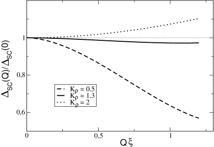
Figure 1: Superconducting gap (normalized to its $Q=0$ value) vs $Q\xi$.

The real-frequency expression of the gap is obtained by the analytic continuation $(\omega_{n})^{2}\rightarrow-(\omega+i\epsilon)^{2}$ in Eq. (9). For $|\omega|>\cal{M}$, the hypergeometric functions have branch cuts, leading to a nonzero imaginary part in $\Delta_{SC}(0,\omega)$ as can be seen on Fig. 2(b). Above the threshold, the gap function presents a singular behavior: $\Delta(0,\omega)\sim\Delta(0,0)(1-\frac{(\omega+i0)^{2}}{{\cal M}^{2}})^{-\frac{1}{2K_{\rho}}}$. The divergence at $\omega={\cal M}$ is in fact cut-off once $|\omega-{\cal M}|<1/L$ since we are really dealing with a system of finite size, so that $\Delta_{\rm SC}(q,\omega\rightarrow{\cal M})={\cal M}$. The full $\omega$-dependence of $\Delta_{\rm SC}$ plotted in Fig. 2(a) indeed reveals a strong singularity at $\omega={\cal M}$ increasingly pronounced as system size is increased.

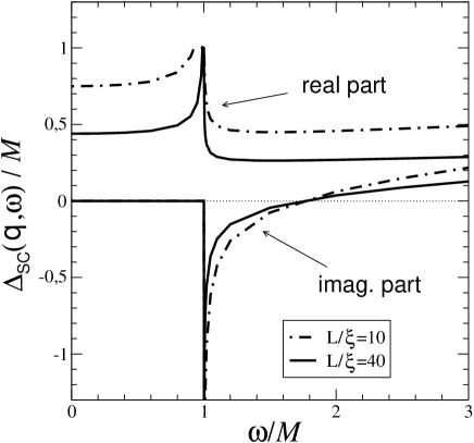
Figure 2: Real (a)) and imaginary (b) parts of the superconducting gap vs $\omega$ obtained by bosonization results for a 1D LE liquid (energies are in units of the spectral (solitonic) gap $\cal M$) for $K_{\rho}=1.3$ and $q=k_{F}$. Data for two lengths are shown.

In the absence of data for a single attractive Hubbard chain or a single $t-J$ chain, we compare our results to numerical calculations on the t-J ladder model at $1/8$-doping and $J=0.4$poilblanc_gap_2leg . The numerical calculations on $2\times 12$ ladder show that there are two spinon gaps, ${\cal M}(q_{y}=0)=0.08t$ and ${\cal M}(q_{y}=\pi)=0.12t$ such that $F(q_{y}=0,\pi)$, $G(q_{y}=0,\pi)$ and $\Delta(q_{y}=0,\pi)$ develop an imaginary part for $\omega>\Delta(q_{y})$. The comparison of these spinon gaps with the actual spin gap of a $2\times 24$ ladderCORE (defined as the gap between the lowest triplet excitation and the singlet ground state) gives $\Delta_{\sigma}(q_{y}=0)=0.11t\simeq 2{\cal M}(q_{y}=0)$ and $\Delta_{\sigma}(q_{y}=\pi)=0.17t\simeq{\cal M}(q_{y}=\pi)+{\cal M}(q_{y}=0)$. The discrepancies could result from a spinon-spinon attraction or from the overestimation of the spinon gaps in the $2\times 12$ ladder. It is also important to note that in poilblanc_gap_2leg , the correlation length is of the order of magnitude of the system size. We note that no sharp peak is present in the imaginary part at the threshold, in contrast to the prediction of (9), but the prediction of a rather constant behavior of $\Delta$ below the threshold is in agreement with (9).

A more detailed comparison between analytic and numerical result is possible. In the case of the ladder system, away from half-filling, the gapped modes is expected to present an approximate $SO(6)\sim SU(4)$ symmetryschulz_son ; ahn_paik . This allows a description of the gapped modes by the SO(6) Gross-Neveu (GN) modelgross_neveu and a form factor calculation of the superconducting gap $\Delta({\bf q},\omega_{n})$ along the lines of the present paperahn_paik . The novelty in the case of the $SO(6)$ GN model is that on top of the spinon excitations of mass ${\cal M}$ (known as kinks in the literature on the GN model), there are also massive fermion excitations (bound states) with a mass ${\cal M}\sqrt{2}$. This implies a second threshold in $\Delta({\bf q},\omega_{n})$ at the energy $\omega={\cal M}(1+\sqrt{2})$ besides the threshold at energy $\omega={\cal M}$. Whether this could be related to some higher energy features seen in numerics poilblanc_gap_2leg needs further clarifications. This will be discussed in more details in a separate publication.

In conclusion, we have computed the fluctuating SC gap of the LE chain. A simple form is obtained with a factorization into a power-law factor accounting for SC suppression due to quantum phase fluctuations multiplied by a function containing the dynamics of the pairing interaction. We point out some differences with the case of the 2-leg t-J ladder and suggest that the gapped sectors of the latter could be better described by the SO(6) GN model.

References

- (1) J. R. Schrieffer, in Theory of Superconductivity (Addison-Wesley, Reading, MA, 1964), Chap. 7.
- (2) D. Poilblanc and D. J. Scalapino, Phys. Rev. B 66, 052513 (2002).
- (3) D. Poilblanc, D. J. Scalapino and S. Capponi (unpublished).
- (4) E. Dagotto and T. M. Rice, Science 271, 618 (1996), and references therein.
- (5) H. J. Schulz, in Correlated fermions and transport in mesoscopic systems, edited by T. Martin, G. Montambaux, and J. Tran Thanh Van (Editions frontières, Gif sur Yvette, France, 1996), p. 81.
- (6) E. Dagotto, Rep. Prog. Phys. 62, 1525 (1999).
- (7) H. J. Schulz, in Mesoscopic quantum physics, Les Houches LXI, edited by E. Akkermans, G. Montambaux, J. L. Pichard, and J. Zinn-Justin (Elsevier, Amsterdam, 1995), p. 533.
- (8) For numerical studies see e.g. C. A. Hayward et al., Phys. Rev. Lett. 75, 926 (1995); D. Poilblanc, D.J. Scalapino, and W. Hanke, Phys. Rev. B 52, 6796 (1995).
- (9) H. J. Mikeska and H. Schmidt, J. Low Temp. Phys 2, 371 (1970).
- (10) N. D. Mermin and H. Wagner, Phys. Rev. Lett. 17, 1133 (1967).
- (11) J. Voit, Eur. Phys. J. B 5, 505 (1998).
- (12) A. M. Tsvelik and F. H. L. Essler, cond-mat/0205294 (unpublished).
- (13) A. Luther and V. J. Emery, Phys. Rev. Lett. 33, 589 (1974).
- (14) N. Andrei, in Low-Dimensional Quantum Field Theories For Condensed Matter Physicists, edited by S. Lundqvist, G. Morandi, and L. Yu (World Scientific, Singapore, 1993), and references therein.
- (15) M. Nakamura, K. Nomura, and A. Kitazawa, Phys. Rev. Lett. 79, 3214 (1997), cond-mat/9708204.
- (16) N. Andrei and J. H. Lowenstein, Phys. Rev. Lett. 43, 1698 (1979).
- (17) M. Karowski and P. Wiesz, Nucl. Phys. B 139, 455 (1978).
- (18) D. Controzzi, F. H. L. Essler, and A. M. Tsvelik, in New Theoretical approaches to strongly correlated systems, Vol. 23 of NATO Science Series II. Mathematics, Physics and Chemistry, edited by A. M. Tsvelik (Kluwer Academic Publishers, Dordrecht, 2001), p. 25.
- (19) F. H. Essler and V. E. Korepin, cond-mat/9808018 (unpublished).
- (20) S. Lukyanov and A. B. Zamolodchikov, Nucl. Phys. B 607, 437 (2001).
- (21) M. Abramowitz and I. Stegun, Handbook of mathematical functions (Dover, New York, 1972).
- (22) H. Schulz, cond-mat/9808167 (unpublished).
- (23) D. J. Gross and A. Neveu, Phys. Rev. D 10, 3235 (1974).
- (24) Data obtained using an approximate Contractor Renormalisation (CORE) method; see S. Capponi and D. Poilblanc, Phys. Rev. B 66, 180503 (2002) and references therein.
- (25) Numerical investigations of boundstates are given in D. Poilblanc, O. Chiappa, S. White and D. J. Scalapino, Phys. Rev. B 62, R14633 (2000).
- (26) A calculation of the spectral functions in the ladder using the SO(6) GN model has been reported in C. Ahn and E. Paik, J. Korean Phys. Soc. 39, 965 (2001).