Monte Carlo Study of Ordering and Domain Growth in a Class of fcc–Alloy Models

Abstract

Ordering processes in fcc–alloys with composition $A_{3}B$ (like Cu₃Au, Cu₃Pd, CoPt₃ etc.) are investigated by Monte Carlo simulation within a class of lattice models based on nearest–neighbor (NN) and second-neighbor (NNN) interactions. Using an atom–vacancy exchange algorithm, we study the growth of ordered domains following a temperature quench below the ordering spinodal. For zero NNN-interactions we observe an anomalously slow growth of the domain size $L(t)\sim t^{\alpha}$, where $\alpha\sim 1/4$ within our accessible timescales. With increasing NNN–interactions domain growth becomes faster and $\alpha$ gradually approaches the value 1/2 as predicted by the conventional Lifshitz–Allen–Cahn theory.

1 Introduction

Ordering transitions in real metallic alloys normally show kinetic properties which are substantially more complex than the standard Lifschitz–Allen–Cahn scenario in the case of a scalar, non–conserved order–parameter [1, 2]: i) The symmetry of the ordered phase can imply a multicomponent order–parameter and the appearance of several antiphase domains. ii) There may be different types of domain boundaries providing different forces for curvature–driven coarsening. iii) Coupling of non–conserved order–parameter components to the (conserved) alloy composition generally leads to compositional changes within domain boundaries. Domain growth hence is accompanied and slowed down by interdiffusion processes. iv) Depending on properties of the chemical interactions, vacancies may enrich in the domain boundaries and thus enhance the dynamics when atom–vacancy exchange is the prevailing migration mechanism [3, 4]. v) Quenching into a two–phase region in the temperature–concentration plane releases competing processes of ordering and spinodal decomposition, eventually accompanied by the appearance of transient phases. vi) Finally we mention effects caused by surfaces or imperfections, which break the lattice translational symmetry.

Despite a large body of literature [5], many questions in this area have remained open. Our aim here is to study some new qualitative aspects primarily in connection with the first two points listed above. For that purpose we consider fcc $A_{3}B$–type alloys (such as Cu₃Au, Cu₃Pd etc.) that display an ordered $L1_{2}$–structure. A class of models is considered which includes chemical interactions on the fcc–lattice up to second neighbors. Our main result will be to demonstrate a gradual changeover from an anomalously slow growth with an effective exponent $\alpha\sim 1/4$ to conventional growth, characterized by $\alpha=1/2$, when the second neighbor interactions are increased from zero. Results will be interpreted in terms of properties of low–energy or type–I domain walls, whose energy vanishes as the second–neighbor interactions are switched off.

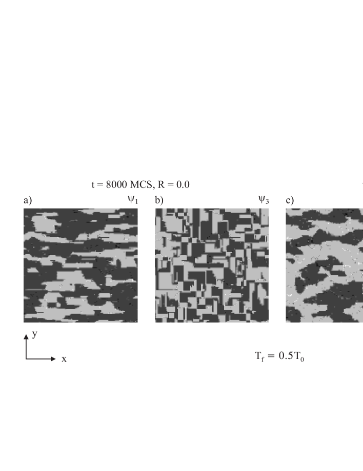
Figure 1: Comparison of domain patterns reflected by $\psi_{1}$ at $T=0.5\,T_{0}$ for a) $R=0$; $t=8\cdot 10^{3}$ MCS and c) $R=0.3$; $t=3\cdot 10^{2}$ MCS, while $\psi_{3}$–patterns are shown in b) and d) for the same parameters. From the figures type–I and type–II walls can clearly be distinguished.

2 Fcc–alloy model with vacancy–driven kinetics

Consider an fcc–lattice, where each site i can be occupied by an $A$-atom, a $B$-atom or a vacancy ($V$). Occupation numbers thus satisfy $c_{i}^{A}+c_{i}^{B}+c_{i}^{V}=1$. Their averages over all sites are chosen in accord with stoichiometric $A_{3}B$ alloys, $c^{A}=3c^{B}$. The average vacancy concentration $c^{V}\ll 1$ is taken small enough so that static properties are unaffected by the vacancies. For NN–sites $i$ and $j$ interactions are taken as in our previous work [6], $V_{ij}^{BB}=V^{BB}>0$; $V_{ij}^{AA}=V_{ij}^{AB}=-V^{BB}$. On the other hand, for NNN–sites $i$ and $j$ we assume $V_{ij}^{BB}=V^{AA}_{ij}=RV^{BB}$; $V_{ij}^{AB}=0$, with $0\leq R\leq 0.5$.

The above model displays a 4-fold degenerate ground state corresponding to the ideal $L1_{2}$–structure. This structure is described by a 4–component order parameter [7], $\Psi=(\psi_{0},\psi_{1},\psi_{2},\psi_{3})$, where $\psi_{0}$ refers to the $A/B$–concentration, while $\psi_{1}$, $\psi_{2}$ and $\psi_{3}$ describe a succession of $B$-rich and $B$–depleted atomic layers along the $x$–, $y$– and $z$–direction, respectively. Ordered domains are of the type $(\psi_{1},\psi_{2},\psi_{3})\propto(-1,1,1);(1,-1,1);(1,1,-1)$ and $(-1,-1-1)$. A sign–change of $\psi_{1}$ along the $x$–direction implies a high–energy type–II domain wall. Along the $y$– or $z$–direction a sign change of $\psi_{1}$ can be effected without braking nearest–neighbor bonds, and creates a low–energy type–I wall. Its energy solely results from NNN–interactions and therefore is zero if $R=0$.

In our Monte Carlo simulations we employ the atom–vacancy exchange algorithm. The ordering temperature $T_{0}$ and the temperature for spinodal ordering $T_{sp}$ are deduced from simulations as in [8]. At $R=0$ we have $k_{B}\,T_{0}=1.83\,V_{BB}/2$, while $T_{sp}\simeq 0.967\,T_{0}$. $T_{0}$ and $T_{sp}$ increase nearly linearly with $R$, such that $T_{0}(R)/T_{0}(0)\simeq 2.38$ and $T_{sp}(R)/T_{sp}(0)\simeq 2.43$ at $R=0.5$.

Typical domain patterns observed after a sudden quench from infinite temperature to a final temperature $T<T_{sp}$ are shown in Figs. 1a,b for $R=0$ and in Figs. 1c,d for $R=0.3$. Evolution times after the quench were chosen such that the typical domain sizes (see section 3) nearly agree in both cases. Apart from the much faster evolution in the case $R=0.3$ the most important observation is that type–I walls in Figs. 1a,b are flat and nearly perfect, whereas in Figs. 1c,d they show curvature and larger fluctuations. A connection of these different behaviors to kinetic properties will be discussed in section 3.

Using experimental tracer diffusion constants for calibration, our algorithm allows us to relate the Monte Carlo time to the physical timescale in kinetic processes. Details of this analysis, applied to Cu₃Au, are described in [6]. As an order–of–magnitude approximation we find that $1$ MCS roughly corresponds, for example, to $0.1s$ at $T=0.9\,T_{0}$ and $10^{7}s$ at $T=0.5\,T_{0}$. We come back to this point in section 3 when discussing different temporal regimes in domain coarsening processes.

Figure 2: Evolution of the excess energy $\Delta E(t)$ per lattice site for different temperatures $T$ and different NNN–interactions: a) $R=0$; b) $R=0.1$; c) $R=0.3$ and d) $R=0.5$. Dotted lines have slopes corresponding to $\alpha=1/4$ and $\alpha=1/2$.

3 Domain growth – results and discussion

For a quantitative analysis of the structure and growth of domains we introduce equal–time structure factors $S_{\alpha}(\vec{k},t)=\langle|\Psi_{\alpha}(\vec{k},t)|^{2}\rangle$. In view of the sign changes in the local order parameters $\psi_{\alpha}(\vec{r},t)$ across a wall, see section 2, it is clear that the linear combinations

$$S_{||}(k,t)=\frac{1}{3}\left(S_{1}(k,0,0,t)+S_{2}(0,k,0,t)+S_{3}(0,0,k,t)\right)$$ (1)

and

$$S_{\perp}(k,t)=\frac{1}{N_{k}}\sum_{q_{1}^{2}+q_{2}^{2}=k^{2}}\left(S_{1}(0,q_{1},q_{2},t)+S_{2}(q_{1},0,q_{2},t)+S_{3}(q_{1},q_{2},0,t)\right)$$ (2)

reflect the arrangement of type–II and type–I walls, respectively. In Eq. (2), $N_{k}$ denotes the number of pairs $(q_{1},q_{2})$ that fulfill $q_{1}^{2}+q_{2}^{2}=k^{2}$. Typical distances between walls of either type are determined by the first moments $k_{||}(t)$ and $k_{\perp}(t)$ of the structure factors (1) and (2). In addition we study the excess energy stored in the domain walls, $\Delta E(t)=E(t)-E(\infty)$, where $E(\infty)$ is the energy after complete equilibration.

Figure 3: Evolution of the first moment $k_{||}(t)$ of the structure factor $S_{||}(k,t)$ for different temperatures $T$ and different NNN–interactions: a) $R=0$; b) $R=0.1$; c) $R=0.3$ and d) $R=0.5$.

In the following we focus on $T<T_{sp}$. In Fig. 2a-d $\Delta E(t)$–data are presented for different $R$. At the highest temperature $T=0.9\,T_{0}$, which in all cases is slightly below $T_{sp}$, a shoulder as a remnant of an incubation period in the metastable regime is still visible, while a power–law–type decay of $\Delta E(t)$ prevails for deeper quenches. A similar behavior is found for $k_{||}(t)$, see Fig. 3 and also for $k_{\perp}(t)$ (not shown), which is always larger than $k_{||}(t)$. The important observation is that within the timescales of our simulations these power–laws change with $R$. As mentioned already, at $R=0$ where type–I walls have zero energy, an anomalously slow growth is found, that can be represented by an effective exponent $\alpha\simeq 1/4$ within an extended time window up to our largest computing times. Upon introducing small second–neighbor interactions with $R=0.1$ we observe a significantly faster growth. This becomes particularly evident by comparing the data for the lowest temperature $T=0.5\,T_{0}$ in Figs. 2a and 3a with those in Figs. 2b and 3b. The slope of these data corresponds to exponents still significantly smaller than 1/2. Further increase of $R$ to $R=0.3$ (Figs. 2c and 3c) yields exponents close to the “normal” behavior $\alpha=1/2$, pertaining here to $T\leq 0.7\,T_{0}$ and to a time regime starting even below $10^{2}$ MCS. No substantial change occurs when going to $R=0.5$, as shown in Figs. 2d and 3d. The steeper decay near $t\sim 10^{4}$ MCS can be traced back to finite size effects, as $k_{||}^{-1}$ becomes of the order of the size $L=128$ of the simulation cell. These findings support the conclusion that the extraordinary slow growth in the case of zero NNN–interactions ($R=0$) arises from the existence of zero–energy, curvatureless domain walls of type I, which are extremely stable. Within the time window considered, such behavior appears representative for a class of systems with $R$ small, where type–I walls have sufficiently small, but non–zero energy.

Clearly, our results especially for $R\leq 0.1$ do not allow us to draw any conclusion as to the exact asymptotics for quantities displayed in Figs. 2 and 3. However, from the discussion at the end of section 2 it appears that simulations up to $10^{4}$ MCS already exhaust the timescales relevant to experiments for quenches sufficiently below the spinodal.

From the discussion of Fig. 1 it is clear that structure factors $S_{\alpha}$ for a given $\alpha$ are affected by a 1–dimensional (1–d) array of type–II walls parallel to the $\alpha$–direction and a 2–d array of type–I walls perpendicular to it. Hence we expect the structure factors $S_{||}$ and $S_{\perp}$ to obey scaling laws for 1–d and 2–d systems, respectively [9]. This is verified in Fig. 4 showing master curves for $S_{||}$ and $S_{\perp}$ when scaled according to Porod’s law in one and two dimensions. This plot, applying to $R=0.5$, is very similar to analogous plots in [6] for $R=0$.

Figure 4: Structure factors $S_{||}(k,t)$ a) and $S_{\perp}(k,t)$ b) scaled according to Porod’s law in $d=1$ and $d=2$, respectively, at $T=0.5\,T_{0}$ for $R=0.5$.

References

- [1] I. M. Lifshitz, Sov. Phys. JETP 15, 939 (1962); J. Exp. Theor. Phys. (U.S.S.R) 42, 1354 (1962).
- [2] S. M. Allen and J. W. Cahn, Acta Metall. 27, 1085 (1979).
- [3] M. Porta, E. Vives, and T. Castan, Phys. Rev. B60, 3920 (1999)
- [4] C. Frontera, E. Vives, T. Castán, and A. Planes, Phys. Rev. B55, 212 (1997).
- [5] F. Ducastelle Order and Phase Stability in Alloys, F. R. De Boer, D. Pettifor (Eds.) North Holland (1991).
- [6] M. Kessler, W. Dieterich, and A. Majhofer, Phys. Rev. B, in press (2003).
- [7] Z.–W. Lai, Phys. Rev. B41, 9239 (1990).
- [8] M. Kessler, W. Dieterich, and A. Majhofer, Phys. Rev. B64, 125412-1 (2001).
- [9] A. J. Bray, Advances in Physics 43, 357 (1994).