Chapter 1 Introduction

If one is used to looking at chemical processes from an atomic point of view, then the field of chemical kinetics is very complicated. Kinetics is generally studied on meso- or macroscopic scales. Atomic scales are of the order of Ångstrøm and femtoseconds. Typical length scales in laboratory experiments vary between micrometers to centimeters, and typical time scales are often of the order of seconds or longer. This means that there many orders of difference in length and time between the individual reactions and the resulting kinetics.

The length gap is not always a problem. Many systems are homogeneous, and the kinetics of a macroscopic system can be reduced to the kinetics of a few reacting molecules. This is generally the case for reactions in the gas phase and in solutions. For reactions on the surface of a catalyst it is not clear when this is the case. It is certainly the case that in the overwhelming number of studies on the kinetics in heterogeneous catalysis it is implicitly assumed that the adsorbates are well-mixed, and that macroscopic rate equations can be used. These equations have the form

$${d\theta_{\rm A}\over dt} = -k_{\rm A}^{(1)}\theta_{\rm A}+\sum_{\rm B\neq A}k_{\rm B}^{(1)}\theta_{\rm B}$$

$$-2k_{\rm A}^{(2)}\theta_{\rm A}^{2}-\sum_{\rm B\neq A}k_{\rm AB}^{(2)}\theta_{\rm A}\theta_{\rm B}+\sum_{\rm B,C\neq A}k_{\rm BC}^{(2)}\theta_{\rm B}\theta_{\rm C}+\ldots$$

with $\theta_{\rm A}$ the so-called coverage of adsorbate A, which is the number of A’s per unit area of the surface on which the reactions take place. The terms stand for the reactions ${\rm A}\to\ldots$, ${\rm B}\to{\rm A}$, $2{\rm A}\to\ldots$, ${\rm A}+{\rm B}\to\ldots$, and ${\rm B}+{\rm C}\to{\rm A}$, respectively. The $k$’s are rate constants. If a position dependence $\theta=\theta({\bf r},t)$ is included we also need a diffusion term. The result is called a reaction-diffusion equation. Simulations of reactions on surfaces and detailed studies in surface science over the last few years have shown that the macroscopic rate equations are only rarely correct. Moreover, there are systems that show the formation of patterns with a characteristic length scale of micro- to centimeters. For such systems it is not clear at all what the relation is between the macroscopic kinetics and the individual reactions.

Even more of a problem is the time gap. The typical atomic time scale is given by the period of a molecular vibration. The fastest vibrations have a reciprocal wavelength of up to $4000\,\hbox{cm}^{-1}$, and a period of about $8.3\,$fs. Reactions in catalysis take place in seconds or more. It is important to be aware of the origin of these fifteen orders of magnitude difference. A reaction can be regarded as a movement of the system from one local minimum on a potential-energy surface to another. In such a move a so-called activation barrier has to be overcome. Most of the time the system moves around one local minimum. This movement is fast, in the order of femtoseconds, and corresponds to a superposition of all possible vibrations. Every time that the system moves in the direction of the activation barrier can be regarded as an attempt to react. The probability that the reaction actually succeeds can be estimated by calculating a Boltzmann factor that gives the relative probability of finding the system at a local minimum or on top of the activation barrier. This Boltzmann factor is given by $\exp[-E_{\rm bar}/RT]$, where $E_{\rm bar}$ is the height of the barrier, $R$ is the gas constant, and $T$ is the temperature. A barrier of $E_{\rm bar}=100\,$kJ/mol at room temperature gives a Boltzmann factor of about $10^{-18}$. Hence we see that the very large difference in time scales is due to the very small probability that the system overcomes activations barriers.

In Molecular Dynamics a reaction with a high activation barrier is called a rare event, and various techniques have been developed to get a reaction even when a standard simulation would never show it. These techniques, however, work for one reacting molecule or two molecules that react together, but not when one is interested in the combination of thousands or more reacting molecules that one has when studying kinetics. The purpose of this course is to show how one deals with such a collection of reacting molecules. It turns out that one has to sacrifices some of the detailed information that one has in Molecular Dynamics simulations. One can still work on atomic length scales, but one cannot work with the exact position of all atoms in a system. Instead one only specifies near which minimum of the potential-energy surface the system is. One does not work with the atomic time scale. Instead one has the reactions as elementary events: i.e., one specifies at which moment the system moves from one minimum of the potential-energy surface to another. Moreover, because one doesn’t know where the atoms are exactly and how they are moving, one cannot determine the times for the reactions exactly either. Instead one can only give probabilities for the times of the reactions. It turns out, however, that this information is more than sufficient for studying kinetics.

Chapter 2 A Stochastic Model for the Description of Surface Reaction Systems

2.1 The lattice gas

The size of the time step, and with this computational cost, in simulations of the motion of atoms and molecules is determined by the fast vibrations of chemical bonds.[1] Because the activation energies of chemical reactions are generally much higher than the thermal energies, chemical reactions take place on a time scale that is many orders of magnitude larger. If one wants to study the kinetics on surfaces, then one needs a method that does away with the fast motions.

The method that we present here does this by using the concept of sites. The forces working on an atom or a molecule that adsorbs on the catalyst force it to well-defined positions on the surface.[2, 3] These positions are called sites. They correspond to minima on the potential-energy surface for the adsorbate. Most of the time adsorbates stay very near these minima. Only when they diffuse from one site to another or during a reaction they will not be near a minima for a very short time. Instead of specifying the precise positions, orientations, and configurations of the adsorbates we will only specify for each sites its occupancy. A reaction and a diffusion from one site to another will be modeled as a sudden change in the occupancy of the sites. Because the elementary events are now the reactions and the diffusion, the time that a system can be simulated is no longer determined by fast motions of the adsorbates. By taking a slightly larger length scale, we can simulate a much longer time scale.

If the surface of the catalyst has two-dimensional translational symmetry, or when it can be modeled as such, the sites form a regular grid or a lattice. Our model is then a so-called lattice-gas model. This chapter shows how this model can be used to describe a large variety of problems in the kinetics of surface reactions.

2.1.1 Definitions

If the catalyst has two-dimensional translational symmetry then there are two vectors, ${\bf a}_{1}$ and ${\bf a}_{2}$, with the property that when the catalyst is translated over any of these vectors the result is indistinguishable from the situation before the translation. It is said that the system is invariant under translation over these vectors. The vectors ${\bf a}_{1}$ and ${\bf a}_{2}$ are called primitive vectors. In fact the catalyst is invariant under translational for any vector of the form

$${\bf x}=n_{1}{\bf a}_{1}+n_{2}{\bf a}_{2}$$ (2.1)

where $n_{1}$ and $n_{2}$ are integers. These vectors are the lattice vectors. The primitive vectors ${\bf a}_{1}$ and ${\bf a}_{2}$ are not uniquely defined. For example a (111) surface of a fcc metal is translationally invariant for ${\bf a}_{1}=a(1,0)$ and ${\bf a}_{2}=a(1/2,\sqrt{3}/2)$, where $a$ is the lattice spacing. But one can just as well choose ${\bf a}_{1}=a(1,0)$ and ${\bf a}_{2}=a(-1/2,\sqrt{3}/2)$. The area defined by

$${\bf x}=x_{1}{\bf a}_{1}+x_{2}{\bf a}_{2}$$ (2.2)

with $x_{1},x_{2}\in[0,1\rangle$ is called the unit cell. The whole system is retained by tiling the plane with the contents of a unit cell.

Expression (2.1) defines a simple lattice, Bravais lattice, or net. Simple lattices have just one lattice point, or grid point, per unit cell. It is also possible to have more than one lattice point per unit cell. The lattice is then given by all

$${\bf x}={\bf x}_{0}^{(i)}+n_{1}{\bf a}_{1}+n_{2}{\bf a}_{2}$$ (2.3)

with $i=0,1,\ldots,N_{\rm sub}-1$. Each ${\bf x}_{0}^{(i)}$ is a different vectors in the unit cell. The set ${\bf x}_{0}^{(i)}+n_{1}{\bf a}_{1}+n_{2}{\bf a}_{2}$ for a particular vector $i$ forms a sublattice, which is itself a simple lattice. There are $N_{\rm sub}$ sublattices, and they are all equivalent; they are only translated with respect to each other. (For more information on lattices see for example references [4] and [2]).

We assign a label to each lattice point. The lattice points correspond to the sites, and the labels specify properties of the sites. The most common property that one wants to describe with the label is the occupancy of the site. For example, the short-hand notation $(n_{1},n_{2}/s:{\rm A})$ can be interpreted as that the site at position ${\bf x}_{0}^{(s)}+n_{1}{\bf a}_{1}+n_{2}{\bf a}_{2}$ is occupied by a molecule A. The labels can also be used the specify reactions. A reaction is nothing but a change in the labels. An extension of the short-hand notation $(n_{1},n_{2}/s:{\rm A}\to{\rm B})$ indicates that during a reaction the occupancy of the site at ${\bf x}_{0}^{(s)}+n_{1}{\bf a}_{1}+n_{2}{\bf a}_{2}$ changes from A to B. If more than one site is involved in a reaction then the specification will consist of a set changes of the form $(n_{1},n_{2}/s:{\rm A}\to{\rm B})$.

2.1.2 Examples

Figure 2.1 shows a Pt(111) surface. CO prefers to adsorb on this surface at the top sites.[2] We can therefore model CO on this surface with a simple lattice with the lattice points corresponding to the top sites. We have ${\bf a}_{1}=a(1,0)$ and ${\bf a}_{2}=a(1/2,\sqrt{3}/2)$. As $N_{\rm sub}=1$ we choose ${\bf x}_{0}^{(0)}=(0,0)$ for simplicity. Each grid point has a label that we choose to be equal to CO or $*$. The former indicates that the site is occupied by a CO molecule, the latter that the site is vacant.

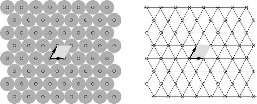
Figure 2.1: On the left is shown the top layer of a Pt(111) surface with the primitive vectors, the unit cell, and the top sites. On the right is shown the lattice formed by the top sites. The lines are guides for the eyes.

Desorption of CO from Pt(111) can be written as $(0,0:{\rm CO}\to*)$, where we have left out the index of the sublattice, because, as there is only one, it is clear on which sublattice the reaction takes place (see figure 2.2). Desorption on other sites can be obtained by translations over lattice vectors; i.e., $(0,0:{\rm CO}\to*)$ is representative for $(n_{1},n_{2}:{\rm CO}\to*)$ with $n_{1}$ and $n_{2}$ integers. Diffusion of CO can be modeled as hops from one site to a neighboring site. We can write that as $\{(0,0:{\rm CO}\to*),(1,0:*\to{\rm CO})\}$. Hops on other sites can again be obtained from these descriptions by translations over lattice vectors, but also by rotations that leave the surface is invariant.

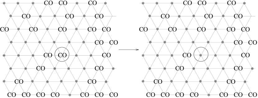
Figure 2.2: Change of labels for CO desorption from a Pt(111) surface. The encircled CO molecule on the left desorbs and the label becomes $*$ indicating a vacant site.

At high coverages the repulsion between the CO molecules forces some of them to bridge sites.[5] Figure 2.3 shows the new lattice. We have now for sublattices with ${\bf x}_{0}^{(0)}=(0,0)$, ${\bf x}_{0}^{(1)}=(1/2,0)$, ${\bf x}_{0}^{(2)}=(1/4,\sqrt{3}/4)$, ${\bf x}_{0}^{(3)}=(3/4,\sqrt{3}/4)$. The first one is for the top sites. The others are for the three sublattices of bridge sites. The figure shows that the lattice looks like a simple lattice. Indeed we can regard as such, but only when we need not distinguish between top and bridge sites.

Figure 2.3: On the left is shown the top layer of a Pt(111) surface with the primitive vectors, the unit cell, and the top and bridge sites. On the right is shown the lattice formed by the top and bridge sites sites. The lines are guides for the eyes.

NO on Rh(111) forms a $(2\times 2)$-3NO structure in which equal numbers of NO molecules occupy top, fcc hollow, and hcp hollow sites.[6, 7] Figure 2.4 shows the sites that are involved and the corresponding lattice. We now have three sublattices with ${\bf x}_{0}^{(0)}=(0,0)$ (top sites), ${\bf x}_{0}^{(1)}=(1/2,\sqrt{3}/6)$ (fcc hollow sites), and ${\bf x}_{0}^{(2)}=(1,\sqrt{3}/3)$ (hcp hollow sites). This is similar to the case with high CO coverage on Pt(111). $(0,0/0:{\rm NO})$ indicates that there is an NO molecule at the top site $(0,0)$, and $(0,0/1:*)$ indicates that the fcc hollow site at $(1/2,\sqrt{3}/6)$ is vacant.

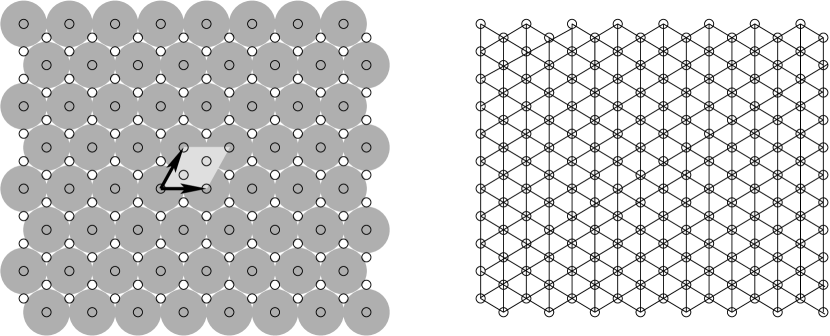
Figure 2.4: On the left is shown the top layer of a Rh(111) surface with the primitive vectors, the unit cell, and the top and hollow sites. On the right is shown the lattice formed by the top and hollow sites sites. The lines are guides for the eyes.

Note that also in this case the lattice resembles a simple lattice with ${\bf a}_{1}=a(1/2,\sqrt{3}/6)$ and ${\bf a}_{2}=a(\sqrt{3}/3,0)$. It is indeed also possible to model the system with this simple lattice, but one should note that then the difference between the top and hollow sites is ignored. It is possible to use the simple lattice and at the same time retaining the difference between the sites. The trick is to use the labels not just for the occupancy, but also for indicating the type of site. So instead of labels NO and $*$ indicating the occupancy, we use NOt, NOf, NOh, $*$t, $*$f, and $*$h. The last letter indicates the type of site (t stands for top, f for fcc hollow, and h for hcp hollow) and the rest for the occupancy. Instead of $(0,0/0:{\rm NO})$ and $(0,0/1:*)$ we have $(0,0:{\rm NOt})$ and $(1,0:*{\rm f})$, respectively. It depends very much on the reaction which way of describing the system is more convenient and computationally more efficient.

Using the label to specify other properties of the site than its occupancy can be a very powerful tool. Figure 2.5 shows how to model a step.[8, 9] If the terraces are small then it might also be possible to work with a unit cell spanning the width of a terrace, but when the terraces become large this will be inconvenient as there will be many sublattices.

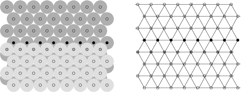
Figure 2.5: A Ru(0001) surface with a step and the top sites on the left. On the right is shown the lattice. The open circles are top sites on the terraces. The small black circles are top sites at the bottom of the step, and the small dark grey circles are top sites at the top of the step. The lines are guides for the eyes.

Site properties like the sublattice of which the site is part of and if it is a step site or not are static properties. The occupancy of a site is a dynamic property. There are also other properties of sites that are dynamic. Bare Pt(100) reconstructs into a quasi-hexagonal structure.[10] CO oxidation on Pt(100) is substantially influenced by this reconstruction because oxygen adsorbs much less readily on the reconstructed surfaces than on the unreconstructed one. This can lead to oscillation, chaos, and pattern formation.[10, 11] It is possible to model the effect of the reconstruction on the CO oxidation by using a label that specifies whether the surface is locally reconstructed or not.[12, 13, 14]

2.1.3 Shortcomings

The lattice-gas model is simple yet very powerful, as it allows us to model a large variety of systems and phenomena. Yet not everything can be modeled with it. Let’s take again CO oxidation on Pt(100). As stated above this system shows reconstruction which can be modeled with a label indicating that the surface is reconstructed or not. This way of modeling has shown to be very successful,[12, 13, 14] but it does neglect some aspects of the reconstruction. The reconstructed and the unreconstructed surface have very different unit cells, and the adsorption sites are also different.[15, 16] In fact, the unit cell of the reconstructed surface is very large, and there are a large number of adsorption sites with slightly different properties. These aspects have been neglected in the kinetic simulations so far. As these simulations have been quite successful, it seems that these aspects are not very relevant in this case, but that need not be always be the case. Catalytic partial oxidation (CPO) takes place at high temperature at which the surface is so dynamic that all translational symmetry is lost. In this case using a lattice to model the kinetics seems inappropriate.

The example of CO on Pt(111) has shown that at high coverage the position at which the molecules adsorb change. The reason for this is that these positions are not only determined by the interactions between the adsorbates and the substrate, but also by the interactions between the adsorbates themselves. At low coverages the former dominate, but at high coverages the latter may be more important. This may lead to adlayer structures that are incommensurate with the substrate.[2] Examples are formed by the nobles gases. These are weakly physisorbed, whereas at high coverages the packing onto the substrate is determined by the steric repulsion between them. At low and high coverages different lattices are needed to describe the positions of the adsorbates, but a single lattice describing both the low and the high coverage sites is not possible. Simulations in which the coverages change from low to high coverage and/or vice versa then cannot be based on a lattice-gas model.

2.2 The Master Equation

2.2.1 Definition

Our treatment of Monte Carlo simulations of surface reactions differs in one very fundamental aspect from that of other authors; the derivation of the algorithms and a large part of the interpretation of the results of the simulations are based on a Master Equation

$${dP_{\alpha}\over dt}=\sum_{\beta}\left[W_{\alpha\beta}P_{\beta}-W_{\beta\alpha}P_{\alpha}\right].$$ (2.4)

In this equation $t$ is time, $\alpha$ and $\beta$ are configurations of the adlayer, $P_{\alpha}$ and $P_{\beta}$ are their probabilities, and $W_{\alpha\beta}$ and $W_{\beta\alpha}$ are so-called transition probabilities per unit time that specify the rate with which the adlayer changes due to reactions. The Master Equation is a loss-gain equation. The first term on the right stands for increases in $P_{\alpha}$ because of reactions that change other configurations into $\alpha$. The second term stands for decreases because of reactions in $\alpha$. From

$${d\over dt}\sum_{\alpha}P_{\alpha}=\sum_{\alpha}{dP_{\alpha}\over dt}=\sum_{\alpha\beta}\left[W_{\alpha\beta}P_{\beta}-W_{\beta\alpha}P_{\alpha}\right]=0$$ (2.5)

we see that the total probability is conserved. (The last equality can be seen by swapping the summation indices in one of the terms.)

The Master Equation can be derived from first principles as will be shown below, and hence forms a solid basis for all subsequent work. There are other advantages as well. First, the derivation of the Master Equation yields expressions for the transition probabilities that can be computed with quantum chemical methods.[17] This makes ab-initio kinetics for catalytic processes possible. Second, there are many different algorithms for Monte Carlo simulations. Those that are derived from the Master Equation all give necessarily results that are statistically identical. Those that cannot be derived from the Master Equation conflict with first principles and should be discarded. Third, Monte Carlo is a way to solve the Master Equation, but it is not the only one. The Master Equation can, for example, be used to derive the normal macroscopic rate equation (see below). In general, it forms a good basis to compare different theories of kinetic quantitatively, and also to compare these theories with simulations.

2.2.2 Derivation

The Master Equation can be derived by looking at the surface and its adsorbates in phase space. This is, of course, a classical mechanics concept, and one might wonder if it is correct to look at the reactions on an atomic scale and use classical mechanics. The situation here is the same as for the derivation of the rate equations for gas phase reactions. The usual derivations there also use classical mechanics.[18, 19, 20, 21, 22] Although it is possible to give a completely quantum mechanical derivation formalism,[23, 24, 25, 26] the mathematical complexity hides much of the important parts of the chemistry. Besides, it is possible to replace the classical expressions that we will get by semi-quantum mechanical ones, in exactly the same way as for gas phase reactions.

A point in phase space completely specifies the positions and momenta of all atoms in the system. In Molecular Dynamics simulations one uses these positions and momenta at some starting point to compute them at later times. One thus obtains a trajectory of the system in phase space. We are not interested in that amount of detail, however. In fact as was stated before too much detail is detrimental if one is interested in simulating many reactions. The time interval that one can simulate a system using Molecular Dynamics is typically of the order of nanoseconds. Reactions in catalysis have a characteristic time that is many orders of magnitude longer. To overcome this large difference we need a method that removes the fast processes (vibrations) that determine the time scale of Molecular Dynamics, and leaves us with the slow processes (reactions). This method looks as follows.

Instead of the precise position of each atom, we only want to know how the different adsorbates are distributed over the sites of a surface. So our physical model is a lattice. Each lattice point corresponds to one site, and has a label that specifies which adsorbate is adsorbed. (A vacant site is simply a special label.) A particular distribution of the adsorbates over the sites, or, what is the same, a particular labeling of the grid points, we call a configuration. As each point in phase space is a precise specification of the position of each atom, we also know which adsorbates are at which sites; i.e., we know the corresponding configuration. Different points in phase space may, however, correspond to the same configuration, which differ only in slight variations of the positions of the atoms. This means that we can partition phase space in many region, each of which corresponds to one configuration. Reactions are then nothing but motion of the system in phase space from one region to another.

Because it is not possible to reproduce an experiment with exactly the same configuration, we are not only not interested in the precise position of the atoms, we are not even interested in specific configurations, but only in characteristic ones. Although there may be differences on a microscopic scale, the behavior of a system on a macroscopic, and often also on a mesoscopic, scale will be the same. So we do not look at individual trajectories in phase space, but we average over all possible trajectories. This means that we work with a phase space density $\rho$ and a probability $P_{\alpha}$ of finding the system in configuration $\alpha$. These are related via

$$P_{\alpha}(t)=\int_{R_{\alpha}}\!\!{d{\bf q}\,d{\bf p}\over h^{D}}\,\rho({\bf q},{\bf p},t),$$ (2.6)

where ${\bf q}$ stands for all coordinates, ${\bf p}$ stands for all momenta, $h$ is Planck’s constant, $D$ is the number of degrees of freedom, and the integration is over the region $R_{\alpha}$ in phase space that corresponds to configuration $\alpha$ (see figure 2.6). The denominator $h^{D}$ is not needed for a purely classical description of the kinetics. However, it makes the transition from a classical to a quantum mechanical description easier.[27]

Figure 2.6: Schematic drawing of the partitioning of configuration space into regions $R$, each of which corresponds to some particular configuration of the adlayer. The reaction that changes $\alpha$ into $\beta$ corresponds to a flow from $R_{\alpha}$ to $R_{\beta}$. The transition probability $W_{\beta\alpha}$ for this reaction equals the flux through the surface $S_{\beta\alpha}$, separating $R_{\alpha}$ from $R_{\beta}$, divided by the probability to find the system in $R_{\alpha}$.

The Master Equation tells us how these probabilities $P_{\alpha}$ change in time. Differentiating equation (2.6) yields

$${dP_{\alpha}\over dt}=\int_{R_{\alpha}}\!\!{d{\bf q}\,d{\bf p}\over h^{D}}\,{\partial\rho\over\partial t}({\bf q},{\bf p},t).$$ (2.7)

This can be transformed using the Liouville-equation[28]

$${\partial\rho\over\partial t}=-\sum_{i=1}^{D}\left[{\partial\rho\over\partial q_{i}}{\partial H\over\partial p_{i}}-{\partial\rho\over\partial p_{i}}{\partial H\over\partial q_{i}}\right]$$ (2.8)

into

$${dP_{\alpha}\over dt}=\int_{R_{\alpha}}\!\!{d{\bf q}\,d{\bf p}\over h^{D}}\,\sum_{i=1}^{D}\left[{\partial\rho\over\partial p_{i}}{\partial H\over\partial q_{i}}-{\partial\rho\over\partial q_{i}}{\partial H\over\partial p_{i}}\right],$$ (2.9)

where $H$ is the system’s classical Hamiltonian. To simplify the mathematics, we will assume that the coordinates are Cartesian and the Hamiltonian has the usual form

$$H=\sum_{i=1}^{D}{p_{i}^{2}\over 2m_{i}}+V({\bf q}),$$ (2.10)

where $m_{i}$ is the mass corresponding to coordinate $i$. We also assume that the area $R_{\alpha}$ is defined by coordinates only, and that the limits of integration for the momenta are $\pm\infty$. Although these assumptions are hardly restrictive, we would like to mention reference[29] for a more general derivation. The assumptions allow us to go from phase space to configuration space. (Not to be confused with the configurations of the Master Equation.) The first term of equation (2.9) now becomes

$$\int_{R_{\alpha}}\!\!{d{\bf q}\,d{\bf p}\over h^{D}}\,\sum_{i=1}^{D}{\partial\rho\over\partial p_{i}}{\partial H\over\partial q_{i}} =\sum_{i=1}^{D}\int_{R_{\alpha}}\!\!d{\bf q}\,{\partial V\over\partial q_{i}}\int_{-\infty}^{\infty}\!{d{\bf p}\over h^{D}}\,{\partial\rho\over\partial p_{i}}$$

$$=\sum_{i=1}^{D}\int_{R_{\alpha}}\!\!d{\bf q}\,{\partial V\over\partial q_{i}}\int_{-\infty}^{\infty}\!\!{dp_{1}\ldots dp_{i-1}dp_{i+1}\ldots dp_{D}\over h^{D}}$$

$$\qquad\times\big{[}\rho(p_{i}=\infty)-\rho(p_{i}=-\infty)\big{]}=0,$$

because $\rho$ has to go to zero for any of its variables going to $\pm\infty$ to be integrable. The second term becomes

$$-\int_{R_{\alpha}}\!\!{d{\bf q}\,d{\bf p}\over h^{D}}\,\sum_{i=1}^{D}{\partial\rho\over\partial q_{i}}{\partial H\over\partial p_{i}}=-\int_{R_{\alpha}}\!\!{d{\bf q}\,d{\bf p}\over h^{D}}\,\sum_{i=1}^{D}{\partial\over\partial q_{i}}\left({p_{i}\over m_{i}}\rho\right).$$ (2.12)

This particular form suggest using the divergence theorem for the integration over the coordinates.[30] The final result is then

$${dP_{\alpha}\over dt}=-\int_{S_{\alpha}}\!\!dS\int_{-\infty}^{\infty}\!{d{\bf p}\over h^{D}}\,\sum_{i=1}^{D}n_{i}{p_{i}\over m_{i}}\rho,$$ (2.13)

where the first integration is a surface integral over the surface of $R_{\alpha}$, and $n_{i}$ are the components of the outward pointing normal of that surface. Both the area $R_{\alpha}$ and the surface $S_{\alpha}$ are now regarded as parts of the configuration space of the system. As $p_{i}/m_{i}=\dot{q}_{i}$, we see that the summation in the last expression is the flux through $S_{\alpha}$ in the direction of the outward pointing normal (see figure 2.6).

The final step is now to decompose this flux in two ways. First, we split the surface $S_{\alpha}$ into sections $S_{\alpha}=\cup_{\beta}S_{\beta\alpha}$, where $S_{\beta\alpha}$ is the surface separating $R_{\alpha}$ from $R_{\beta}$. Second, we distinguish between an outward flux, $\sum_{i}n_{i}p_{i}/m_{i}>0$, and an inward flux, $\sum_{i}n_{i}p_{i}/m_{i}<0$. Equation (2.13) can then be rewritten as

$${dP_{\alpha}\over dt}= \sum_{\beta}\int_{S_{\alpha\beta}}\!\!dS\,\int_{-\infty}^{\infty}\!{d{\bf p}\over h^{D}}\,\left(\sum_{i=1}^{D}n_{i}{p_{i}\over m_{i}}\right)\Theta\left(\sum_{i=1}^{D}n_{i}{p_{i}\over m_{i}}\right)\rho$$ (2.14)

$$- \sum_{\beta}\int_{S_{\beta\alpha}}\!\!dS\,\int_{-\infty}^{\infty}\!{d{\bf p}\over h^{D}}\,\left(\sum_{i=1}^{D}n_{i}{p_{i}\over m_{i}}\right)\Theta\left(\sum_{i=1}^{D}n_{i}{p_{i}\over m_{i}}\right)\rho,$$

where in the first term $S_{\alpha\beta}$ ($=S_{\beta\alpha}$) is regarded as part of the surface of $R_{\beta}$, and the $n_{i}$ are components of the outward pointing normal of $R_{\beta}$. The function $\Theta$ is the Heaviside step function.[31] Equation (2.14) can be cast in the form of the Master Equation

$${dP_{\alpha}\over dt}=\sum_{\beta}\left[W_{\alpha\beta}P_{\beta}-W_{\beta\alpha}P_{\alpha}\right],$$ (2.15)

if we define the transition probabilities as

$$W_{\alpha\beta}=\left[\int_{S_{\alpha\beta}}\!\!dS\,\int_{-\infty}^{\infty}\!{d{\bf p}\over h^{D}}\,\left(\sum_{i=1}^{D}n_{i}{p_{i}\over m_{i}}\right)\Theta\left(\sum_{i=1}^{D}n_{i}{p_{i}\over m_{i}}\right)\rho\right]/\left[\int_{R_{\alpha}}\!\!d{\bf q}\,\int_{-\infty}^{\infty}\!{d{\bf p}\over h^{D}}\,\rho\right].$$ (2.16)

The expression for the transition probabilities can be cast in a more familiar form by using a few additional assumptions. We assume that $\rho$ can locally be approximated by a Boltzmann-distribution

$$\rho=N\exp\left[-{H\over k_{B}T}\right],$$ (2.17)

where $T$ is the temperature, $k_{B}$ is the Boltzmann-constant, and $N$ is a normalizing constant. We also assume that we can define $S_{\alpha\beta}$ and the coordinates in such a way that $n_{i}=0$, except for one coordinate $i$, called the reaction coordinate, for which $n_{i}=1$. The integral of the momentum corresponding to the reaction coordinate can then be done and the result is

$$W_{\alpha\beta}={k_{B}T\over h}{Q^{\ddagger}\over Q},$$ (2.18)

with

$$Q^{\ddagger} \equiv\int_{S_{\alpha\beta}}\!\!dS\,\int_{-\infty}^{\infty}\!{dp_{1}\ldots dp_{i-1}dp_{i+1}\ldots dp_{D}\over h^{D-1}}\exp\left[-{H\over k_{B}T}\right],$$ (2.19)

$$Q \equiv\int_{R_{\alpha}}\!\!d{\bf q}\,\int_{-\infty}^{\infty}\!{d{\bf p}\over h^{D}}\,\exp\left[-{H\over k_{B}T}\right].$$ (2.20)

We see that this is an expression that is formally identical to the Transition-State Theory (TST) expression for rate constants.[32] There are differences in the definition of the partition functions $Q$ and $Q^{\ddagger}$, but even these can be neglected as will be shown in chapter 3.

2.3 Working without a lattice

Although the use of a lattice is very important in the theory above, one should realize that it is really not needed from a theoretical point of view. No reference was made to a lattice in the derivation of the Master Equation, and indeed one can use the Master Equation also for reactive systems that do no have translational or any other kind of symmetry.

The idea is to look at the potential-energy surface (PES) of a system,[33] and associate each “configuration” $\alpha$ with a minimum of the PES. The region $R_{\alpha}$ consists of the points in phase space around the minimum (see figure 2.7). (As before the momenta can have any value.) The precise position of the surfaces $S_{\beta\alpha}$ are hard to determine. In Variational Transition-State Theory (VTST) they are chosen to minimize the flux,[18, 19, 20, 21, 22] but a more pragmatic approach would be to put $S_{\beta\alpha}$ at the saddle point of the PES that separates minimum $\alpha$ from $\beta$. The derivation in section 2.2.2 does not change, and we get a Master Equation describing processes/reactions corresponding to transitions between the minima of the PES. Again the fast motions in the system have been removed.

Figure 2.7: A potential-energy surface and the regions $R_{\alpha}$ around the minima. The lighter areas and the black contour lines depict lower values. The darker areas and the white contour lines depict the higher values. The fat dark lines indicate the boundaries $S_{\beta\alpha}$.

The advantage of a system with translation symmetry has to do with the number of different transition probabilities $W$. For the general case based on minima of the PES there is a different transition probability for each transition. For reactions on a surface the situation is simpler, because the same reaction occurring at different sites corresponds to different configuration changes but has the same transition probability.

Chapter 3 How to Get the Transition Probabilities?

The Master Equation is only useful if one knows the transition probabilities. There are basically two ways to get them. One way is to calculation them. The other is to derive them from experimental data.

3.1 Quantum chemical calculations of transition probabilities

There are three difference between expressions (2.19) and (2.20) for the partition function and those of TST.[32] The first is the absence of an exponential factor of the form $\exp(-E_{\rm bar}/k_{\rm B}T)$, the second is the boundaries of the integrations, and the third is the absence of a reference to a transition state. We deal with the boundaries first. Very often these can simply be removed. Define ${\bf q}^{({\rm min})}$ as the point in $R_{\alpha}$ at which $V$ is minimal, and approximate $V$ in $R_{\alpha}$ by

$$V_{\rm harm}({\bf q})=V({\bf q}^{({\rm min})})+{1\over 2}\sum_{i,j}(q_{i}-q_{i}^{({\rm min})}){\partial^{2}V\over\partial q_{i}\partial q_{j}}({\bf q}^{({\rm min})})(q_{j}-q_{j}^{({\rm min})}).$$ (3.1)

This is the harmonic approximation. A very common situation is the following. $V_{\rm harm}$ differs from $V$ only appreciably where $V-V({\bf q}^{({\rm min})})$ is large with respect to the thermal energy $k_{\rm B}T$. Because of the Boltzmann-factor in the integrals we can replace $V$ by $V_{\rm harm}$ in the integrals. The integration over $R_{\alpha}$ can then also be extended to infinity. The reason for this is that, in the region that has been added to the integral, the Boltzmann-factor with $V_{\rm harm}$ is so small that the added part is negligible. $Q$ thus becomes the normal expression for the classical partition function.

Note that we do not really need to make the harmonic approximation. Anharmonicities can be included. Instead of $V_{\rm harm}$ we can use any approximation to $V$ that is accurate at ${\bf q}$ unless $V({\bf q}-V({\bf q}^{({\rm min})})\gg k_{\rm B}T$, and the approximation should give negligible new contributions to the integrals when the boundaries are extended beyond $R_{\alpha}$.

For $Q^{\ddagger}$ we can draw the same conclusion. We restrict ourselves to $S_{\alpha\beta}$ and its extension defined by the coordinates used, and ${\bf q}^{({\rm min})}$ is the point on $S_{\alpha\beta}$ where $V$ is minimal. The rest of the reasoning is then the same as for $Q$. This also explains another difference with TST. The exponential factor is obtained by taking the $V({\bf q}^{({\rm min})})$ out off the integrals for $Q$ and $Q^{\ddagger}$. This immediately gives the exponential factor with $E_{\rm bar}$ equal to the difference between the minima of $V$ on $S_{\alpha\beta}$ and in $R_{\alpha}$.

There are two corrections to equation (2.16) that one might want to make. The first has to do with dynamical factors;[34, 35] i.e., trajectories leave $R_{\alpha}$, cross the surface $S_{\beta\alpha}$, but then immediately return to $R_{\alpha}$. Such a trajectory contributes to the transition probability $W_{\beta\alpha}$, but is not really a reaction. We can correct for this as in Variational Transition-State Theory (VTST) by shifting $S_{\beta\alpha}$ along the surface normals.[21, 22] This is related to the absence of any reference to any transition state so far. Indeed, if the $S_{\beta\alpha}$ can be chosen more or less arbitrarily provided the expression for $Q^{\ddagger}$ is corrected for the dynamical factors. Using the VTST approach $S_{\beta\alpha}$ will be well-defined. It turns out that with VTST the transition state (i.e., the saddle point between the minima in $R_{\alpha}$ and $R_{\beta}$) is generally very close to $S_{\beta\alpha}$, and taking $S_{\beta\alpha}$ so that it contains the transition state is often a very good approximation.[21, 22]

The second correction is for some quantum effects. Equation (2.18) indicates one way to include them. We can simply replace the classical partition functions by their quantum mechanical counterparts. (It is possible, of course, to do the integrals over the momenta in equations (2.19) and (2.20). The reason why we did not do that was to retain the correspondence between classical and quantum partition functions.) This does not correct for tunneling and interference effects, however. Inaccuracies due to tunneling, interference, and dynamic effects are not specific for the transition probabilities of the Master Equation. TST expressions have them too. As these effects are often small, this means that in practice one can use TST expressions to calculate the the transition probabilities of the Master Equation using quantum chemical methods in the same way as one calculates rate constants provided that the partition functions get the dominant contribution from a region in the integration range surrounding a minimum.

In the harmonic approximation we can write $Q$ as

$$Q=e^{-V_{\rm min}/k_{\rm B}T}\prod_{i}q_{v}(\omega_{i})$$ (3.2)

with $V_{\rm min}$ the minimum of the potential energy in $R_{\alpha}$. The vibrational partition function $q_{v}$ is given by

$$q_{v}(\omega)={k_{\rm B}T\over\hbar\omega}$$ (3.3)

classically, or

$$q_{v}(\omega)={e^{{1\over 2}\hbar\omega/k_{\rm B}T}\over 1-e^{\hbar\omega/k_{\rm B}T}}$$ (3.4)

quantum mechanically.[27, 28] The frequencies $\omega_{i}$ are the normal mode frequencies.[36, 37] Similarly we find for $Q_{\ddagger}$

$$Q^{\ddagger}=e^{-V_{\rm min}^{\prime}/k_{\rm B}T}\prod_{j}q_{v}(\omega_{j}^{\prime})$$ (3.5)

with $V_{\rm min}^{\prime}$ the minimum of the potential energy on $S_{\beta\alpha}$ and $\omega_{j}^{\prime}$ the non-imaginary normal mode frequencies at the transition state. Combining these results yields

$$W_{\beta\alpha}={k_{\rm B}T\over h}{\prod_{j}q_{v}(\omega_{j}^{\prime})\over\prod_{i}q_{v}(\omega_{i})}e^{-E_{\rm bar}/k_{\rm B}T}$$ (3.6)

with $E_{\rm bar}=V_{\rm min}^{\prime}-V_{\rm min}$.

It is very interesting to look in more detail at the case when it is not correct to extend the boundaries of the integrals. When the substrate has a closed-packed structure the potential-energy surface may be quite flat parallel to the surface. If that is the case there may be substantial contributions to the partition function up to the boundaries of the integrals. It is then not possible to apply the reasoning above. We will look at two examples; both dealing with simple desorption of an atom. In the first example the potential is completely flat parallel to the surface for all distances of the atom to the surface. In the second example the potential only becomes flat at the transition state.

Because dealing with a phase space of many atoms is inconvenient, we restrict ourselves to just one atom on the surface and calculate the transition state for desorption for that single atom. This is the usual approach; try to minimize the number of particles. The step to many atoms on the surface is made by assuming that the transition probability is independent on the number of atoms. This is correct if there are no lateral interactions, as we are assuming here. The case with lateral interactions will be discussed later.

Figure 3.1 show regions in phase space corresponding to an atom adsorbed on different sites. Crossing the upper horizontal plane bounding a region constitutes a desorption. Crossing one of the vertical planes bounding a region constitutes a diffusion to another site. The integrals of each momentum in the expression for the partition functions $Q$ and $Q^{\ddagger}$ become

$$\int_{-\infty}^{\infty}\!\!{dp\over h}\exp\left[-{p^{2}\over 2mk_{\rm B}T}\right]={1\over h}\sqrt{2\pi mk_{\rm B}T}.$$ (3.7)

The integrals of the coordinates for $Q^{\ddagger}$ become

$$\int_{S_{\alpha\beta}}\!\!dS\exp\left[-{V\over k_{\rm B}T}\right]=A_{\rm site}\exp\left[-{V(z_{\rm TS})\over k_{\rm B}T}\right],$$ (3.8)

where $z_{\rm TS}$ is the value of the coordinate perpendicular to the surface at the transition state for desorption, and $A_{\rm site}$ is the area of the horizontal boundary plane of a region or the area of a single site.

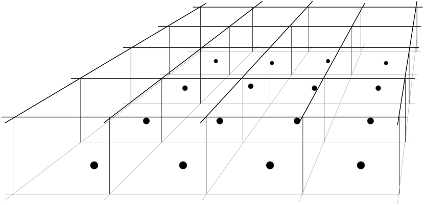
Figure 3.1: The phase space (or rather the configuration space, as the momenta are not shown) of a single atom. The lattice indicates the adsorption site and the bounded regions are parts of phase space corresponding to the atom being adsorbed on particular sites. The upper horizontal boundary plane contains the transition state for desorption. The lower horizontal plane represents the surface.

The integrals of the coordinates for $Q$ differ between our two examples. If the potential has a well-defined minimum near the adsorption site, then we can use the harmonic approximation (this is our second example).

$$V_{\rm harm} = V(x^{({\rm min})},y^{({\rm min})},z^{({\rm min})})$$

$$+ {1\over 2}m\omega_{\parallel}^{2}(x-x^{({\rm min})})^{2}+{1\over 2}m\omega_{\parallel}^{2}(y-y^{({\rm min})})^{2}+{1\over 2}m\omega_{\perp}^{2}(z-z^{({\rm min})})^{2}.$$

The integrals become

$$\int_{R}\!\!d{\bf q}\exp\left[-{V\over k_{\rm B}T}\right]={1\over\omega_{\parallel}^{2}\omega_{\perp}}\left({2\pi k_{\rm B}T\over m}\right)^{3/2}\exp\left[-{V(x^{({\rm min})},y^{({\rm min})},z^{({\rm min})})\over k_{\rm B}T}\right].$$ (3.10)

If the potential is flat parallel to the surface (this is our first example), then we can use the harmonic approximation only perpendicular to the surface. We get the same expression as above but with $\omega_{\parallel}=0$. The integrals now become

$$\int_{R}\!\!d{\bf q}\exp\left[-{V\over k_{\rm B}T}\right]=A_{\rm site}{1\over\omega_{\perp}}\left({2\pi k_{\rm B}T\over m}\right)^{1/2}\exp\left[-{V(x^{({\rm min})},y^{({\rm min})},z^{({\rm min})})\over k_{\rm B}T}\right].$$ (3.11)

All results can now be combined. For $Q^{\ddagger}$ the result is

$$Q^{\ddagger}=q_{f}^{2}\exp\left[-{V(z_{\rm TS})\over k_{\rm B}T}\right]$$ (3.12)

with

$$q_{f}\equiv{1\over h}\sqrt{2\pi A_{\rm site}mk_{\rm B}T},$$ (3.13)

which is the partition functions for one degree of freedom of a free particle. For the first example the partition function $Q$ becomes

$$Q=q_{f}^{2}q_{v}(\omega_{\perp})\exp\left[-{V(x^{({\rm min})},y^{({\rm min})},z^{({\rm min})})\over k_{\rm B}T}\right]$$ (3.14)

with

$$q_{v}(\omega)\equiv{k_{\rm B}T\over\hbar\omega},$$ (3.15)

which is the partition function for a one-dimensional harmonic oscillator. The rate constant is then

$$W_{\rm des}={\omega_{\perp}\over 2\pi}\exp\left[-{E_{\rm bar}\over k_{\rm B}T}\right]$$ (3.16)

with $E_{\rm bar}\equiv V(z_{\rm TS})-V(x^{({\rm min})},y^{({\rm min})},z^{({\rm min})})$. (The derivation of equation (3.6) is similar to what we show here.) Note that this is a classical expression. The main quantum effect is included by replacing the partition function $q_{v}$ by its quantum mechanical counterpart.[27, 28]

$$q_{v}(\omega)={e^{{1\over 2}\hbar\omega/k_{\rm B}T}\over 1-e^{\hbar\omega/k_{\rm B}T}}$$ (3.17)

If $k_{\rm B}T\ll\hbar\omega_{\perp}$ then $q_{v}=\exp[-{1\over 2}\hbar\omega_{\perp}/k_{\rm B}T]$ is a good approximation so that

$$W_{\rm des}={k_{\rm B}T\over h}\exp\left[-{E_{\rm bar}\over k_{\rm B}T}\right]$$ (3.18)

with $E_{\rm bar}=V(z_{\rm TS})-[V(x^{({\rm min})},y^{({\rm min})},z^{({\rm min})})+{1\over 2}\hbar\omega_{\perp}]$. The last term is the zero-point energy of the adsorbed atom.[38]

For the second example we have

$$Q=q_{v}(\omega_{\perp})q_{v}^{2}(\omega_{\parallel})\exp\left[-{V(x^{({\rm min})},y^{({\rm min})},z^{({\rm min})})\over k_{\rm B}T}\right]$$ (3.19)

so that

$$W_{\rm des}={2\pi A_{\rm site}\omega_{\perp}\omega_{\parallel}^{2}\over k_{\rm B}T}\exp\left[-{E_{\rm bar}\over k_{\rm B}T}\right]$$ (3.20)

classically, and

$$W_{\rm des}={2\pi A_{\rm site}m(k_{\rm B}T)^{2}\over h^{3}}\exp\left[-{E_{\rm bar}\over k_{\rm B}T}\right]$$ (3.21)

quantum mechanically if $\omega_{\perp},\omega_{\parallel}\gg k_{\rm B}T/\hbar$ and with $E_{\rm bar}=V(z_{\rm TS})-[V(x^{({\rm min})},y^{({\rm min})},z^{({\rm min})})+\hbar\omega_{\parallel}+{1\over 2}\hbar\omega_{\perp}]$.

The expressions above show that the main properties that should be determined in a quantum chemical calculation is the barrier $E_{\rm bar}$, and the vibrational frequencies $\omega_{\perp}$ and possible $\omega_{\parallel}$. It is interesting to calculate the preexponential factors in equations (3.18) and (3.21), assuming that the vibrational excitation energies are large compared to the thermal energies. This is probably correct for Xe desorption from Pt(111). If there is little corrugation ($\omega_{\parallel}\approx 0$) then we have to use equation (3.18). The preexponential factor in that expression at $T=100\,$K equals $k_{\rm B}T/h=2.1\cdot 10^{12}\,{\rm s}^{-1}$. If we assume that Xe adsorbs strongly to a particular site then we are dealing with equation (3.21). With $m=2.2\cdot 10^{-25}\,$kg, $A=6.4\cdot 10^{-20}\,{\rm m}^{2}$ we get $2\pi Am(k_{\rm B}T)^{2}/h^{3}=5.8\cdot 10^{14}\,{\rm s}^{-1}$.

The usual way to write a rate constant is $\nu\exp[-E{\rm act}/k_{\rm B}T]$. (We will see that rate constants and transition probabilities are very similar. We will from now on often use the term rate constant instead of transition probabilities.) The preexponential factor $\nu$ and the activation energy $E_{\rm act}$ is usually assumed to be independent of temperature. This is done certainly in the experimental literature when one determines these kinetic parameters from measurements of rate constants as a function of temperature. Using this form for the rate constant one may define the activation energy as

$$E_{\rm act}\equiv-{d\ln W\over d(1/k_{\rm B}T)}=k_{\rm B}T^{2}{d\ln W\over dT},$$ (3.22)

where $W$ is a transition probability, and the preexponential factor as

$$\nu\equiv W\exp\left[{E_{\rm act}\over k_{\rm B}T}\right].$$ (3.23)

With these definitions the kinetic parameters are often found not to be temperature independent. Getting back to desorption from a surface in which the corrugation of the potential is negligible we find from equation (3.18) that $E_{\rm act}=E_{\rm bar}+k_{\rm B}T$ and $\nu=ek_{\rm B}T/h$. For desorption from a surface with corrugation we find from equation (3.21) that $E_{\rm act}=E_{\rm bar}+2k_{\rm B}T$ and $\nu=2\pi A_{\rm site}(ek_{\rm B}T)^{2}/h^{3}$. We see that indeed the activation energy and the preexponential factor are temperature dependent. The dependence for the activation energy is small, because the thermal energy $k_{\rm B}T$ is general small compared to the barrier height $E_{\rm bar}$. The effect on the preexponential factor seems larger, but one should remember that rate constants vary over many orders of magnitude, and the effect of temperature on the preexponential factor affects the order of magnitude of the preexponential factor only a little. Moreover, there is a compensation effect. Increasing the temperature increases the preexponential factor, but also the activation energy, so the effect on the rate constant is reduced.

The experimental determination of the activation energy and preexponential factor does not use the expression above of course. Experimentalists plot the logarithm of a rate constant versus the reciprocal temperature and then fit a linear curve to it. This is something we can do as well with equations (3.18) and 3.21. The result will depend on the temperature interval on which we do the fit, but we will see that the dependence is generally small. If we take, for example, equation (3.18) and plot $\ln(hW_{\rm des}/E_{\rm bar})$ versus $\beta\equiv E_{\rm bar}/k_{\rm B}T$ we get figure 3.2. The function that is plotted in this figure is $-\beta-\ln(\beta)$. Although this function is not linear, we see that only if $\beta$ is small $\ln(\beta)$ is of similar size as $\beta$ and deviations of non-linearity are noticeable. This only occurs at such high temperature that $\beta<1$, whereas experimentally one usually works at temperatures with $\beta\gg 1$.

Figure 3.2: The logarithm of the rate constant $\ln(Wh/E_{\rm bar})$ according to equation (3.18) plotted versus reciprocal temperature $E_{\rm bar}/k_{\rm B}T$. Although the expression is not linear, the deviation of linearity is only very small, and only visible at high temperatures (i.e., small values of $E_{\rm bar}/k_{\rm B}T$).

If we fit $\nu\exp[-E{\rm act}/k_{\rm B}T]$ to equation (3.18) on the interval $[T_{\rm low},T_{\rm high}]$ in the experimental way, we have to minimize

$$\int_{1/T_{\rm high}}^{1/T_{\rm low}}\!\!d\left({1\over T}\right)\left[\ln W_{\rm des}-\ln\nu+{E_{\rm act}\over k_{\rm B}T}\right]^{2}$$ (3.24)

as a function of $\ln\nu$ and $E_{\rm act}$. The mathematics is straightforward, and the result is

$$E_{\rm act}=E_{\rm bar}\left[1+{3k_{\rm B}T_{\rm high}\over E_{\rm bar}}{f^{2}-1-2f\ln f\over(f-1)^{3}}\right],$$ (3.25)

with $f=T_{\rm high}/T_{\rm low}$. The second term in square brackets is small because the barrier height is generally much larger than the thermal energy. The factor with the $f$’s decreases monotonically from 1 for $f=1$ to 0 for $f\to\infty$. For the preexponential factor we find

$$\ln\nu=\ln{k_{\rm B}T_{\rm high}\over h}+\left[{5f^{2}+2f+5\over 2(f-1)^{2}}-{f(f^{2}+f+4)\over(f-1)^{3}}\ln f\right].$$ (3.26)

The expression in square brackets with the $f$’s varies from 1 for $f=1$ to $-\infty$ for $f\to\infty$ and becomes 0 at $f\approx 5.85$. This means that it is generally small compared to the first term in the expression for $\ln\nu$.

If we fit $\nu\exp[-E{\rm act}/k_{\rm B}T]$ to equation (3.21) on the interval $[T_{\rm low},T_{\rm high}]$ in the experimental way, we get

$$E_{\rm act}=E_{\rm bar}\left[1+{6k_{\rm B}T_{\rm high}\over E_{\rm bar}}{f^{2}-1-2f\ln f\over(f-1)^{3}}\right],$$ (3.27)

and

$$\ln\nu=\ln{2\pi A_{\rm site}m(k_{\rm B}T_{\rm high})^{2}\over h^{3}}+2\left[{5f^{2}+2f+5\over 2(f-1)^{2}}-{f(f^{2}+f+4)\over(f-1)^{3}}\ln f\right].$$ (3.28)

We see that the result is very similar to the previous case and that here too the choice of the temperature interval has only a marginal effect.

3.2 Transition probabilities from experiments

One of the problems of calculating transition probabilities is the accuracy. The method that is mostly used to calculate the energetics on adsorbates on a transition metal surface is Density-Functional Theory (DFT).[39, 40, 41] Estimates of the error made using DFT for such systems are at least about $10\,$kJ/mol. An error of this size in the activation energy means that at room temperature the transition probability is off by about two orders of magnitude. How well a preexponential factor can be calculated is not really known at all. This does not mean that calculating transition probabilities is useless. The errors in the energetics have less effect, if the temperature is higher, but even more important is that one can calculate transition probabilities for processes that are experimentally hardly or not accessible. If, one the other hand, one can obtain transition probabilities from an experiment, then the value that is obtained is generally more reliable than one calculated.

In general, one has to deal with a system in which several reactions can take place at the same time. The crude approach to obtain transition probabilities from experiments is then to try to fit all transition probabilities to the experiments at the same time. This is often not a good idea. First of all such a procedure can be quite complicated. The data that one gets from an experiment are seldom a linear function of the transition probabilities. Consequently the fitting procedure consists of minimizing a nonlinear function that stands for the difference between experimental and the calculated or simulated data. Such a function normally has many local minima, and it is very hard to find the best set of transition probabilities. But this isn’t even the most important drawback. Although one may be able to do a very good fit of the experimental data, this need not mean that the transition probabilities are good; given enough fit parameters, one can fit anything.

Deriving kinetic parameters from experiments does work well, when one has an experiment of a single simple process that can be described by just one or two parameters. The process should be simple in the sense that one has an analytical expression with which one can derive relatively easily the kinetic parameters given experimental data. The analytical expression should be exact or at least a very good approximation. If one has to deal with a reaction system that is complicated and consists of many reactions, then one should try to get experiments that measure just one of the reactions. For example, in CO oxidation one has at least adsorption of CO, dissociative adsorption of oxygen, and the formation of ${\rm CO}_{2}$. Instead of trying to fit rate constants of these three reactions simultaneously, one should look at experiments that show only one of these reactions. An experiment that only measures sticking coefficients as a function of CO pressure can be used to get the CO adsorption rate constant. The following sections show a number of processes which can be used to get kinetic parameters, and we show how to get the parameters.

3.2.1 Relating macroscopic properties to microscopic processes

The analytical expressions mentioned above should relate some property that is measured to the transition probabilities. We will address first the general relation. This relation is exact, but often not very useful. In the next sections we will show situations were the general relation can be simplified either exactly or with the use of some approximation.

If a system is in a well-defined configuration then a macroscopic property can generally be computed easily. For example, the number of molecules of a particular type in the adlayer can be obtained simply be counting. If the property that we are interested in is denoted by $X$, then its value when the system is in configuration $\alpha$ is given by $X_{\alpha}$. As our description of the system uses probabilities for the configurations, we have to look at the expectation value of $X$, which is given by

$$\big{\langle}{X}\big{\rangle}=\sum_{\alpha}P_{\alpha}X_{\alpha}.$$ (3.29)

Kinetic experiment measure changes, so we have to look at $d\big{\langle}{X}\big{\rangle}/dt$. This is given by

$${d\big{\langle}{X}\big{\rangle}\over dt}=\sum_{\alpha}{dP_{\alpha}\over dt}X_{\alpha},$$ (3.30)

because $X_{\alpha}$ is a property of a fixed configuration. We can remove the derivative of the probability using the Master Equation. This gives us

$${d\big{\langle}{X}\big{\rangle}\over dt} = \sum_{\alpha\beta}\left[W_{\alpha\beta}P_{\beta}-W_{\beta\alpha}P_{\alpha}\right]X_{\alpha},$$ (3.31)

$$= \sum_{\alpha\beta}W_{\alpha\beta}P_{\beta}\left[X_{\alpha}-X_{\beta}\right].$$

The second step is obtained by swapping the summation indices. The final result can be regarded as the expectation value of the change of $X$ in the reaction $\beta\to\alpha$ times the rate constant of that reaction. This general equation forms the basis for deriving relations between macroscopic properties and transition probabilities.

3.2.2 Unimolecular desorption

Suppose we have atoms or molecules that adsorb onto one particular type of site. We assume that we have of surface of area $A$ with $S$ adsorption sites. If $N_{\alpha}$ is the number of atoms/molecules in configuration $\alpha$ then

$${d\big{\langle}{N}\big{\rangle}\over dt}=\sum_{\alpha\beta}W_{\alpha\beta}P_{\beta}\left[N_{\alpha}-N_{\beta}\right].$$ (3.32)

Diffusion does not change the number atoms/molecules, and it does not matter in this case whether we include it or not. The only relevant process that we look at is desorption. For the summation over $\alpha$ we have to distinguish between two types of terms; the ones where $\alpha$ can originate from $\beta$ by a desorption, and the ones where it cannot. The latter terms have $W_{\alpha\beta}=0$ and so they to not contribute to the sum. The former do contribute and we have $W_{\alpha\beta}=W_{\rm des}$, with $W_{\rm des}$ the transition probability for desorption, and $N_{\alpha}-N_{\beta}=-1$. So all these non-zero terms contribute equally to the sum for a given configuration $\beta$. Moreover, the number of these terms is equally to the number of atoms/molecules in $\beta$ that can desorb, because each desorbing atom/molecule yields a different $\alpha$. So

$${d\big{\langle}{N}\big{\rangle}\over dt}=-W_{\rm des}\sum_{\beta}P_{\beta}N_{\beta}=-W_{\rm des}\big{\langle}{N}\big{\rangle}.$$ (3.33)

This is an exact expression. Dividing by the number of sites $S$ gives the rate equation for the coverage $\theta=\big{\langle}{N}\big{\rangle}/S$.

$${d\theta\over dt}=-W_{\rm des}\theta.$$ (3.34)

If we compare this to the macroscopic rate equation $d\theta/dt=-k_{\rm des}\theta$ with $k_{\rm des}$ the macroscopic rate constant, we see that $k_{\rm des}=W_{\rm des}$.

For isothermal desorption $k_{\rm des}$ does not depend on time and the solution to the rate equation is

$$\theta(t)=\theta(0)\exp[-k_{\rm des}t],$$ (3.35)

where $\theta(0)$ is the coverage at time $t=0$. Kinetic experiments often measure rates, and for the desorption rate we have

$${d\theta\over dt}(t)=-k_{\rm des}\theta(0)\exp[-k_{\rm des}t].$$ (3.36)

We can now obtain the rate constant by measuring, for example, the rate of desorption as a function of time and plotting minus the logarithm of the rate as a function of time. Because

$$\ln\left[-{d\theta\over dt}(t)\right]=\ln[k_{\rm des}\theta(0)]-k_{\rm des}t,$$ (3.37)

we can obtain the rate constant which equals minus the slope of the straight line. The same would hold if we would plot the logarithm of the coverage as a function of time. Because of the equality this immediately also yields the transition probability to be used in a simulation.

If the rate constant depends on time then solving the rate equation is often much more difficult. We can always rewrite the rate equation as

$${1\over\theta}{d\theta\over dt}{d\ln\theta\over dt}=-k_{\rm des}.$$ (3.38)

Integrating this equation yields

$$\ln\theta(t)-\ln\theta(0)=-\int_{0}^{t}\!\!dt^{\prime}k_{\rm des}(t^{\prime}),$$ (3.39)

or

$$\theta(t)=\theta(0)\exp\left[-\int_{0}^{t}\!\!dt^{\prime}k_{\rm des}(t^{\prime})\right].$$ (3.40)

Whether of not we can get an analytical solution depends on whether we can determine the integral. In Temperature-Programmed Desorption experiments we have

$$k_{\rm des}(t)=\nu\exp\left[-{E_{\rm act}\over k_{\rm B}(T_{0}+Bt)}\right]$$ (3.41)

with $E_{\rm act}$ an activation energy, $\nu$ a preexponential factor, $k_{\rm B}$ the Boltzmann-factor, $T_{0}$ the temperature at time $t=0$, and $B$ the heating rate. The integral can be calculated analytically. The result is

$$\int_{0}^{t}\!\!dt^{\prime}\,\nu\exp\left[-{E_{\rm act}\over k_{\rm B}(T_{0}+Bt^{\prime})}\right]=\Omega(t)-\Omega(0)$$ (3.42)

with

$$\Omega(t)={\nu\over B}(T_{0}+Bt){\rm E}_{2}\left[{E_{\rm act}\over k_{\rm B}(T_{0}+Bt)}\right],$$ (3.43)

where ${\rm E}_{2}$ is an exponential integral.[42] Although this solution has been derived some time ago,[43] it has not yet been used in the analysis of experimental spectra, but there are several numerical techniques that work well for such simple desorption.[44] Note that we have not made any approximations here and the transition probability $W_{\rm des}$ that we obtain will be exact except for experimental errors.

3.2.3 Unimolecular adsorption

We start with the simplest case in which the adsorption rate is proportional to the number of vacant sites, which is called Langmuir adsorption. We will only indicate in this section in what way in the common situation in which the adsorption is higher than expected based on the number of vacant sites differs.[3, 32, 45] This so-called precursor-mediated adsorption is really a composite process, and has to be treated with the knowledge presented in various sections of this chapter.

Again suppose we have atoms or molecules that adsorb onto one particular type of site. We assume that we have a surface of area $A$ with $S$ adsorption sites. If $N_{\alpha}$ is the number of atoms/molecules in configuration $\alpha$ then again

$${d\big{\langle}{N}\big{\rangle}\over dt}=\sum_{\alpha\beta}W_{\alpha\beta}P_{\beta}\left[N_{\alpha}-N_{\beta}\right].$$ (3.44)

Diffusion can again be ignored. For the summation over $\alpha$ we have to distinguish between two types of terms; the ones in which $\alpha$ can originate from $\beta$ by a adsorption, and the ones it cannot. The latter terms have $W_{\alpha\beta}=0$ and so they to not contribute to the sum. The former do contribute and we have $W_{\alpha\beta}=W_{\rm ads}$, with $W_{\rm ads}$ the transition probability for adsorption, and $N_{\alpha}-N_{\beta}=1$. So all these non-zero terms contribute equally to the sum for a given configuration $\beta$. Moreover, the number of these terms is equally to the number of vacant sites in $\beta$ onto which the molecules can adsorb, because each adsorption yields a different $\alpha$. The number of vacant sites in configuration $\beta$ equals $S-N_{\beta}$, so

$${d\big{\langle}{N}\big{\rangle}\over dt}=W_{\rm ads}\sum_{\beta}P_{\beta}(S-N_{\beta})=W_{\rm ads}(S-\big{\langle}{N}\big{\rangle}).$$ (3.45)

Dividing by the number of sites $S$ gives the rate equation for the coverage $\theta=\big{\langle}{N}\big{\rangle}/S$.

$${d\theta\over dt}=-W_{\rm des}(1-\theta).$$ (3.46)

If we compare this to the macroscopic rate equation $d\theta/dt=k_{\rm ads}(1-\theta)$ with $k_{\rm ads}$ the macroscopic rate constant, we see that $k_{\rm ads}=W_{\rm ads}$.

So far adsorption is almost the same as desorption. The only difference is where we had $\theta$ for desorption we have $1-\theta$ for adsorption on the right-hand-side of the rate equation. An importance difference now arises however. Whereas the macroscopic rate constant for desorption $k_{\rm des}$ is an basic quantity in kinetics of surface reactions, $k_{\rm ads}$ is generally related to other properties. This is because the adsorption process consists of atoms or molecules impinging on the surface, and that is something that can be described very well with kinetic gas theory.

Suppose that the pressure of the gas is $P$ and its temperature $T$, then the number of molecules $F$ hitting a surface of unit area per unit time is given by[27, 28]

$$F={P\over\sqrt{2\pi mk_{\rm B}T}}$$ (3.47)

with $m$ the mass of the atom or molecule. Not every atom or molecule that hits a surface will stick to it. The sticking coefficient $\sigma$ is defined as the ratio of the number of molecules that stick to the total number hitting the surface. It can also be looked upon as the probability that an atom or molecule hitting the surface sticks. The change in the number of molecules in an area $A$ due to adsorption can then be written as the vacant area times the flux $F$ times the sticking coefficient $\sigma$. The vacant area equals to area $A$ times the fraction of sites in that area that is not occupied. This all leads to

$${d\big{\langle}{N}\big{\rangle}\over dt}=A(1-\theta)F\sigma.$$ (3.48)

If we compare this to the equations above we find

$$W_{\rm ads}={AF\sigma\over S}={PA_{\rm site}\sigma\over\sqrt{2\pi mk_{\rm B}T}},$$ (3.49)

where $A_{\rm site}$ is the area of a single site.

Adsorption described so far is proportional to the number of vacant sites. Experiments measure the rate of adsorption and with the expressions derived above one can calculate the microscopic rate constant $W_{\rm ads}$. However, it is often found that the rate of adsorption starts at a certain value for a bare surface and then hardly changes when particles adsorb until the surface is almost completely covered at which time it suddenly drops to zero. This behavior is generally explained by describing the adsorption as a composite process.[3, 32, 45] A molecule impinging unto the surface adsorbs with the probability $\sigma$ when the site it hits is vacant just as before. However, a molecule that hits a site that is already occupied need not be scattered. It can adsorb indirectly. It first adsorbs, with a certain probability, in a second adsorption layer. Then it starts to diffuse over the surface in this second layer. It can desorb at a later stage, or, and that’s the important part, it can encounter a vacant site and adsorb there permanently. This last part can increase the adsorption rate substantially when there are already many sites occupied. The precise dependence of the adsorption rate on the coverage $\theta$ is determined by the rate of diffusion, by the rate of adsorption onto the second layer, and by the rate of desorption from the second layer. If there are factors that affect the structure of the first adsorption layer, e.g. lateral interaction, then these too influence the adsorption rate. If the adsorption is not direct, one talks about a precursor mechanism. A precursor on top of an adsorbed particle is an extrinsic precursor. An intrinsic precursor can be found on top of a vacant site.[46] The precursor mechanism will not always be operative for a bare surface; i.e., there is not always an intrinsic precursor. This means that we can use equation (3.49) if we take for $\sigma$ the sticking coefficient for adsorption on a bare surface.

3.2.4 Unimolecular reactions

With the knowledge of simple desorption and adsorption given above it is now easy to derive an expression for the rate constant $W_{\rm uni}$ for a unimolecular reaction in term of a macroscopic rate constant. In fact the derivation is exactly the same as for the desorption. Desorption changes a site from A to $*$, whereas a unimolecular reaction changes it to B. Replace $*$ by B in the expression for the desorption (and $W_{\rm des}$ by $W_{\rm uni}$ of course) and you have the correct expression. As the expression for desorption do not contain a $*$, the procedure is trivial and we find $W_{\rm uni}=k_{\rm uni}$ where $k_{\rm uni}$ is the rate constant from the macroscopic rate equation.

3.2.5 Diffusion

We treat diffusion as any other reaction, but experimentally one doesn’t look at changes in coverages but at displacements of atoms and molecules. We will therefore also look here at how the position of a particle changes.

We assume that we have only one particle on the surface, so that the particle’s movement is not hindered by any other particle. We also assume that we have a square grid with axis parallel to the $x$- and the $y$-axis and that the distance between grid points is given by $a$. We will later look at other grids. If $x_{\alpha}$ is the $x$-coordinate of the particle in configuration $\alpha$, then

$${d\big{\langle}{x}\big{\rangle}\over dt}=\sum_{\alpha\beta}W_{\alpha\beta}P_{\beta}[x_{\alpha}-x_{\beta}].$$ (3.50)

The $x$-coordinate change because the particle hops from one to another site. When it hops we have $x_{\alpha}-x_{\beta}=a,-a,\hbox{ and }0$ for a hop along the $x$-axis towards larger $x$, a hop along the $x$-axis towards smaller $x$, or a hop perpendicular to the $x$-axis, respectively. All these hops have a rate constant $W_{\rm hop}$ and are equally likely. This means $d\big{\langle}{x}\big{\rangle}/dt=0$. The same holds for the $y$-coordinate.

More useful is to look at the square of the coordinates. We then find

$${d\big{\langle}{x^{2}}\big{\rangle}\over dt}=\sum_{\alpha\beta}W_{\alpha\beta}P_{\beta}[x_{\alpha}^{2}-x_{\beta}^{2}].$$ (3.51)

Now we have $x_{\alpha}^{2}-x_{\beta}^{2}=2ax_{\beta}+a^{2},-2ax_{\beta}+a^{2},\hbox{ and }0$, respectively. Because the hops are still equally likely, we have

$${d\big{\langle}{x^{2}}\big{\rangle}\over dt}=2W_{\rm hop}a^{2}.$$ (3.52)

We find the same for the $y$-coordinate. The macroscopic equation for diffusion is

$${d\big{\langle}{x^{2}+y^{2}}\big{\rangle}\over dt}=4D,$$ (3.53)

with $D$ the diffusion coefficient. From this we see that we have $W_{\rm hop}=D/a^{2}$.

On a hexagonal grid a particle can hop in six different directions for which $x_{\alpha}-x_{\beta}=a,a/2,-a/2,-a,-a/2,\hbox{ and }a/2$ and $y_{\alpha}-y_{\beta}=0,a\sqrt{3}/2,a\sqrt{3}/2,0,-a\sqrt{3}/2,\hbox{ and }-a\sqrt{3}/2$. From this we get again $d\big{\langle}{x}\big{\rangle}/dt=0$. For the squared displacement we find $x_{\alpha}^{2}-x_{\beta}^{2}=2ax_{\beta}+a^{2},ax_{\beta}+a^{2}/4,-ax_{\beta}+a^{2}/4,-2ax_{\beta}+a^{2},-ax_{\beta}+a^{2}/4,ax_{\beta}+a^{2}/4$. This yields again $d\big{\langle}{x^{2}}\big{\rangle}/dt=2W_{\rm hop}a^{2}$. We find the same expression for the $y$-coordinate, so that also for a hexagonal grid $W_{\rm hop}=D/a^{2}$. The same expression holds for a trigonal grid. The derivation is identical to the ones for the square and hexagonal grids.

3.2.6 Bimolecular reactions

For all of the processes we have looked at so far it was possible to derive the macroscopic equations from the the Master Equation exactly. This is not the case for bimolecular reactions. Bimolecular reactions will give rise to an infinite hierarchy of macroscopic rate equations. There are two bimolecular reactions we will consider: ${\rm A}+{\rm B}$ and ${\rm A}+{\rm A}$. The problem we have mentioned above is the same for both reactions, but there is a small difference in the derivation of a numerical factor in the macroscopic rate equation. We will start with the ${\rm A}+{\rm B}$ reaction.

We look at the number of A’s. The expressions for the number of B’s can be obtained by replacing A’s by B’s and B’s by A’s in the following expressions. We have

$${d\big{\langle}{N^{\rm(A)}}\big{\rangle}\over dt}=\sum_{\alpha\beta}W_{\alpha\beta}P_{\beta}\left[N_{\alpha}^{\rm(A)}-N_{\beta}^{\rm(A)}\right],$$ (3.54)

where $N_{\alpha}^{\rm(A)}$ stands for the number of A’s. If $\alpha$ can originate from $\beta$ by a ${\rm A}+{\rm B}$ reaction, then $W_{\alpha\beta}=W_{\rm rx}$, otherwise $W_{\alpha\beta}=0$. If such a reaction is possible, then $N_{\alpha}^{\rm(A)}-N_{\beta}^{\rm(A)}=-1$. The problem now is with the number of configurations $\alpha$ that can be obtained from $\beta$ by a reaction. This number is equal to the number of AB pairs $N_{\beta}^{\rm(AB)}$. This leads then to

$${d\big{\langle}{N^{\rm(A)}}\big{\rangle}\over dt}=-W_{\rm rx}\sum_{\beta}P_{\beta}N_{\beta}^{\rm(AB)}=-W_{\rm rx}\big{\langle}{N^{\rm(AB)}}\big{\rangle}.$$ (3.55)

We get the same right-hand-side for the change in the number of B’s. We see that on the right-hand-side we have obtained a quantity that we didn’t have before. This means that the rate equations are not closed. We can now proceed in two ways. The first is to write down rate equations for the new quantity $\big{\langle}{N^{\rm(AB)}}\big{\rangle}$ and hope that this will lead to equations that are closed. If we do this, we find that this will not happen. Instead we will get a right-hand-side that depends on the number of certain combinations of three particles. We can write down rate equations for these as well, and hope that this will lead finally to a closed set of equations. But that too won’t happen. Proceeding by writing rate equations for the new quantities that we obtain will lead to an infinite hierarchy of equations.

The second way to proceed is to introduce an approximation that will make a finite set of these equations into a closed set. We can do this at different levels. The crudest approximation, and the one that will lead to the common macroscopic rate equations, is to approximate $\big{\langle}{N^{\rm(AB)}}\big{\rangle}$ in terms of $\big{\langle}{N^{\rm(A)}}\big{\rangle}$ and $\big{\langle}{N^{\rm(B)}}\big{\rangle}$. This actually turns out to involve two approximations. The first one is that we assume that the number of adsorbates are randomly distributed over the surface. In this case we have $N_{\beta}^{\rm(AB)}=ZN_{\beta}^{\rm(A)}[N_{\beta}^{\rm(B)}/S-1]$, with $Z$ the coordination number of the lattice: i.e., the number of nearest neighbors of a site. ($Z=4$ for a square lattice, $Z=6$ of a hexagonal lattice, and $Z=3$ for a trigonal lattice.) The quantity between square brackets is the probability that a neighboring site of an A is occupied by a B. This approximation leads to

$${d\big{\langle}{N^{\rm(A)}}\big{\rangle}\over dt}=-{Z\over S-1}W_{\rm rx}\sum_{\beta}P_{\beta}N_{\beta}^{\rm(A)}N_{\beta}^{\rm(B)}=-{Z\over S-1}W_{\rm rx}\big{\langle}{N^{\rm(A)}N^{\rm(B)}}\big{\rangle}.$$ (3.56)

This is still not a closed expression. We have

$$\big{\langle}{N^{\rm(A)}N^{\rm(B)}}\big{\rangle}=\big{\langle}{N^{\rm(A)}}\big{\rangle}\big{\langle}{N^{\rm(B)}}\big{\rangle}+\big{\langle}{[N^{\rm(A)}-\big{\langle}{N^{\rm(A)}}\big{\rangle}][N^{\rm(B)}-\big{\langle}{N^{\rm(B)}}\big{\rangle}]}\big{\rangle}.$$ (3.57)

The second term on the right stands for the correlation between fluctuations in the number of A’s and the number of B’s. In general this is not zero. Because the number of A’s and B’s decrease because of the reaction simultaneously, this term is expected to be positive. Fluctuations however decrease when the system size is increased. In the thermodynamic limit $S\to\infty$ we can set it to zero. We finally get

$${d\big{\langle}{N^{\rm(A)}}\big{\rangle}\over dt}=-{Z\over S}W_{\rm rx}\big{\langle}{N^{\rm(A)}}\big{\rangle}\big{\langle}{N^{\rm(B)}}\big{\rangle}$$ (3.58)

with $S-1$ replaced by $S$ because $S\gg 1$. Dividing by the number of sites $S$ leads then to

$${d\theta_{\rm A}\over dt}=-ZW_{\rm rx}\theta_{\rm A}\theta_{\rm B}.$$ (3.59)

This should be compared to the macroscopic rate equation

$${d\theta_{\rm A}\over dt}=-k_{\rm rx}\theta_{\rm A}\theta_{\rm B}.$$ (3.60)

We see from this that we have $W_{\rm rx}=k_{\rm rx}/Z$, but only if the two approximations are valid. This may not be the case when the adsorbates form some kind of structure (e.g. islands or a superstructure) or when the system is small (e.g. a small cluster of metal atoms).

The derivation for the ${\rm A}+{\rm A}$ reaction is almost the same. We have

$${d\big{\langle}{N^{\rm(A)}}\big{\rangle}\over dt}=\sum_{\alpha\beta}W_{\alpha\beta}P_{\beta}\left[N_{\alpha}^{\rm(A)}-N_{\beta}^{\rm(A)}\right].$$ (3.61)

If $\alpha$ can originate from $\beta$ by a ${\rm A}+{\rm A}$ reaction, then $W_{\alpha\beta}=W_{\rm rx}$, otherwise $W_{\alpha\beta}=0$. If such a reaction is possible, then $N_{\alpha}^{\rm(A)}-N_{\beta}^{\rm(A)}=-2$, because now two A’s react. The number of configurations $\alpha$ that can be obtained from $\beta$ by a reaction is equal to the number of AA pairs $N_{\beta}^{\rm(AA)}$. This leads then to

$${d\big{\langle}{N^{\rm(A)}}\big{\rangle}\over dt}=-2W_{\rm rx}\sum_{\beta}P_{\beta}N_{\beta}^{\rm(AA)}=-2W_{\rm rx}\big{\langle}{N^{\rm(AA)}}\big{\rangle}.$$ (3.62)

If we do not want to get an infinite hierarchy of equations with rate equations for quantities of more and more A’s, we have to make an approximation again. We approximate $\big{\langle}{N^{\rm(AA)}}\big{\rangle}$ in terms of $\big{\langle}{N^{\rm(A)}}\big{\rangle}$. We first assume that the number of adsorbates are randomly distributed over the surface. In this case we have $N_{\beta}^{\rm(AA)}=(1/2)ZN_{\beta}^{\rm(A)}[N_{\beta}^{\rm(A)}/S]$. Note the factor $1/2$ that avoids double counting of the number of AA pairs. The quantity between square brackets is the probability that a neighboring site of an A is occupied by a A. This approximation leads to

$${d\big{\langle}{N^{\rm(A)}}\big{\rangle}\over dt}=-{Z\over S-1}W_{\rm rx}\sum_{\beta}P_{\beta}(N_{\beta}^{\rm(A)})^{2}=-{Z\over S-1}W_{\rm rx}\big{\langle}{(N^{\rm(A)})^{2}}\big{\rangle}.$$ (3.63)

The factor $2$ that we had previously has canceled against the factor $1/2$ in the expression for the number of AA pairs. To proceed we note that

$$\big{\langle}{(N^{\rm(A)})^{2}}\big{\rangle}=\big{\langle}{N^{\rm(A)}}\big{\rangle}^{2}+\big{\langle}{(N^{\rm(A)}-\big{\langle}{N^{\rm(A)}}\big{\rangle})^{2}}\big{\rangle}.$$ (3.64)

The second term on the right stands for the fluctuations in the number of A’s. This is clearly not zero, but positive. Setting it to zero is again the thermodynamic limit. We finally get

$${d\big{\langle}{N^{\rm(A)}}\big{\rangle}\over dt}=-{Z\over S}W_{\rm rx}\big{\langle}{N^{\rm(A)}}\big{\rangle}^{2}.$$ (3.65)

Dividing by the number of sites $S$ leads then to

$${d\theta_{\rm A}\over dt}=-ZW_{\rm rx}\theta_{\rm A}^{2}.$$ (3.66)

This should be compared to the macroscopic rate equation

$${d\theta_{\rm A}\over dt}=-2k_{\rm rx}\theta_{\rm A}^{2}.$$ (3.67)

Note that there is a factor 2 on the right-hand-side, which is used because a reactions removes two A’s. We see from this that we have $W_{\rm rx}=2k_{\rm rx}/Z$.

3.2.7 Bimolecular adsorption

We deal here with the quite common case of a molecule of the type ${\rm B}_{2}$ that adsorbs dissociatively on two neighboring sites. An example of such adsorption is oxygen adsorption on many transition metal surfaces. We will see this adsorption when we will discuss the Ziff-Gulari-Barshad model in Chapter 6. We will see here that it is often convenient to look at limiting cases to derive an expression of the rate constant of adsorption.

We look at the number of B’s. We have again

$${d\big{\langle}{N^{\rm(B)}}\big{\rangle}\over dt}=\sum_{\alpha\beta}W_{\alpha\beta}P_{\beta}\left[N_{\alpha}^{\rm(B)}-N_{\beta}^{\rm(B)}\right],$$ (3.68)

where $N_{\alpha}^{\rm(B)}$ stands for the number of B’s. If $\alpha$ can originate from $\beta$ by an adsorption reaction, then $W_{\alpha\beta}=W_{\rm ads}$, otherwise $W_{\alpha\beta}=0$. If such a reaction is possible, then $N_{\alpha}^{\rm(B)}-N_{\beta}^{\rm(B)}=2$. The problem now is with the number of configurations $\alpha$ that can be obtained from $\beta$ by a reaction. This number is equal to the number of pairs of neighboring vacant sites $N_{\beta}^{(**)}$. This leads then to

$${d\big{\langle}{N^{\rm(B)}}\big{\rangle}\over dt}=2W_{\rm ads}\sum_{\beta}P_{\beta}N_{\beta}^{(**)}=2W_{\rm ads}\big{\langle}{N^{(**)}}\big{\rangle}.$$ (3.69)

The right-hand-side can in general only be approximated, but such an approximation is not needed for the case of a bare surface. In that case we have $N^{(**)}=ZS/2$, where $Z$ is the coordination number of the lattice and $S$ the number of sites in the system. This leads to

$${d\big{\langle}{N^{\rm(B)}}\big{\rangle}\over dt}=ZSW_{\rm ads}.$$ (3.70)

The change in the number of adsorbates for a bare surface is also equal to

$${d\big{\langle}{N^{\rm(B)}}\big{\rangle}\over dt}=2AF\sigma,$$ (3.71)

where $A$ is the area of the surface, $F$ is the number of particles hitting a unit area of the surface per unit time, and $\sigma$ is the sticking probability. The factor 2 is due to the fact that a molecule that adsorbs yields two adsorbates. The flux $F$ we’ve seen before and is given by

$$F={P\over\sqrt{2\pi mk_{\rm B}T}}$$ (3.72)

with $P$ the pressure, $T$ the temperature and $m$ the mass of a molecule. This means that

$${d\big{\langle}{N^{\rm(B)}}\big{\rangle}\over dt}={2AP\sigma\over\sqrt{2\pi mk_{\rm B}T}}.$$ (3.73)

If we compare this with expression 3.70, we get

$$W_{\rm ads}={2A_{\rm site}P\sigma\over Z\sqrt{2\pi mk_{\rm B}T}}$$ (3.74)

with $A_{\rm site}$ the area of a single site.

Chapter 4 Monte Carlo Simulations

For most systems of interest deriving analytical results from the Master Equation is not possible. Approximations like Mean Field can of course be used, but they may not be satisfactory. In such cases one can resort to Monte Carlo simulations.

Monte Carlo methods have been known already for several decades for the general Master Equations.[47] Following Gillespie they have become quite popular to simulate reactions in solutions.[48, 49, 50] A configuration $\alpha$ in that case is defined as a set $\{N_{1},N_{2},\ldots\}$ where $N_{i}$ is the number of molecules of type $i$ in the solution. There is no specification of where the molecules are, as in our case for surface reactions. When simulating reactions one talks about Dynamic Monte Carlo simulations, a term that we will use as well. Many of the algorithms developed in that area can be used for surface reactions as well. However, the efficiency of the various algorithms (i.e., the computer time and memory) can be vary different. There are also tricks to increase the efficiency of simulations of reactions in solutions that do not work for surface reactions and vice versa.[51, 52, 53]

Kinetic Monte Carlo methods essentially form a subset of the algorithms mentioned above. The different name is used because they have a different origin. They were specifically developed for surface reactions and are based on a dynamic interpretation of equilibrium Monte Carlo simulations.[54, 55, 56] They will be treated in section 4.2, whereas the Dynamic Monte Carlo methods are discussed in section 4.1. Section 4.3 describes CARLOS, a general purpose code to simulate surface reactions.

4.1 Solving the Master Equation

4.1.1 The integral formulation of the Master Equation.

To start with the derivation of the Monte Carlo algorithms for the Master Equation it is convenient to cast the Master Equation in an integral form. First we simplify the notation of the Master Equation. We define a matrix ${\bf W}$ by

$${\bf W}_{\alpha\beta}\equiv W_{\alpha\beta},$$ (4.1)

which has vanishing diagonal elements, because $W_{\alpha\alpha}=0$ by definition, and a diagonal matrix ${\bf R}$ by

$${\bf R}_{\alpha\beta}\equiv\cases{0,&if $\alpha\neq\beta$,\cr\sum_{\gamma}W_{\gamma\beta},&if $\alpha=\beta$.\cr}$$ (4.2)

If we put the probabilities of the configurations $P_{\alpha}$ in a vector ${\bf P}$, we can write the Master Equation as

$${d{\bf P}\over dt}=-({\bf R}-{\bf W}){\bf P}.$$ (4.3)

This equation can be interpreted as a time-dependent Schrödinger-equation in imaginary time with Hamiltonian ${\bf R}-{\bf W}$. This interpretation can be very fruitful,[57] and leads, among others, to the integral formulation we present here.

We do not want to be distracted by technicalities at this point, so we assume that ${\bf R}$ and ${\bf W}$ are time independent. We also introduce a new matrix ${\bf Q}$, which is defined by

$${\bf Q}(t)\equiv\exp[-{\bf R}t].$$ (4.4)

This matrix is time dependent by definition. With this definition we can rewrite the Master Equation in the following integral form, as can be seen by substitution.

$${\bf P}(t)={\bf Q}(t){\bf P}(0)+\int_{0}^{t}\!\!dt^{\prime}{\bf Q}(t-t^{\prime}){\bf W}{\bf P}(t^{\prime}).$$ (4.5)

The equation is implicit in ${\bf P}$. By substitution of the right-hand-side for ${\bf P}(t^{\prime})$ again and again we get

$${\bf P}(t)=\bigg{[}{\bf Q}(t) + \int_{0}^{t}\!\!dt^{\prime}{\bf Q}(t-t^{\prime}){\bf W}{\bf Q}(t^{\prime})$$

$$+ \int_{0}^{t}\!\!dt^{\prime}\int_{0}^{t^{\prime}}\!\!dt^{\prime\prime}{\bf Q}(t-t^{\prime}){\bf W}{\bf Q}(t^{\prime}-t^{\prime\prime}){\bf W}{\bf Q}(t^{\prime\prime})+\ldots\bigg{]}{\bf P}(0).$$

This equation is valid also for other definitions of ${\bf R}$ and ${\bf W}$, but the definition we have chosen leads to a useful interpretation. Suppose at $t=0$ the system is in configuration $\alpha$ with probability $P_{\alpha}(0)$. The probability that at time $t$ the system is still in $\alpha$ (i.e., no reaction has taken place) is given by ${\bf Q}_{\alpha\alpha}(t)P_{\alpha}(0)=\exp(-{\bf R}_{\alpha\alpha}t)P_{\alpha}(0)$. This shows that the first term in equation.(4.1.1) represents the contribution to the probabilities when no reaction takes place up to time $t$. The matrix ${\bf W}$ determines how the probabilities change when a reaction takes place. The second term of equation.(4.1.1) represents the contribution to the probabilities when no reaction takes place between times $0$ and $t^{\prime}$, some reaction takes place at time $t^{\prime}$, and then no reaction takes place between times $t^{\prime}$ en $t$. So the second term stands for the contribution to the probabilities when a single reaction takes place. Subsequent terms represent contributions when two, three, four, etc. reactions take place.

4.1.2 The Variable Step Size Method.

The idea of the Dynamic Monte Carlo method is not to compute probabilities $P_{\alpha}(t)$ explicitly, but to start with some particular configuration, representative for the initial state of the experiment one wants to simulate, and then generate a sequence of other configurations with the correct probability. The integral formulation gives us directly a useful algorithm to do this.

Let’s call the initial configuration $\alpha$, and let’s set the initial time to $t=0$. Then the probability that the system is still in $\alpha$ at a later time $t$ is given by

$${\bf Q}_{\alpha\alpha}(t)=\exp[-{\bf R}_{\alpha\alpha}t].$$ (4.7)

The probability distribution that the first reaction takes place at time $t$ is minus the derivative with respect to time of this expression: i.e.,

$${\bf R}_{\alpha\alpha}\exp[-{\bf R}_{\alpha\alpha}t].$$ (4.8)

This can be seen by taking the integral of this expression from $0$ to $t$, which yields the probability that a reaction has taken place in this interval, which equals $1-{\bf Q}_{\alpha\alpha}(t)$. We generate a time $t^{\prime}$ when the first reaction actually occurs according to this probability distribution. This can be done by solving

$$\exp[-{\bf R}_{\alpha\alpha}t^{\prime}]=r_{1},$$ (4.9)

where $r_{1}$ is a uniform deviate on the unit interval.[58]

At time $t^{\prime}$ a reaction takes place. According to equation (4.1.1) the different reactions that transform configuration $\alpha$ to another configuration $\beta$ have transition probabilities $W_{\beta\alpha}$. This means that the probability that the system will be in configuration $\beta$ at time $t^{\prime}+dt$ is $W_{\beta\alpha}dt$, where $dt$ is some small time interval. We therefore generate a new configuration $\alpha^{\prime}$ by picking it out of all possible new configurations $\beta$ with a probability proportional to $W_{\alpha^{\prime}\alpha}$. This gives us a new configuration $\alpha^{\prime}$ at time $t^{\prime}$. At this point we’re in the same situation as when we started the simulation, and we can proceed by repeating the previous steps. So we generate a new time $t^{\prime\prime}$, using

$$\exp[-{\bf R}_{\alpha^{\prime}\alpha^{\prime}}(t^{\prime\prime}-t^{\prime})]=r_{2},$$ (4.10)

for the time of the new reaction, and a new configuration $\alpha^{\prime\prime}$ with a probability proportional to $W_{\alpha^{\prime\prime}\alpha^{\prime}}$. In this manner we continue until some preset condition is met that signals the end of the interval we want to simulate.

We call this whole procedure the Variable Step Size Method (VSSM). It’s a simple yet very efficient method. The algorithm is as follows.

Variable Step Size Method: concept (VSSMc)

1. Initialize

   Generate an initial configuration $\alpha$.

   Set the time $t$ to some initial value.

   Choose conditions when to stop the simulation.

2. Reaction time

   Generate a time interval $\Delta t$ when no reaction takes place

   $$\Delta t=-{1\over\sum_{\beta}W_{\beta\alpha}}\ln r,$$ (4.11)

   where $r$ is a random deviate on the unit interval.

   Change time to $t\to t+\Delta t$.

3. Reaction

   Change the configuration to $\alpha^{\prime}$ with probability $W_{\alpha^{\prime}\alpha}/\sum_{\beta}W_{\beta\alpha}$: i.e., do the reaction $\alpha\to\alpha^{\prime}$.

4. Continuation

   If the stop conditions are fulfilled then stop. If not repeat at step 2.

We see that the algorithm yields an ordered set of configurations and reaction times that can be written as

$$(\alpha_{0},t_{0})\mathop{\to}^{t_{1}}\alpha_{1}\mathop{\to}^{t_{2}}\alpha_{2}\mathop{\to}^{t_{3}}\alpha_{3}\mathop{\to}^{t_{4}}\ldots$$ (4.12)

Here $\alpha_{0}$ is the initial configuration and $t_{0}$ is the time at the beginning of the simulations. The changes $\alpha_{n-1}\to\alpha_{n}$ are caused by reactions taking place at time $t_{n}$. We will see that all other algorithms that we will present also give such a result. They are all equivalent because all give at time $t$ a configuration $\alpha$ with probability $P_{\alpha}(t)$ which is the solution of the Master Equation with boundary condition $P_{\alpha}(t_{0})=\delta_{\alpha\alpha_{0}}$.

4.1.3 Enabled and disabled reactions.

Although all algorithms we will discuss in this section yield the same result, they often do so at very different computational costs. We are in particular interested in how computer time and memory scale with system size. It is clear that in general the number of reactions in a system is proportional to the size of the system (and also to the length of the simulation in real time). The computational costs will therefore scale at least linear with system size. We will focus not on costs for the whole system, but instead on costs per reaction

Looking at the VSSMc algorithm above, we see that it scales in the worse possible way with system size. In step 2, for example, we have to sum over all possible configurations. For a simple lattice with $S$ sites and each grid point having $N$ possible labels we have a total number of configurations equal to $N^{S}$. This means that VSSMc scales exponentially with system size. Fortunately, it is easy to improve this. Most of the terms in the summation are zero because there is no reaction that changes $\alpha$ into $\beta$ and hence $W_{\beta\alpha}=0$. So we should only use those changes that can actually occur; i.e., we should keep track of the possible reactions. Reactions that can actually occur at a certain location we call enabled. The total number of (enabled) reactions is proportional to the system size, so we can reduce the scaling of computer time per reaction at least to $O(S)$.[59] Actually, we can reduce the costs even further because we need not determine all enabled reactions every time at steps 2 and 3. A reaction has only a local effect and does not affect reactions far away. If a reaction takes place, this causes a local change in the configuration. This change makes new reactions possible only locally, whereas other reactions are not possible anymore. We say that such reactions are disabled. The number of newly enabled and disabled reactions only depends on what the configuration looks like at the location where a reaction has just occurred, but it does not depend on the system size (see figure 4.1). So instead of determining all enabled reactions again and again we do this only at the initialization and then update a list of all enabled reactions. The algorithms then becomes as follows.

Figure 4.1: The left shows part of a configuration for a model of CO oxidation. The fat CO and oxygen form ${\rm CO}_{2}$ which is removed from the surface. The middle shows newly enabled reaction; CO can adsorb at the sites marked by dark grey circles, oxygen can adsorb dissociatively on neighboring sites indicated by two light grey circles on the line connecting the sites. The right indicates a disabled reaction; the two encircled sites had a CO and an oxygen that could form a ${\rm CO}_{2}$.

Variable Step Size Method: improved version (VSSMi)

1. Initialize

   Generate an initial configuration $\alpha$.

   Make a list $L_{\rm rx}$ of all reactions.

   Calculate $k_{\alpha}\equiv\sum_{\beta}W_{\beta\alpha}$, with the sum being done only over the reactions in $L_{\rm rx}$.

   Set the time $t$ to some initial value.

   Choose conditions when to stop the simulation.

2. Reaction time

   Generate a time interval $\Delta t$ when no reaction takes place

   $$\Delta t=-{1\over k_{\alpha}}\ln r,$$ (4.13)

   where $r$ is a random deviate on the unit interval.

   Change time to $t\to t+\Delta t$.

3. Reaction

   Pick the reaction $\alpha\to\alpha^{\prime}$ from $L_{\rm rx}$ with probability $W_{\alpha^{\prime}\alpha}/k_{\alpha}$: i.e., do the reaction $\alpha\to\alpha^{\prime}$.

4. Update

   Remove the reaction $\alpha\to\alpha^{\prime}$ from $L_{\rm rx}$.

   Add new enabled reactions to $L_{\rm rx}$ and remove disabled reactions.

   Use these reactions to calculate $k_{\alpha^{\prime}}$ from $k_{\alpha}$.

5. Continuation

   If the stop conditions are fulfilled then stop. If not repeat at step 2.

The reasoning leading to VSSMi suggests that the computer time per reaction of this algorithm does not depend on system size. However, that is still not true. There are two problems. First, picking the reaction in step 3 cannot be done in constant time just with the list of all reactions. Second, adding new enabled reactions to the list of reactions can be done easily in constant time, but removing disabled reactions presents a problem. One can scan the list of all reactions and in remove all disabled reactions from the list, but that is an $O(S)$ operation. It may be possible to make links from the sites where the last reaction has occurred to the places in the list of all reactions where the possible disabled reactions reside, but that is very complicated and has never been done.

4.1.4 Weighted and uniform selection.

The selection in step 3 is a weighted selection. To make this selection one has to define cumulative rate constants $C_{\alpha^{\prime}\alpha}\equiv\sum_{\beta\leq\alpha^{\prime}}W_{\beta\alpha^{\prime}}$. The configurations that can be reached by a reaction from $\alpha$ need to be ordered, and the summation is over all configurations preceding $\alpha^{\prime}$ ($\beta<\alpha^{\prime}$) and $\alpha^{\prime}$ itself. The reaction $\alpha\to\alpha^{\prime}$ can then be picked by choosing $\alpha^{\prime}$ using $C_{\alpha^{\prime}-1\alpha}<rk_{\alpha}\leq C_{\alpha^{\prime}\alpha}$ where $r$ is a random deviate on the unit interval and $\alpha^{\prime}-1$ is the configuration before $\alpha^{\prime}$ in the ordering of the configurations. This weighted selection scales linearly with the number of reactions; i.e., it scales as $O(S)$. The reason for this is that we have to scan all the cumulative rate constants $C_{\alpha^{\prime}\alpha}$.

To pick a reaction in constant time we split the list of all reactions in groups containing reactions of the same type (or more general with the same rate constant). Two reactions are of the same type if they differ only in their position and/or orientation. So CO adsorption, NO dissociation (${\rm NO}\to{\rm N}+{\rm O}$ and ${\rm N}_{2}$ associative desorption ($2{\rm N}\to{\rm N}_{2}$) are examples of reactions types. If $L_{\rm rx}^{(i)}$ is the list of $N^{(i)}$ reactions with rate constant $W^{(i)}$, then we proceed as follows. First, we pick a type of reaction $j$ with probability $N^{(j)}W^{(j)}/\sum_{i}N^{(i)}W^{(i)}$, and then we pick from $L_{\rm rx}^{(j)}$ a reaction at random. The first part scales linearly with the number of lists $L_{\rm rx}^{(i)}$, because it is a weighted selection. This number does not depend on the system size. The second part is a uniform selection, and can be done in constant time. So the second part also does not depend on the system size. If the number of reaction types is small, and it often is, this method is very efficient (see figure 4.2).

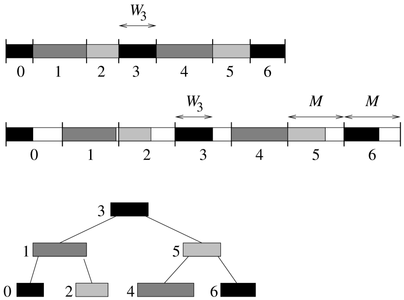
Figure 4.2: Weighted (top), uniform (middle), and hierarchical (bottom) selection. For the weighted selection the cumulative length of the bars has to be added. In the uniform selection a bar is randomly selected and then accepted with probability $W_{n}/M$. In the hierarchical selection each node has the sum of the lengths of all bars in the subtree, and we need only to go down the tree to make the selection.

It is possible to do the weighted selection of the reactions also in $O(\log S)$ time by using a binary tree.[59] Each node of the tree has a reaction and the cumulative rate constant of all reactions of the node and both branches below the node. After $rk_{\alpha}$ has been determined we look for the node with $C_{\rm left}<rk_{\alpha}\leq C_{\rm left}+W_{\rm node}$ where $W_{\rm node}$ is the rate constant of the reaction of the node and $C_{\rm left}$ is the cumulative rate constant of the top node of the left branch. If there is no left branch then we define $C_{\rm left}=0$. To find the node we do we do the following.

1. Start

   Set $X=rk_{\alpha}$.

   Take the top node of the tree.

2. Reaction found?

   if $C_{\rm left}<X\leq C_{\rm left}+W_{\rm node}$

   then stop; take the reaction of the node.

   else go to the next step

3. Continue in the left branch?

   if $X\leq C_{\rm left}$

   then take the top node of the left branch and continue at step 2

   else go to the next step

4. Continue in the right branch.

   Set $X\to X-(C_{\rm left}+W_{\rm node})$.

   Take the top node of the right branch and continue at step 2.

The number of nodes we have to inspect is equal to the depth of the tree. If the tree is well-balanced this is $O(\log S)$. We can use this method also for a weighted selection of the reaction type, if the number of reaction types is large. In fact this occurs in DMC simulations of reactions in solutions and the method we describe here is one method that is used for these simulations.[50]

4.1.5 Handling disabled reactions.

The problem of removing disabled reactions has a surprisingly simple solution, although it is a bit more difficult to see that it is also a correct solution. Instead of removing the disabled reactions, we simply leave them in the list of all reactions, but when a reaction has to occur we check if it is disabled. If it is we remove it. If it is an enabled reaction, we treat it as usual. That this is correct can be proven as follows. Suppose that $k_{\rm en}$ is the sum of the rate constants of all enabled reactions, and we have one disabled reaction with rate constant $k_{\rm dis}$. Also suppose without loss of generality that the system is at time $t=0$. The probability distribution for the first reaction to occur is $k_{\rm en}\exp(-k_{\rm en}t)$ (see equation (4.8)). If we work with the list that includes the disabled reaction than the probability distribution for the first reaction occurring at time $t$ being also an enabled reaction is $k_{\rm en}\exp(-(k_{\rm en}+k_{\rm dis})t)$, which is the probability that no reaction occurs until time $t$ and then an enabled reaction occurs. This is the first contribution to the probability distribution for the enabled reaction if the disabled reaction is not removed. The probability distribution that the first reaction is not but the second reaction is enabled and occurs at time $t$ is given by

$$k_{\rm en}\int_{0}^{t}\!\!dt^{\prime}\,e^{-k_{\rm en}(t-t^{\prime})}k_{\rm dis}e^{-(k_{\rm en}+k_{\rm dis})t^{\prime}}$$

$$=k_{\rm en}e^{-k_{\rm en}t}k_{\rm dis}\int_{0}^{t}\!\!dt^{\prime}\,e^{-k_{\rm dis}t^{\prime}}$$

$$=k_{\rm en}e^{-k_{\rm en}t}\left[1-e^{-k_{\rm dis}t}\right].$$ (4.14)

Adding this to $k_{\rm en}\exp(-(k_{\rm en}+k_{\rm dis})t)$ gives us $k_{\rm en}\exp(-k_{\rm en}t)$, which is what we should have.

This shows that adding a single disabled reaction does not change the probability distribution for the time that the first enabled reaction occurs. In the same way we can show that adding a second disabled reaction gives the same probability distribution as having a single disabled reaction, and that adding a third disabled reaction is the same as having two disabled reactions, etc. So by induction we see that disabled reactions do not change the probability distribution for the occurrence of the enabled reactions. Also step 3 of VSSMi is no problem. The enabled reactions are chosen with a probability proportional to their rate constant whether or not disabled reactions are present in he list.

The VSSM algorithm now gets the following form.

Variable Step Size Method with an approximate list of reactions (VSSMa)

1. Initialize

   Generate an initial configuration $\alpha$.

   Make lists $L_{\rm rx}^{(i)}$ containing all reactions of type $i$.

   Calculate $k^{(i)}\equiv N^{(i)}W^{(i)}$, with $N^{(i)}$ the number of reactions of type $i$ and $W^{(i)}$ the rate constant of these reactions.

   Set the time $t$ to some initial value.

   Choose conditions when to stop the simulation.

2. Reaction time

   Generate a time interval $\Delta t$ when no reaction takes place

   $$\Delta t=-{1\over\sum_{i}k^{(i)}}\ln r,$$ (4.15)

   where $r$ is a random deviate on the unit interval.

   Change time to $t\to t+\Delta t$.

3. Reaction

   Pick a type of reaction $j$ with probability $k^{(j)}/\sum_{i}k^{(i)}$, and then pick the reaction $\beta\to\alpha^{\prime}$ from $L_{\rm rx}^{(j)}$ at random. If the reaction is enabled go to step 4. If it is disabled go to step 6. (Note that during the simulation $k^{(j)}$ may have obtained contributions from disabled reactions starting from configurations different from $\alpha$.)

4. Enabled reaction

   Change the configuration to $\alpha^{\prime}$.

5. Enabled update

   Remove the reaction $\beta\to\alpha^{\prime}$ from $L_{\rm rx}^{(j)}$. Change $k^{(j)}\to k^{(j)}-W^{(j)}$. (Note that because the reaction is enabled $\beta=\alpha$.)

   Add new enabled reactions to the lists $L_{\rm rx}^{(i)}$.

   Use these reactions to calculate the new values for $k^{(i)}$ from the old ones.

   Skip to step 8.

6. Disabled reaction

   Do not change the configuration; $\alpha^{\prime}$ is the same configuration as $\alpha$.

7. Disabled update

   Remove the disabled reaction from $L_{\rm rx}^{(j)}$.

   Change $k^{(j)}\to k^{(j)}-W^{(j)}$.

8. Continuation

   If the stop conditions are fulfilled then stop. If not repeat at step 2.

The computer time per reaction of algorithm VSSMa scales as $O(1)$. This is achieved by working with an approximate list of all reactions; a list that can contain disabled reactions. We will see that the same trick can be used with other algorithms as well. Note that picking the reaction type at step 3 can be done hierarchically as explained at the end of section 4.1.4.

4.1.6 Reducing memory requirements.

There are other ways we might want to change the VSSM algorithm, but then because of memory considerations. The description of the algorithms uses a list of all reactions. This list is quite large and scales with system size. We can do away with this list at the cost of increasing computer time, although the algorithm will still scale as $O(1)$.

Instead of keeping track of all individual reactions we only keep track of how many reactions there are of each different type; i.e., no lists $L_{\rm rx}^{(i)}$ but only the numbers $N^{(i)}$. Because there are no lists we have to count how many reactions become disabled after a reaction has occurred. This is similar to adding enabled reactions and can be done in constant time. (Note that this is only because we are using no lists. Removing disabled reactions from lists is what costs time.) This means that the number $N^{(i)}$ will be exact. The only problem is, after the type of reaction is determined, how to determine which particular reaction will take place. This can be done by randomly searching on the surface. The number of places one has to look does not depend on the system size, but on the probability that the reaction can occur on a randomly selected site. This random search for the location of the reaction is another form of uniform selection. Another application of such a uniform selection will be given in section 4.1.9. If the type of reaction can take place on many places, then a particular reaction should rapidly be found.

To make the formulation of the new algorithm not too difficult we use a more restrictive definition of a reaction type, in the sense that two reactions are of the same type if one can be obtained from to other by a translation. Previously we also talked about the same reaction type if the orientation was different. We don’t do this here, because we want to have an unambiguous meaning if we say that a reaction occurs at a particular site (see step 4 of VSSMs) even if more sites are involved. For example, if we have a reaction type of an A reacting with a B where the B is at a site to the right of the A, then by the site of this reaction we mean the site where the A is. The new algorithm then becomes as follows.

Variable Step Size Method with random search for the location of reactions (VSSMs).

1. Initialize

   Generate an initial configuration.

   Count how many reactions $N^{(i)}$ of type $i$ there are.

   Calculate $k^{(i)}\equiv N^{(i)}W^{(i)}$, with $W^{(i)}$ the rate constant of the reactions of type $i$.

   Set the time $t$ to some initial value.

   Choose conditions when to stop the simulation.

2. Reaction time

   Generate a time interval $\Delta t$ when no reaction takes place

   $$\Delta t=-{1\over\sum_{i}k^{(i)}}\ln r,$$ (4.16)

   where $r$ is a random deviate on the unit interval.

   Change time to $t\to t+\Delta t$.

3. Reaction type

   Pick a type of reaction $j$ with probability $k^{(j)}/\sum_{i}k^{(i)}$.

4. Reaction location

   Pick randomly a site for the reaction, until a site is found where the reaction can actually occur.

5. Update

   Change the configuration.

   Determine the new enabled reactions, and change the $N^{(i)}$’s accordingly.

   Determine the disabled reactions, and change the $N^{(i)}$’s accordingly.

6. Continuation

   If the stop conditions are fulfilled then stop. If not repeat at step 2.

4.1.7 Oversampling and the Random Selection Method.

The determination of a reaction and its time can be split in three parts; the time of the reaction, the type of the reaction, and the site of the reaction. The last two parts were combined in the previous versions of VSSM. The determination of the reaction type has to be done before the determination of the location of the reactions in VSSMs (otherwise one doesn’t know when to stop searching in step 4), but the time of the reaction can be determined independently from which reactions occurs where. It is also possible to determine all three parts independently. This has the advantage that even less bookkeeping is necessary; adding and removing reactions to update lists or numbers of types of reaction is not necessary. The drawback is however the same as in VSSMs, only worse; as in step 4 of VSSMs reactions will be attempted at certain locations where the reactions cannot take place. If this does not occur to often, then this drawback may be small.

The trick to do away with the bookkeeping is to use a technique called oversampling. Suppose we have just one type of reaction and that we have $N$ of them. (A reaction type is defined here in the same way as for VSSMs.) The time to the next occurrence of a reaction is then given the probability distribution $NW\exp(-NWt)$ where $W$ is the rate constant of the reaction. If we assume, however, that we have $M$ of these reactions with $M>N$ then we can also generate the time of the next reaction from the distribution $MW\exp(-MWt)$, but then accept the reaction with probability $N/M$. To prove this we need to add the contributions that the reaction has to be generated one, two, three etc. times before one is found that is accepted.

$${N\over M}MW\exp(MWt)$$

$$+\int_{0}^{t}\!\!dt^{\prime}\,{N\over M}MWe^{-MW(t-t^{\prime})}\left[1-{N\over M}\right]MWe^{-MWt^{\prime}}$$

$$+\int_{0}^{t}\!\!dt^{\prime}\int_{0}^{t^{\prime}}\!\!dt^{\prime\prime}\,{N\over M}MWe^{-MW(t-t^{\prime})}$$

$$\qquad\times\left[1-{N\over M}\right]MWe^{-MW(t^{\prime}-t^{\prime\prime})}\left[1-{N\over M}\right]MWe^{-MWt^{\prime\prime}}+\ldots$$

$$=NWe^{-MWt}\left[1+\left[1-{N\over M}\right]MWt+{1\over 2}\left[1-{N\over M}\right]^{2}M^{2}W^{2}t^{2}+\ldots\right]$$

$$=NWe^{-MWt}e^{[1-N/M]MWt}=NWe^{-NWt}.$$ (4.17)

The following algorithm is only useful if we do not need to determine $N$ explicitly. This can be accomplished if we assume that all reaction types can take place everywhere on the surface. In terms of lists this means that each list $L_{\rm rx}^{(i)}$ has the same $S$ reactions during an entire simulation. Because the lists do not change and they have a simple definition, we do not need to determine them explicitly. Also the times of the reactions are always taken from the same probability distribution, and the probabilities to choose a reaction type do not change. The algorithm looks as follows.

Random Selection Method (RSM).

1. Initialize

   Generate an initial configuration.

   Set the time $t$ to some initial value.

   Define $k\equiv SW_{\rm max}$ where $W_{\rm max}$ is the maximum of the rate constants $W^{(i)}$’s of type $i$.

   Choose conditions when to stop the simulation.

2. Reaction time

   Generate a time interval $\Delta t$ when no reaction takes place

   $$\Delta t=-{1\over k}\ln r,$$ (4.18)

   where $r$ is a random deviate on the unit interval.

3. Reaction type

   Pick a type of reaction randomly.

4. Reaction location

   Pick a site randomly.

5. Update

   Change time to $t\to t+\Delta t$.

   If the reaction is possible at the site from step 4, then accept the reaction with probability $W^{(i)}/W_{\rm max}$ where $i$ is the type of reaction from step 3

   If the reaction is possible and accepted, change the configuration.

6. Continuation

   If the stop conditions are fulfilled then stop. If not repeat at step 2.

This algorithm is called the Random Selection Method (RSM). Note that the reaction time, the type of the reaction, and the location of the reaction can be done in any order. Only time and the configuration of the system needs to be updated. The method is therefore very efficient, provided that in step 5 reaction are accepted often.

4.1.8 The First Reaction Method.

Instead of splitting the time, the type, and the location of a reaction, it is also possible to combine them. This is done in the First Reaction Method.

The First Reaction Method (FRM)

1. Initialize

   Generate an initial configuration $\alpha$.

   Set the time $t$ to some initial value.

   Make a list $L_{\rm rx}$ containing all reactions.

   Generate for each reaction $\alpha\to\beta$ in $L_{\rm rx}$ a time of occurrence

   $$t_{\beta\alpha}=t-{1\over W_{\beta\alpha}}\ln r$$ (4.19)

   with $W_{\beta\alpha}$ the rate constant for the reaction and $r$ a random deviate on the unit interval.

   Choose conditions when to stop the simulation.

2. Reaction

   Take the reaction $\alpha\to\alpha^{\prime}$ with $t_{\alpha^{\prime}\alpha}\leq t_{\beta\alpha}$ for all $\beta$.

   If the reaction is enabled go to step 3. If not go to step 4.

3. Enabled update

   Change the configuration to $\alpha^{\prime}$.

   Change time to $t\to t_{\alpha^{\prime}\alpha}$

   Remove the reaction $\alpha\to\alpha^{\prime}$ from $L_{\rm rx}$.

   Add new enabled reactions to $L_{\rm rx}$ and generate for each reaction $\alpha^{\prime}\to\beta$ a time of occurrence

   $$t_{\beta\alpha^{\prime}}=t-{1\over W_{\beta\alpha^{\prime}}}\ln r.$$ (4.20)

   Skip to step 5.

4. Disabled update

   Do not change the configuration: $\alpha^{\prime}$ is the same configuration as $\alpha$.

   Remove the disabled reaction from $L_{\rm rx}$.

5. Continuation

   If the stop conditions are fulfilled then stop. If not set $\alpha$ to $\alpha^{\prime}$ and repeat at step 2.

This algorithm is called Discrete Event simulation in computer science.[60] In FRM the determination of the type and the site of a reaction is replaced by comparing times of occurrences for individual reactions. That this is correct can be seen as follows. Suppose we have two reactions with rate constants $W_{1}$ and $W_{2}$. The probability that no reaction occurs in the interval $[0,t]$ is then $\exp[-(W_{1}+W_{2})t]$, whereas the probability that neither reaction 1 nor reaction 2 occurs in that interval equals $\exp(-W_{1}t)\exp(-W_{2}t)$, which is obviously the same as the previous expression. This proves that FRM generates correct reaction times. It’s a bit more work to show that the reactions are chosen with the correct probability. The probability distribution for the reactions times of the reactions are $W_{i}\exp(-W_{i}t)$ with $i=1,2$. The probability that reaction 1 occurs before reaction 2 in the FRM algorithm is given by

$$\int_{0}^{\infty}\!\!dt\,W_{1}e^{-W_{1}t}\int_{t}^{\infty}\!\!dt^{\prime}W_{2}e^{-W_{1}t^{\prime}}$$ (4.21)

$$\quad=W_{1}\int_{0}^{\infty}\!\!dt\,e^{-W_{1}t}e^{-W_{2}t}={W_{1}\over W_{1}+W_{2}}.$$

For reaction 2 we find $W_{2}/(W_{1}+W_{2})$, which shows that FRM also picks the reactions with the correct probability. So we see that one can either generate one time for all reactions and then choose one reaction, or generate times for all reactions and then take the first that will occur. We will use this later on in another way.

The disadvantage of FRM is the determination of the reaction with the smallest time of occurrence. Scanning a list of all reaction for each new reaction scales as $O(S)$. More efficient is to make the list of all reactions an ordered one, and keep it ordered during a simulation. Getting the next reaction scales then as $O(1)$, but inserting new reactions in $L_{\rm rx}$ scales as $O(\log S)$.[59] This is not as good as constant time, but it is not particularly bad either. Still VSSM is often more efficient than FRM, but VSSM cannot always be used as we will show later, whereas FRM can always be used.

Note that disabled reactions are not removed from the list of all reactions. Note also that we only have to generate reaction times for the new enabled reactions. Times for reactions already in $L_{\rm rx}$ need not be generated again. Suppose that at time $t=t_{1}$ a time has been generated for a reaction with rate constant $W$. The probability distribution for that time is $W\exp[-W(t-t_{1})]$. Now assume that at time $t=t_{2}>t_{1}$ the reaction has not occurred. We might generate a new time using the new probability distribution $W\exp[-W(t-t_{2})]$. However, the ratio of the values of these probability distributions for times $t>t_{2}$ is $W\exp[-W(t-t_{2})]/W\exp[-W(t-t_{1})]=\exp[W(t_{2}-t_{1})]$ is a constant. Hence relative probabilities for the times $t>t_{2}$ that the reaction can occur are the same for both probability distributions, and no new time need to be generated.

4.1.9 Practical considerations

There are different aspects to consider by people who just want to use the algorithms above to simulate a particular reactions system, and by people who want to implement them. For the implementation the efficiency of the methods described above depends very much on details of the algorithm that we have not discussed. However, some general guidelines can and will be given here. The interested reader is referred to references [61] and [62] for a more extensive analysis.

An important point is that memory and computation time depend mainly on the data structures that are used. Except for the time steps there is relatively little to really calculate. This involves the generation of a random number. Random numbers are also needed to pick reactions or reaction types and sites. More critical are the data structures that contain the reactions and/or reaction types. These lists are priority queues,[59] and in particular for FRM these may become quite large. A problem are the disabled reactions. Removing them depends linearly on the size of the lists and is generally inefficient, and should not be done after each reaction. It is better to remove them only when they should occur, and it is found that they have become disabled. Alternatively, one can do garbage collection when the size of the list becomes too large.[63] The determination of the next reaction that should occur depends only logarithmically on the size of the list in FRM. In VSSM and RSM this can even be done in constant time.

There are a few other aspects that are important and that we haven’t mentioned yet. A central step in all algorithms is the determination of what are the new reactions that have become possible just after a reaction has occurred. There are dependencies between the reactions that may be used to speed up the simulation. A small example may make this clearer. Suppose we have just adsorption of A or B onto vacant sites, and formation of AB from an A next to a B leaving two vacant sites. The formation of an AB will allow new A and B adsorptions, but no new AB formation. So it is not necessary to check if any AB formations have become enabled.

Testing if a reaction is disabled is not trivial. It won’t do to see if the occupation of the relevant sites allows the reaction to occur. It may be that the occupation of the sites has changed a few times but then converted back to a situation so that the reaction can occur again. What has happened then is that when the reaction became enabled for the second time it was added to the list of reactions for the second time too. If the first instance of the reaction on the list is not recognized as disabled, then the reaction will take place at the first time of occurrence. This means that effectively the reaction has a double rate constant. This is similar to oversampling (section 4.1.7) and accepting each reaction with probability 1. (This problem does not occur, of course, in VSSMs and in RSM.)

Recognizing that a reaction is disabled can be done by keeping track of when a reaction became enabled and when the occupation of a site last changed. If a site involved in the reaction changed after the reaction became enabled, then the reaction should be regarded as being disabled. Using the times of these changes may however lead to problems because of rounding errors in the representation of real (floating point) numbers. Instead one can use integers that count reactions when they become enabled. Each reaction is assigned then its count number, and each site is assigned the number of the reaction that last changed it. It a site involved in a reaction has a number larger than the number of the reaction, then the reaction is disabled.

From the point of view of using the algorithms to simulate a system an important aspect seems to be the scaling with system size. The important difference between FRM on the one, and VSSM (i.e., VSSMa and VSSMs) and RSM on the other hand is the dependence on the system size. Computer time per reaction in VSSM and RSM does not depend on the size of the system. This is because in these methods picking a reaction is done using uniform selection, which does not depend on the size of the list of reactions. In RSM there is not even such a list. In FRM the computer time per reaction depends logarithmically on the system size. Here we have to determine which of all reactions will occur first. So for large systems VSSM and RSM are generally to be preferred. The data structure of FRM is so time consuming that FRM should only be used if really necessary.

There are however a number of cases that occur quite frequently in which VSSM and RSM are not efficient. This is when there are many reaction types and when the rate constants depend on time. Time-dependent rate constants will be discussed in section 4.1.10. Many reaction types arise, for example, when there are lateral interactions. In this case VSSM becomes inefficient because it will take a lot of time to determine the reaction type. If with the lateral interactions many adsorbates affect the rate constant of a reaction, then the number of reaction types easily becomes larger than the number of sites (see section 5.7). RSM can be used for lateral interactions, provided that the effect of them is small. With RSM one need only include in the reaction description those sites for which the occupancy changes. If one also includes the sites with the adsorbates affecting the rate constants then the probability that one picks a reaction type that can occur at the randomly chosen site is too low. The adsorbates affecting the rate constants should, of course, be included when one calculates the rate constant for the determination of the acceptance of a reaction. If the effect of lateral interactions is large then this acceptance will often be low, and RSM will not be very efficient. This is very often the case. In general, one should realize that simulations of systems with lateral interactions are always costly.

If VSSM and RSM can be used, then the choice between them depends on how many sites in the system the reactions can occur. RSM is efficient for reactions that occur on many sites. The probability that a reaction is possible on the randomly chosen location is then high. If this is not the case then VSSM should be used.

The choice between FRM, VSSM, and RSM need not be made for all reactions in a system together, but can be made on a per reaction type basis, because it is easy to combine the different methods. Suppose that reaction type 1 is best treated by VSSM, but reaction type 2 best by RSM. We then determine the first reaction of type 1 using VSSM, and the first of type 2 by RSM. The first reaction to actually occur is then simply the first reaction of these two. The proof that this is correct is identical to the proof of the correctness of FRM. Combining algorithms in this way can be particularly advantageous for models with many reaction types.

To summarize, VSSM is generally the best method to use unless the number of reaction types is very large. In that case use FRM. If you have a reaction that occurs almost everywhere, RSM should be considered. Simply doing the simulation with different methods and comparing is of course best. One should also look for alternative ways to model the system (see chapter 5).

4.1.10 Time-dependent transition probabilities.

If the transition probabilities $W_{\alpha\beta}$ are themselves time dependent, then the integral formulation above needs to be adapted. This situation arises, for example, when dealing with Temperature-Programmed Desorption or Reactions (TPD/TPR),[43, 64, 65] and when dealing with voltammetry.[66] The definition of the matrices ${\bf W}$ and ${\bf R}$ remains the same, but instead of a matrix ${\bf Q}(t)$ we get

$${\bf Q}(t^{\prime},t)\equiv\exp\left[-\int_{t}^{t^{\prime}}\!\!dt^{\prime\prime}\,{\bf R}(t^{\prime\prime})\right].$$ (4.22)

With this new ${\bf Q}$ matrix the integral formulation of the Master Equation becomes

$${\bf P}(t)=\bigg{[}{\bf Q}(t,0) + \int_{0}^{t}\!\!dt^{\prime}{\bf Q}(t,t^{\prime}){\bf W}(t^{\prime}){\bf Q}(t^{\prime},0)$$

$$+ \int_{0}^{t}\!\!dt^{\prime}\int_{0}^{t^{\prime}}\!\!dt^{\prime\prime}{\bf Q}(t,t^{\prime}){\bf W}(t^{\prime}){\bf Q}(t^{\prime},t^{\prime\prime}){\bf W}(t^{\prime\prime}){\bf Q}(t^{\prime\prime},0)+\ldots\bigg{]}{\bf P}(0).$$

The interpretation of this equation is the same as that of equation (4.1.1). This means that it is also possible to use VSSM to solve the Master Equation. The relevant equation to determine the times of the reactions becomes

$${\bf Q}(t_{n},t_{n-1})=r,$$ (4.24)

where $t_{n-1}$ is the time of the last reaction that has occurred, and the equation should be solved for $t_{n}$, which is the time of the next reaction. If just after $t_{n-1}$ the system is in configuration $\alpha_{n-1}$, then the next reaction leading to configuration $\alpha_{n}$ should be picked out off all possible reaction with probability proportional to $W_{\alpha_{n}\alpha_{n-1}}(t_{n})$.

The drawback of VSSM for time-dependent transition probabilities is that the equation for the times of the reactions is often very difficult to be solved efficiently. Equation (4.24) can in general not be solved analytically, but a numerical solution with a $Q$ of the form shown in figure 4.3 is also not easy. The problem is that ${\bf R}$ in equation (4.22) can contain many terms or terms that have a very different time dependence due to reactions with different activation energy. A possible solution is to use VSSM for each reaction type separately; i.e., we solve equation (4.24) for each reaction type separately. The next reaction is then of the type with the smallest value for $t_{n}$, and the first reaction is chosen from those of that type as in VSSM.[62] This works provided the number of reaction types is small.

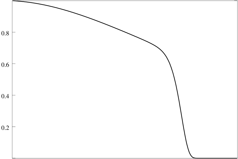
Figure 4.3: Sketch of the probability that no reaction has taken place as a function of time typically for a Temperature-Programmed Desorption spectrum. The slow initial decrease is due to a reaction with a small activation energy and preexponential factor. The large decrease at the end is due to a reaction with a high activation energy and preexponential factor.

Instead of computing a time for the next reaction using the sum of the transition probabilities of all possible reactions, we can also compute a time for each reaction. So if we’re currently at time $t$ and in configuration $\alpha$, then we compute for each reaction $\alpha\to\beta$ a time $t_{\beta\alpha}$ using

$$\exp\left[-\int_{t}^{t_{\beta\alpha}}\!\!dt^{\prime}\,W_{\beta\alpha}(t^{\prime})\right]=r,$$ (4.25)

where $r$ is again a uniform deviate on the unit interval. The first reaction to occur is then the one with the smallest $t_{\beta\alpha}$. It can be shown that this time has the same probability distribution as that of VSSM just as for time-independent rate constants. This method is FRM for time-dependent reaction rate constants.[43]

The equations defining the times for the reactions, equation (4.25), are often much easier to solve than equation (4.24). It may seem that this is offset by the fact that the number of equations (4.25) that have to be solved is very large, but that is not really the case. Once one has computed the time of a certain reaction, it is never necessary to compute the time of that reaction again, but one can use the time that one has computed at the moment during the simulation when the reaction has become possible just as for the case of time-independent rate constants.

Equation (4.25) can have an interesting property, which is that it may have no solution. The expression

$$P_{\rm not}(t)\equiv\exp\left[-\int_{t_{\rm now}}^{t}\!\!dt^{\prime}\,W_{\beta\alpha}(t^{\prime})\right]$$ (4.26)

is the probability that the reaction $\alpha\to\beta$ has not occurred at time $t$ if the current time is $t_{\rm now}$. As $W_{\beta\alpha}$ is a non-negative function of time, this probability decreases with time. It is bound from below by zero, but it need not go to zero for $t\to\infty$. If it does not, then there is no solution when $r$ is smaller than $\lim_{t\to\infty}P_{\rm not}(t)$. This means that there is a finite probability that the reaction will never occur. This is the case with some reaction in cyclic voltammetric experiments.[66] There is always a solution if the integral goes to infinity. This is the case when $W_{\beta\alpha}$ goes slower to zero than $1/t$, or does not go to zero at all.

4.2 A comparison with other methods.

There are a few other approaches that we want to mention here. The fixed time step method discretized time. The algorithmic methods are older methods that are still being used. Kinetic Monte Carlo is very similar to VSSM and is quite popular. Cellular Automata are mentioned also but only briefly, as they are really outside the scope of this introduction to MC methods.

4.2.1 The fixed time step method

If we discretize time then the Master Equation can be written as

$$P_{\alpha}(t+\Delta t)=P_{\alpha}(t)+\sum_{\beta}\left[W_{\alpha\beta}\Delta t\,P_{\beta}(t)-W_{\beta\alpha}\Delta t\,P_{\alpha}(t)\right].$$ (4.27)

This means that if at time $t$ we are in configuration $\alpha$, then at time $t+\Delta t$ we are still in configuration $\alpha$ with probability $1-\sum_{\beta}W_{\beta\alpha}\Delta t$ and in configuration $\beta$ different from $\alpha$ with probability $W_{\beta\alpha}\Delta t$. This leads to the following algorithm. For each reaction $\alpha\to\beta$ we generate a random number between 0 and 1. If $r\leq W_{\beta\alpha}\Delta t$ then we change the configuration to $\beta$ and time to $t+\Delta t$. If $r>W_{\beta\alpha}\Delta t$ then we only change time to $t+\Delta t$.

The algorithm above can be very efficient if it works. For example, if the rate constants are time dependent, then the fixed time step method assumes that it is constant during the interval $[t,t+\Delta t]$. This avoids the evaluation of integrals like (4.25). However, it is obviously an approximation, which might necessitate small time steps. The time step also has to be small because the probabilities $W_{\beta\alpha}\Delta t$ and $1-\sum_{\beta}W_{\beta\alpha}\Delta t$ must be between 0 and 1. Determining the maximum $\Delta t$ that gives correct results might be cumbersome.

A more subtle problem is that one should avoid the possibility that two reactions cannot both occur but for both holds $r\leq W_{\beta\alpha}\Delta t$. For example, an adsorbate can desorb or react with a neighbor. The adsorbate cannot do both, but if for both reactions we find $r\leq W_{\beta\alpha}\Delta t$, then we have a problem. In practice this means that $\Delta t$ should be chosen so small that at most one reaction occurs during each time step.

4.2.2 Algorithmic approach

Almost all older Dynamic Monte Carlo methods are based on an algorithm that defines in what way the configuration changes. (A nice review with many references to work with these methods is reference [67].) The generic form of that algorithm consists of two steps. The first step is to pick a site. The second step is to try all reactions at that site. (This may involve picking additional neighboring sites.) If a reaction is possible at that site, then it is executed with some probability that is characteristic for that reaction. These two steps are repeated many times. The sites are generally picked at random. In a variant of this algorithm just one reaction is tried until on average all sites have been visited once, and then the next reaction is tried, etc. This variant is particular popular in situations with fast diffusion; the “real” reactions are tried first on average once on all sites, and then diffusion is used to equilibrate the system before the next cycle of “real” reactions.

These algorithmic Dynamic Monte Carlo methods have provided very valuable insight in the way the configuration of the adsorbates on a catalyst evolves, but they have some drawbacks. First of all there is no real time. Instead time is specified in so-called Monte Carlo steps (MCS). One MCS is usually defined as the cycle in which every site has on average been visited once for each reaction. The second drawback is how to choose the probabilities for reactions to occur. It is clear that faster reactions should have a higher probability, but it is not clear how to quantify this. This drawback is related to the first. Without a link between these probabilities and microscopic reaction rate constants it is not possible a priori to tell how many real seconds one MCS corresponds to. The idea is that Monte Carlo time in MCS and real time are proportional. We have used the similarity with RSM and shown that this is indeed the case provided temporal fluctuations are disregarded and one has a steady state. In the case of, for example, oscillations the two time scales are not proportional.[61] In practice people have used the algorithmic approach to look for qualitative changes in the behavior of the system when the reaction probabilities are varied, or they have fitted the probabilities to reproduce experimental results.

The third drawback is that it is difficult with this algorithmic definition to compare with other kinetic theories. Of course, it is possible to compare results, but an analysis of discrepancies in the results is not possible as a common ground (e.g., the Master Equation in our approach) is missing. The generic form of the algorithm described above resembles the algorithm of RSM. Indeed one may look upon RSM as a method in which the drawbacks of the algorithmic approach have been removed.

4.2.3 Kinetic Monte Carlo

The problem of real time in the algorithmic formulation of Dynamic Monte Carlo has also been solved by Fichthorn and Weinberg.[54] Their method is called Kinetic Monte Carlo (KMC) and has become quite popular. They replaced the reaction probabilities by rate constants, and assumed that the probability distribution $P_{\rm rx}(t)$ of the time that a reaction occurs is a Poisson process; i.e., it is given by

$$P_{\rm rx}(t)=k\exp[-k(t-t_{\rm now})],$$ (4.28)

where $t_{\rm now}$ is the current time, and $k$ is the rate constant. Using the properties of this distribution they derived a method that is really identical to our VSSM, expect in two aspects. One aspect is that the Master Equation is absent, which makes it again difficult to make a comparison with other kinetic theories. Instead the method was derived by asking under which conditions an equilibrium MC simulation can be interpreted as a temporal evolution of a system. The other aspect is that time is incremented deterministically using the expectation value of the probability distribution of the first reaction to occur; i.e.,

$$\Delta t={1\over\sum_{i}N_{i}k_{i}},$$ (4.29)

where $k_{i}$ is the rate constant of reaction type $i$ (this is the same as our transition probabilities $W$ in equation (2.4)), and $N_{i}$ is the number of reaction of type $i$. This avoids having to solve equation (4.10), and has been used subsequently by many others. However, as solving that equation only involves generating a random number and a logarithm, which is a negligible contribution to the computer time, this is not really an advantage. Equation (4.29) does neglect temporal fluctuations, which may be incorrect for systems of low dimensionality.[68]

Although the derivation of Fichthorn and Weinberg only holds for Poisson processes, their method has also been used to simulate TPD spectra.[56] In that work it was assumed that, when $\Delta t$ computed with equation (4.29) is small, the rate constants are well approximated over the interval $\Delta t$ by their values at the start of that interval. This seems plausible, but, as the rate constants increase with time in TPD, equation (4.29) systematically overestimates $\Delta t$, and the peaks in the simulated spectra are shifted to higher temperatures. In general, if the rate constants are time dependent then it may not even be possible to define the expectation value. We have already mentioned the case of cyclic voltammetry where there is a finite probability that a reaction will not occur at all. The expectation value is then certainly not defined. Even if a reaction will occur sooner or later the distribution $P_{\rm rx}(t)$ has to go faster to zero for $t\to\infty$ than $1/t^{2}$ for the expectation value to be defined. Solving equations (4.10) or (4.25) does not lead to such problems.

4.2.4 Cellular Automata

There is an extensive literature on Cellular Automata. A discussion of this is outside the scope of this chapter, and we will restrict ourselves to some general remarks. We will also restrict ourselves to Cellular Automata in which each cell corresponds to one site. The interested reader is referred to references[69, 70, 71, 72, 73, 74] for an overview of the application of Cellular Automata to surface reactions.

The main characteristic of Cellular Automata is that each cell, which corresponds to a grid point in our model of the surface, is updated simultaneously. This allows for an efficient implementation on massive parallel computers. It also facilitates the simulation of pattern formation, which is much harder to simulate with some asynchronous updating scheme as in Dynamic Monte Carlo.[75] The question is how realistic a simultaneous update is, as a reaction seems to be a stochastic process. One has tried to incorporate this randomness by using so-called probabilistic Cellular Automata, in which updates are done with some probability. These Cellular Automata differ little from Dynamic Monte Carlo. In fact, probabilistic Cellular Automata can be made that are equivalent to the RSM algorithm.[62]

4.3 The CARLOS program

CARLOS is a general purpose program for surface reactions.[76] It was developed by Johan Lukkien at the Eindhoven University of Technology in the Netherlands. General purpose means that it does not have any reaction hard-coded, but one can specify almost any type of reaction on input. For time-independent rate constants one can choose between VSSM, RSM, and FRM. With time-independent rate constants the different methods can be combined in one simulation. For time-dependent rate constants only FRM can be used. Each rate constant $W$ can be specified as a constant or as

$$W=\nu e^{-E{\rm act}/k_{\rm B}T},$$ (4.30)

and the preexponential factor $\nu$, the activation energy $E_{\rm act}$, and the temperature $T$ are to be given on input. These quantities can be linear functions of time. In this way one can simulate TPD/TPR experiments ($T$ a function of time) and linear sweep voltammetry experiments ($E_{\rm act}$ a function of time). One can also change any quantity in discrete steps. This allows the use of VSSM and RSM for rate constants with arbitrary time dependence, although strictly speaking only approximately.

CARLOS uses pattern recognition for finding which reactions are possible. Each reaction has to be specified as a list of sites involved in the reaction, the occupation of the sites before, and the occupations of them after the reaction has taken place. For example, in

$$(0,0),(1,0):\hbox{ A B}\to\hbox{$*$ $*$}$$ (4.31)

an integer pair $(n_{1},n_{2})$ indicates a unit cell, A and B are reactions, and $*$ the product. This can be interpreted as an molecule A reacting with a molecule B at a neighboring site to form AB which immediately desorbs leaving two vacant sites. This interpretation, however, is based on the meaning of the labels A, B, and $*$. CARLOS does not know this meaning so the interpretation is ultimately up to the user. CARLOS only searches for a pattern on the left of the arrow and changes it to the pattern on the right. The labels can also be used to indicate different substrate atoms, types of sites (sites with different coordination numbers, defect sites, step sites, etc.), or surface reconstruction.

The indices specifying the unit cells are relative. The specification above stands not just for a reaction at $(0,0)$ and $(1,0)$, but at $(n_{1},n_{2})$ and $(n_{1}+1,n_{2})$ for any integers $n_{1}$ and $n_{2}$. Having more than one site per unit cell is also possible. For example in

$$(0,0/0),(0,0/1):\hbox{ A B}\to\hbox{$*$ $*$}$$ (4.32)

the reaction takes place on two sites in the same unit cell. The integers after the slash indicate which sites are involved. CARLOS does not make any assumptions on distances or angles. So

$$(0,0),(1,0):\hbox{ A B}\to\hbox{$*$ $*$}$$ (4.33)

may refer to a square, a hexagonal, or any other type of lattice. However, to simplify the specification of many symmetry related reactions, one can specify this symmetry, and then CARLOS does assume certain conventions in the specification of the sites. For example, the lines Active sites: top on hex $\vdots$ $\vdots$ Symmetry: hex 120 $\ldots$ $(0,0),(1,0):\hbox{ A B}\to\hbox{$*$ $*$}$ on input make CARLOS assume that the lattice is hexagonal, and that the primitive translation vectors have the same length and make an angle of $60^{\circ}$. Apart from the reaction explicitly stated above, CARLOS will also generate

$$(0,0),(-1,1):\hbox{ A B}\to\hbox{$*$ $*$}$$ (4.34)

and

$$(0,0),(0,-1):\hbox{ A B}\to\hbox{$*$ $*$},$$ (4.35)

which are obtained by rotations of $120^{\circ}$.

As output CARLOS can generate a list of coverages and rates as a function of time. This list contains all possible information on the kinetics. The configuration of a system as a function of time can be shown on screen and/or sent to a file either in graphic format or in a format that CARLOS can use to start a new simulation.

CARLOS always produces output concerning the performance of itself. This includes how long it took to do a simulation, but also information on the efficiency with which each type of reaction was simulated. This information can then be used to change the method, or to change the way a reaction system is modeled. The efficiency can also be influenced through CARLOS’s garbage collection that removes disabled reactions. One can specify how much memory CARLOS should use. This makes it possible to run CARLOS with limited computer resources, but it can also be used to increase the frequency with which CARLOS does garbage collection. CARLOS also has an option that tries to optimize its memory usage. CARLOS does not have any hard coded limits on the number of reactants, the number of reaction types, or the system size. This depends only on computer limits.

A special class of reactions are formed by the so-called immediate reactions. They take place as soon as they become enabled; time is not advanced. These reactions were originally introduced to simulate models with infinitely fast reactions like the ${\rm CO}_{2}$ formation in the ZGB-model. They proved to be also very useful, however, for making efficient models of other reaction systems. CARLOS distinguishes even immediate reactions with different priorities; reactions with higher priorities take place before immediate reactions with lower priorities.

One common application of these immediate reactions is repulsive interactions that are so strong that they are always avoided by a system. Suppose that a molecule A strongly repels other A’s on neighboring sites. Instead of implementing this strong repulsion as a situation with high energy, it may be more efficient to block all neighboring sites of each A. This can be accomplished by an immediately reaction.

$$(0,0),(1,0):\hbox{ A $*$}\to\hbox{A blocked}$$ (4.36)

where $*$ is a vacant site and “blocked” is also a vacant site, but one that cannot be occupied by another adsorbate. We assume for simplicity that there is just one site per unit cell, and that the other neighboring sites will be blocked by similar immediate reactions. Things become a bit complicated when the A is removed by, for example, a desorption. Using a normal reaction of the form

$$(0,0),(1,0):\hbox{ A blocked}\to\hbox{$*$ $*$}$$ (4.37)

will not work. One reason is that this will change only one neighboring site from “blocked” to $*$. Another is that the neighboring site might have another A neighbor, so that it should remain blocked.

What does work are a normal reaction for the desorption and two immediate reactions to update the “blocked” labels. The desorption is specified by

$$(0,0):\hbox{ A}\to\hbox{removed}$$ (4.38)

where “removed” specifies a vacant site where an A has been removed. This label is used to trigger the first new immediate reaction

$$(0,0),(1,0):\hbox{ removed blocked}\to\hbox{removed $*$}.$$ (4.39)

After this reaction has changed all “blocked” labels of the neighboring sites a second new immediate reaction

$$(0,0):\hbox{ removed}\to\hbox{$*$}$$ (4.40)

removes it. This procedure may seem to have the same error that there might be another A neighbor so that the site should retain the “blocked” label. However, this can be corrected if now the original immediate reaction (4.36) takes place again. This procedure is correct provided that the immediate reactions are done in a certain order. Reaction (4.36) should have the lowest priority as it should occur last. Reaction (4.40) should have a higher priority, and reaction (4.39) should have the highest priority. Note that there is an obvious overhead; vacant sites with two or more neighboring A’s will change their label from “blocked” to $*$ and then immediately back to “blocked” again. This overhead is often negligible.

Lateral interactions can also be treated specially by CARLOS. Suppose that we have a one-dimensional system with molecules A that only desorb. To include the influence of neighboring A’s one can specify desorption from all possible configurations of an A and its neighboring sites. For a one-dimensional system this involves just four configuration: $*$A$*$, AA$*$, $*$AA, and AAA. If we have, however, interactions with $Z$ neighboring sites that can either be vacant or occupied by $N$ different adsorbates, then we have $(N+1)^{Z}$ different configurations. We see that we easily get very many reactions. So this way is the most general, but it is not efficient.

If the lateral interactions can be assumed to be pairwise additive, then CARLOS has another way to handle them. Each neighboring adsorbate is assigned an energy value that tells CARLOS how much its presence changes the activation energy of the reaction. So for the example above

$$(-1,0),(0,0),(1,0):\hbox{ \{ $*$ A : -10.0\} A \{ $*$ A : -10.0\}}\to\hbox{\# $*$ \#}$$ (4.41)

would mean that a neighboring A would decrease the activation energy by -10.0 units of energy. The curly braces group all labels for the site that are allowed for the reaction. Here the neighbor must be $*$ or A. The label # is shorthand meaning that the occupation of the site does not change.

4.4 Dynamic Monte Carlo simulations of rate equations

Macroscopic rate equations may have their shortcomings with respect to surface reactions, but they are perfectly acceptable in other situation; e.g., for reactions in the gas phase or in solutions where the reactants are well mixed. The rate equations specify how the concentrations of the reactants and products change as a function of these concentrations. In

$${dc_{\rm A}\over dt}=\sum_{{\rm X}\neq{\rm A}}k_{1}^{({\rm X})}c_{\rm X}-k_{1}^{({\rm A})}c_{\rm A}+\sum_{{\rm X},{\rm Y}\neq{\rm A}}k_{2}^{({\rm X}{\rm Y})}c_{\rm X}c_{\rm Y}-\sum_{{\rm X}\neq{\rm A}}k_{2}^{({\rm A}{\rm X})}c_{\rm A}c_{\rm X}$$ (4.42)

the terms on the right-hand-side correspond to changes in the concentration of A due to reactions of the form ${\rm X}\to{\rm A}+\ldots$, ${\rm A}\to\ldots$, ${\rm X}+{\rm Y}\to{\rm A}+\ldots$, and ${\rm X}\to{\rm A}+\ldots$, respectively. The $k$’s are rate constants.

The standard procedure to solve these equations is to use numerical methods for sets of ordinary differential equations.[77, 78] This is, however, generally not trivial. Because the rate constants often differ enormously, the rate equations form a stiff set. Such sets are known to be difficult to solve. An alternative method is to use DMC. This approach has been pioneered by Gillespie and is now used widely.[48, 49, 50]

The idea is to replace the rate equations by a Master Equation, and then to solve that Master Equation with one of the methods that we have discussed in this chapter. The first step is to use discrete numbers of reactant and product molecules instead of concentrations. This can simply be done by specifying the number of molecules in a fixed volume $V$. If the concentration of molecule X is $c_{\rm X}$, then the number of these molecules is $N_{\rm X}=Vc_{\rm X}$. A configuration $\alpha$ is now a specification of the numbers of all molecule types in the system. For example, if we have the reactions ${\rm A}\to{\rm B}$ and ${\rm B}\to{\rm C}$, then there are three types of molecules (A, B, and C) and the configuration consists of the number $N_{\rm A}$, $N_{\rm B}$, and $N_{\rm C}$.

The next step is to pose a Master Equation from which the rate equations can be derived. So we do not derive a Master Equation here, but use it as a mathematical model from which the properties of the rate equations can be derived. The Master Equation has also a rather obvious chemical interpretation. It has, of course, the usual form

$${dP_{\alpha}\over dt}=\sum_{\beta}\left[W_{\alpha\beta}P_{\beta}-W_{\beta\alpha}P_{\alpha}\right],$$ (4.43)

with the configurations corresponding to the sets $\{N_{\rm A},N_{\rm B},N_{\rm C},\ldots\}$. We now need to determine the transition probabilities. (Here we clearly distinguish between the transitions probabilities of the Master Equation and the rate constants of the rate equations.) Suppose we have a reaction ${\rm A}\to{\rm B}$ that changes configuration $\alpha=\{N_{\rm A}^{(\alpha)},N_{\rm B}^{(\alpha)},\ldots\}$ to configuration $\beta=\{N_{\rm A}^{(\beta)},N_{\rm B}^{(\beta)},\ldots\}$. We take $W_{\beta\alpha}=w_{{\rm A}\to{\rm B}}N_{\rm A}^{(\alpha)}$ with $N_{\rm A}^{(\beta)}=N_{\rm A}^{(\alpha)}-1$, $N_{\rm B}^{(\beta)}=N_{\rm B}^{(\alpha)}+1$, and $N_{\rm X}^{(\beta)}=N_{\rm X}^{(\alpha)}$ for other molecules. The quantity $w_{{\rm A}\to{\rm B}}$ does not depend on configurations and is characteristic for the reaction. From

$${d\big{\langle}{N_{\rm A}}\big{\rangle}\over dt} = \sum_{\beta\alpha}W_{\beta\alpha}P_{\alpha}\left[N_{\rm A}^{(\beta)}-N_{\rm A}^{(\alpha)}\right]$$

$$= w_{{\rm A}\to{\rm B}}\sum_{\alpha}N_{\rm A}^{(\alpha)}P_{\alpha}[-1]=-w_{{\rm A}\to{\rm B}}\big{\langle}{N_{\rm A}}\big{\rangle}$$

we see that we get the rate equation

$${dc_{\rm A}\over dt}=-k_{1}c_{\rm A}$$ (4.45)

if we identify $c_{\rm A}$ with $\big{\langle}{N_{\rm A}}\big{\rangle}/V$ and take $w_{{\rm A}\to{\rm B}}=k_{1}$.

Similarly when we have the bimolecular reaction ${\rm A}+{\rm B}\to{\rm C}$ and we take $W_{\beta\alpha}=w_{{\rm A}+{\rm B}\to{\rm C}}N_{\rm A}^{(\alpha)}N_{\rm B}^{(\alpha)}$ with $N_{\rm A}^{(\beta)}=N_{\rm A}^{(\alpha)}-1$, $N_{\rm B}^{(\beta)}=N_{\rm B}^{(\alpha)}-1$, $N_{\rm C}^{(\beta)}=N_{\rm C}^{(\alpha)}+1$, and $N_{\rm X}^{(\beta)}=N_{\rm X}^{(\alpha)}$ with ${\rm X}\neq{\rm A},{\rm B},{\rm C}$, we get

$${d\big{\langle}{N_{\rm A}}\big{\rangle}\over dt}=w_{{\rm A}+{\rm B}\to{\rm C}}\sum_{\alpha}N_{\rm A}^{(\alpha)}N_{\rm B}^{(\alpha)}P_{\alpha}[-1]=w_{{\rm A}+{\rm B}\to{\rm C}}\big{\langle}{N_{\rm A}N_{\rm B}}\big{\rangle}.$$ (4.46)

If we compare this with the derivations in section 3.2.6 we see that we do not have the problem of the number of A-B pairs. This is because the transition probability is chosen to avoid this problem. We do have the same problem that we need to make the approximation $\big{\langle}{N_{\rm A}N_{\rm B}}\big{\rangle}=\big{\langle}{N_{\rm A}}\big{\rangle}\big{\langle}{N_{\rm B}}\big{\rangle}$ just as in section 3.2.6. This approximation holds in the thermodynamic limit. Gillespie has argued that, if the approximation does not hold, the Master Equation is a more realistic description than the rate equations.[48, 49] The fluctuations that cause the approximation to break down are real, and they are neglected in the rate equations, but properly taken into account in the Master Equation. With the approximation we get

$${dc_{\rm A}\over dt}=-k_{2}c_{\rm A}c_{\rm B}$$ (4.47)

with $k_{2}=w_{{\rm A}+{\rm B}\to{\rm C}}V$.

Other reactions can be handled similarly and we see that the Master Equation gives the solution of the rate equations in the form $\big{\langle}{N_{\rm X}}\big{\rangle}/V$. Because the Master Equation is solved via a Monte Carlo procedure, the numerical problems are avoided. On the other hand the Monte Carlo simulations that solve the Master Equation have to be repeated a number of times, because a single simulation gives $N_{\rm X}(t)$ whereas we want to know $\big{\langle}{N_{\rm X}(t)}\big{\rangle}$.

The VSSM, RSM, and FRM algorithms can be used here just as we did for surface reactions. References to the place of a reaction should be ignored, and transitional probabilities in the algorithms should be replaced by expressions like $W_{\beta\alpha}=w_{{\rm A}\to{\rm B}}N_{\rm A}^{(\alpha)}$ and $W_{\beta\alpha}=w_{{\rm A}+{\rm B}\to{\rm C}}N_{\rm A}^{(\alpha)}N_{\rm B}^{(\alpha)}$. Monte Carlo simulations to solve rate equations have mainly be used to solve systems with many different reactants and reaction types. This means that there is another aspect of the Monte Carlo algorithms that determines the efficiency than there is for surface reactions. A good book on the subject is the one by Honerkamp.[50] Recent work in this area has focussed on an idea to replace the molecule by effective particles that represent more than one molecule.[52, 53] This means that one reaction of these effective particles correspond to many reactions between the real molecules, which can speed up the simulation substantially. A similar procedure has been suggested for surface reactions.[51]

Chapter 5 Modeling Reaction Systems

In this chapter we will look at how to model reactions. This may seem rather trivial. One “just” has to specify which sites are involved in a reaction, and the occupation of these sites before and after the reaction. It turns out that this is often indeed all one needs to do to simulate a system, but many times there are various ways to model a system, and then the question is which one gives the most efficient simulation. This is typically the case when one has a system with different types of site, reactions with very different rate constants, diffusion, and/or lateral interactions. We will discuss here a large number of different reactions. We will start with simple ones that are straightforward to model, and then go to more complicated cases. In the description of the models in this chapter we will have in mind the way models are used by the CARLOS code (see section 4.3). There will probably be few differences with other general-purpose codes, but programs that simulate only a limited set of reactions systems will very likely have some modeling approach hard-coded. If you work with such a code, it will not be possible to change the model. Nevertheless we still think that this chapter is useful for people having to work with such codes, if only to become aware of the different modeling possibilities.

5.1 Unimolecular adsorption, desorption, and conversion

Modeling unimolecular adsorption, desorption, and conversion is essentially the same. In each case the reaction can be written as ${\rm A}\to{\rm B}$. For adsorption A is a vacant site and B the site occupied by an adsorbate, for desorption A is the site occupied by an adsorbate and B a vacant site, and for conversion A is the unconverted adsorbate and B the converted one. Note that we only look at the site and its occupation. We ignore the fact that prior to adsorption the adsorbate is in the gas phase or dissolved in a solute. For the simulation this is irrelevant. In the following we use ${\rm A}\to{\rm B}$ as a generic form for all three cases.

Modeling this reaction is very simple. In the notation of the CARLOS program (see section 4.3) we have

$$(0,0):\hbox{ A}\to\hbox{B}.$$ (5.1)

This means that each site which has a label A, this label can change to B. Apart from the reaction we also have to specify its rate constant. This can either be done explicitly, or by specifying an activation energy plus a preexponential factor. The latter procedure has to be used for temperature-dependent processes.

Figure 5.1 show a snapshot of a simulation of unimolecular desorption. A small square grid is used, and about one third of the sites are occupied. Note that the adsorbates are randomly distributed over the grid. There is no mechanism that can lead to any kind of ordering. Figure 5.2 shows how the coverage and the desorption rate change in time. The coverage is given in monolayers (ML) which is the fraction of all sites that is occupied. For the isothermal desorption the coverage and the desorption rate are simple exponential decreasing functions of time. Because the system is not very big, there is a clear difference in the figures for the coverage and for the desorption rate. Whereas the coverage shows quite smooth curves, there is substantial noise in the desorption rate. This is because the desorption rate $R$ and the coverage $\theta$ are related via $R=-d\theta/dt$. So the desorption rate shows the fluctuations in the slope of the coverage. These fluctuations are hard to see in the plot of the coverage itself. The results of the simulations do not change when diffusion is included. This would only increase the computer time.

Figure 5.1: Snapshot of unimolecular desorption on a square grid of size $128\times 128$. The initial configuration was a grid with each grid point occupied, and the snapshot shows a situation in which about two third of the sites has been vacated. Adsorbates are in black, vacant sites in white.

Figure 5.2: Change of the coverage (in ML; dashed curves) and the desorption rate (in reactions per second per site; solid curves) as a function of time (in seconds) for the same system as the previous figure. Isothermal (left) and Temperature-Programmed (right) Desorption are shown. The grid size is $128\times 128$. On the left the rate constant is $0.4\,\hbox{sec}^{-1}$. On the right the activation energy is $15000\,$K, preexponential factor is $10^{13}\,\hbox{sec}^{-1}$, heating rate is $2\,$K/sec, and the initial temperature is $350\,$K.

5.2 Bimolecular reactions

Bimolecular reactions are not really more difficult to model than unimolecular reactions, but there are a few differences. The first one is that there are different orientations that the reactants can take in with respect to each other. One should also be aware that there is a difference if in ${\rm A}+{\rm B}$ we have ${\rm B}\neq{\rm A}$ or ${\rm B}={\rm A}$. We have already seen this difference in section 3.2.6.

We start with the case with ${\rm A}+{\rm A}$ and for simplicity we assume that we have a square grid and that the A’s react to form a molecule that immediately desorbs so that we have $2{\rm A}\to 2*$. This is called associative desorption. In the notation for CARLOS (section 4.3) we get

$$(0,0),(1,0) : \hbox{ A A}\to\hbox{$*$ $*$},$$

$$(0,0),(0,1) : \hbox{ A A}\to\hbox{$*$ $*$}.$$ (5.2)

We see that we have to specify two ways in which the A’s can react corresponding to the different relative orientations of a pair of AA neighbors. Again we also have to specify the rate constant. This can again either be done explicitly, or by specifying an activation energy plus a preexponential factor.

Figure 5.3 show a snapshot of a simulation of associative desorption. We see that there are isolated A’s. If we have no diffusion then these will remain on the surface indefinitely. Figure 5.4 shows how the coverage and the desorption rate change in time. Again the coverage shows quite smooth curves, and there is noise in the desorption rate. We see that the coverage does not go to zero because not all A’s react.

Figure 5.3: Snapshot of associative desorption on a square grid of size $128\times 128$. The initial configuration was a grid with each grid point occupied, and the snapshot shows a situation in which about half of the sites has been vacated. We get horizontal and vertical rows of adsorbates, because the adsorbates (in black) desorb in pairs.

Figure 5.4: Change of the coverage (in ML; dashed curves) and the desorption rate (in reaction per second per site; solid curves) as a function of time (in seconds) for the same system as the previous figure. Isothermal (left) and Temperature-Programmed (right) Desorption are shown. The grid size is $128\times 128$. On the left the rate constant is $0.4\,\hbox{sec}^{-1}$. On the right the activation energy is $15000\,$K, preexponential factor is $10^{13}\,\hbox{sec}^{-1}$, heating rate is $2\,$K/sec, and the initial temperature is $350\,$K.

If we include diffusion all the A’s will eventually react. Figure 5.5 shows that the indeed the coverage goes to zero for large time $t$. We model the diffusion by

$$(0,0),(1,0) : \hbox{ A $*$}\to\hbox{$*$ A},$$

$$(0,0),(0,1) : \hbox{ A $*$}\to\hbox{$*$ A},$$

$$(0,0),(-1,0) : \hbox{ A $*$}\to\hbox{$*$ A},$$

$$(0,0),(0,-1) : \hbox{ A $*$}\to\hbox{$*$ A}.$$ (5.3)

There are four reaction because an A can hop to one of four neighboring sites if vacant. If the diffusion is so fast that the particles are randomly mixed then we have

$${d\theta\over dt}=-ZW_{\rm des}\theta^{2}.$$ (5.4)

This was shown in section 3.2.6. For the isothermal case this yields

$$\theta(t)={\theta(0)\over 1+ZW_{\rm des}\theta(0)t},$$ (5.5)

and for the Temperature-Programmed Desorption case

$$\theta(t)={\theta(0)\over 1+Z[\Omega(t)-\Omega(0)]\theta(0)}$$ (5.6)

with $\Omega$ given by equation (3.43). These rate of desorption $-d\theta/dt$ derived from these analytical solutions are also shown in Fig. 5.5.

Figure 5.5: Change of the coverage (in ML; dashed curves) and the desorption rate (in reaction per second per site; solid curves) as a function of time (in seconds) for associative desorption on a square grid of size $128\times 128$ with diffusion with a rate constant that is 100 times the one of desorption. The initial configuration was a grid with each grid point occupied. Isothermal (left) and Temperature-Programmed (right) Desorption are shown. On the left the rate constant is $0.4\,\hbox{sec}^{-1}$. On the right the activation energy is $15000\,$K, preexponential factor is $10^{13}\,\hbox{sec}^{-1}$, heating rate is $2\,$K/sec, and the initial temperature is $350\,$K. The thin solid lines show the analytical solution.

Next we deal with the case with ${\rm B}\neq{\rm A}$ and for simplicity we again assume that we have a square grid and that A and B react to form a molecule that immediately desorbs so that we have ${\rm A}+{\rm B}\to 2*$. This is called also associative desorption. In the notation for CARLOS (section 4.3) we get

$$(0,0),(1,0) : \hbox{ A B}\to\hbox{$*$ $*$},$$

$$(0,0),(0,1) : \hbox{ A B}\to\hbox{$*$ $*$},$$

$$(0,0),(-1,0) : \hbox{ A B}\to\hbox{$*$ $*$},$$

$$(0,0),(0,-1) : \hbox{ A B}\to\hbox{$*$ $*$}.$$ (5.7)

We see that we have to specify four ways in which an A can react with a B corresponding to the different relative orientations of a pair of AB neighbors. (In CARLOS we have only to specify one reaction and the information that the others have to be generated by subsequent rotations over $90^{\circ}$.) These are two more than for $2{\rm A}\to 2*$, because AB and BA are of course the same when A and B are the same. We also include diffusion of A and B, which is modeled as in (5.3).

Figure 5.6 show a snapshot of a simulation. The initial configuration corresponds to a random mixture of equal numbers of A’s and B’s. It can be noted that there are areas that have almost no B’s and others that have almost no A’s. The reason is that locally the number of A’s and the number of B’s are not the same. After some time then the particles in the minority have react and the only particles of the other type are left.[68] The size of the areas with only A’s or only B’s depends on the ratio between the rate constant of the reaction and the hopping rate constant, and it increase as $\sqrt{t}$ with time.[79] As Fig. 5.7 shows the coverages decrease as $1\sqrt{t}$ for large $t$.[68, 80, 81] Initially, however, the particles are still randomly mixed, and the coverage decreases according to the macroscopic rate equations which yields $\theta(0)/(1+ZW_{\rm rx}\theta(0)t)$.

Figure 5.6: Snapshot of ${\rm A}+{\rm B}\to 2*$ on a square grid of size $128\times 128$. A’s are black, B’s are white, and vacant sites are grey. The initial configuration was a fully occupied grid with equal amount of A’s and B’s. The rate constant for the reaction is $W_{\rm rx}=10\,\hbox{sec}^{-1}$ and for hopping $W_{\rm hop}=1\,\hbox{sec}^{-1}$.

Figure 5.7: Change of the coverage (solid line) as a function of time (in seconds) for the same system as the previous figure. The lower dashed line depicts the change in coverage obtained from the macroscopic rate equations; i.e., when the adsorbates would be randomly distributed at all times. The upper dashed line is proportional to $t^{-1/2}$, and shows the dependence of the coverage at long times.

5.3 Multiple sites

The previous sections show how to model all uni- and bimolecular reactions on a surface with just one site in a unit cell. If there is more than one site per unit cell, then there are different possibilities to model them depending on the substrate and the reactions.

Suppose that we are dealing with a (100) surface of an fcc metal and that we have reaction involving a top (1-fold) and a hollow (4-fold) site. Such system has two sites per unit cell. However, a first approach ignores this difference. The main advantage is that we can work with a smaller unit cell with just one site. This can be seen as follows. If ${\bf a}_{1}$ and ${\bf a}_{2}$ are the primitive vectors which have the same length and orthogonal and which span the unit cell of the (100) surface, then the sites in the unit cell can be given positions ${\bf 0}$ and $({\bf a}_{1}+{\bf a}_{2})/2$. If we can ignore the difference between the two sites, then these sites form a simple lattice with translation vectors $({\bf a}_{1}+{\bf a}_{2})/2$ and $({\bf a}_{1}-{\bf a}_{2})/2$. The advantage of working with such a simple lattice is that in general we have fewer reactions to specify because we do not distinguish between the two sites, and it will be easier (and computationally cheaper) to do the calculations of position on the surface where a reaction will take place. Whether or not this is correct depends on the reactions.

Even if we need to distinguish between the two sites, then it is still possible to work with the lattice with just one site per unit cell. We need, however, to add a label to the sites to distinguish them. For example, we are dealing with CO oxidation with CO adsorbing on top sites and atomic oxygen on 4-fold sites. If the reaction to form ${\rm CO}_{2}$ occurs when a CO and oxygen are at neighboring sites, then we can model this with

$$(0,0),(1,0) : \hbox{ CO O}\to\hbox{t h},$$

$$(0,0),(0,1) : \hbox{ CO O}\to\hbox{t h},$$

$$(0,0),(-1,0) : \hbox{ CO O}\to\hbox{t h},$$

$$(0,0),(0,-1) : \hbox{ CO O}\to\hbox{t h}.$$ (5.8)

Here position $(1,0)$ is at direction $({\bf a}_{1}+{\bf a}_{2})/2$ from $(0,0)$, whereas $(0,1)$ is at direction $({\bf a}_{1}-{\bf a}_{2})/2$ from $(0,0)$. The labels “t” and “h” indicate a top or hollow site, respectively, being vacant. It is important to make sure that a “t” site is always associated with CO, and a “h” site always with oxygen. This means that CO adsorption should be modeled by

$$(0,0):\hbox{ t}\to\hbox{CO},$$ (5.9)

and dissociative oxygen adsorption by

$$(0,0),(1,1) : \hbox{ h h}\to\hbox{O O},$$

$$(0,0),(1,-1) : \hbox{ h h}\to\hbox{O O}.$$ (5.10)

The relative positions $(1,1)$ and $(1,-1)$ here correspond to translations ${\bf a}_{1}$ and ${\bf a}_{2}$, respectively. It is also important to make sure that the initial configuration corresponds to a checkerboard pattern of “t” or CO and “h” or O. This kind of bookkeeping has the obvious drawback of being error-prone, and takes computer time.

Instead of using labels to distinguish sites, it is also possible to work with a unit cell with two sites. If ${\bf a}_{1}$ and ${\bf a}_{2}$ are the translations for the same CO oxidation as above we now get for the CO adsorption

$$(0,0/0):\hbox{ $*$}\to\hbox{CO},$$ (5.11)

with the third “O” in $(0,0/0)$ referring to the top site in the unit cell. The dissociative adsorption of oxygen becomes

$$(0,0/1),(1,0/1) : \hbox{ $*$ $*$}\to\hbox{O O},$$

$$(0,0/1),(0,1/1) : \hbox{ $*$ $*$}\to\hbox{O O}.$$ (5.12)

The “1” in $(0,0/1)$ indicates the hollow site. Note that we can now use the same label for any vacant site. The oxidation reaction becomes

$$(0,0/0),(0,0/1) : \hbox{ CO O}\to\hbox{$*$ $*$},$$

$$(0,0/0),(-1,0/1) : \hbox{ CO O}\to\hbox{$*$ $*$},$$

$$(0,0/0),(0,-1/1) : \hbox{ CO O}\to\hbox{$*$ $*$},$$

$$(0,0/0),(-1,-1/1) : \hbox{ CO O}\to\hbox{$*$ $*$}.$$ (5.13)

Whether it is better to use labels to distinguish the sites or to work with a unit cell with two sites depends on the reactions and the substrate. Also coding may play a role. Calculations of the positions of where reactions can take place can often be done more efficient when the grid sizes are powers of two. If we use labels, then this might not be possible. For example, suppose we have a (111) surface of an fcc metal and we are dealing with top and the two hollow sites. These form again a simple lattice, but if we use this simple lattice then we have to work with system sizes that are multiples of three.

5.4 Systems without translational symmetry

The simulations always assume that the sites form a lattice. The previous section on multiple sites has shown that by adding labels specifying extra properties to a site we can modify the lattice. We can use this even to model a system that has no translational symmetry while still using a lattice.

Suppose we want to model a stepped surface. We can model such a surface with a large unit cell and multiple sites. This may not be a good idea, however. We will be dealing with many sites per unit cell, and we will have to specify for each its reactions. This will generally lead to a long list of reactions, even if the different sites on the terraces have the same properties, and only the sites at the steps behave differently. In such a case it is better to use a label to distinguish to sites at the step. For example, if we are dealing with simple desorption of an adsorbate A then we can model desorption from a terrace site as

$$(0,0):\hbox{ A}\to\hbox{$*$}.$$ (5.14)

Desorption from a site at the step becomes

$$(0,0):\hbox{ As}\to\hbox{$*$s}.$$ (5.15)

We add an “s” to distinguish the adsorbate on a step site and a vacant step site. Note that there is a difference with the example of CO oxidation on a (100) surface of the section on multiple sites. There the label “CO” already implied one type of site and “O” another. Here the same adsorbate can be found on both types of sites. We also need to specify different rate constants for the desorption for both types of sites, because otherwise distinguishing them would not be meaningful. The precise position of the steps has to be specified in the initial configuration.

For a unimolecular reaction we need to specify just two reactions. If we have a bimolecular reaction we need to specify reactions for all possible combinations of occupations of step and terrace sites. So if we have a reaction ${\rm A}+{\bf B}\to 2*$, then we will have $\hbox{ A B}\to\hbox{$*$ $*$}$, $\hbox{ As B}\to\hbox{$*$s $*$}$, $\hbox{ A Bs}\to\hbox{$*$ $*$s}$, and $\hbox{ As Bs}\to\hbox{$*$s $*$s}$. Diffusion can also be regarded as a bimolecular reaction, and we need to specify $\hbox{ A $*$}\to\hbox{$*$ A}$, $\hbox{ As $*$}\to\hbox{$*$s A}$, $\hbox{ A $*$s}\to\hbox{$*$ As}$, and $\hbox{ As $*$s}\to\hbox{$*$s As}$ for the diffusion of A. Needless to say that all these possibilities will have in general different rate constants.

The procedure above will be unavoidable if we have point defects that are not regularly distributed over the surface. The specification of the initial configuration determines where the defects are. It is of course possible to have more than one type of defect.

On a surface with defects most sites usually are normal sites and only a minority is a defect site. The procedure above can also be used when that is not the case. This means that we can use it to model a surface of a bimetallic catalyst. Only the interpretation of the label changes; it will not indicate a normal or step site, but a site on one or the other metal. If there are reactions that are not affected by the type of metal on which it occurs, another model may be more efficient. Suppose that we have one site per unit cell disregarding the difference between the metals and all adsorbates occupy top sites. We then specify an imaginary second site. The first site gets the adsorbate and the second has to label specifying the metal. The second site doesn’t actually exist. There is only one site, but we split the information on this site in two. With adsorbate A and metal M1 and M2 we have

$$(0,0/0),(0,0/1):\hbox{ A M1}\to\hbox{$*$ M1}$$ (5.16)

and

$$(0,0/0),(0,0/1):\hbox{ A M2}\to\hbox{$*$ M2}$$ (5.17)

for desorption. In the previous models we combined the information on the adsorbate and the site in one label. Here we keep that information apart. This is advantageous if there is a reaction that does not depend on the metal. So if diffusion of the adsorbate is equally fast on both metals, we can model this with

$$(0,0/0),(1,0/0):\hbox{ A $*$}\to\hbox{$*$ A}$$ (5.18)

and similar expressions for hops to other neighboring sites. We see that there is no information on the metal. This would not be possible if the information on the adsorbate and the information on the metal would have been combined.

So far the occupation of the sites have been allowed to change through reactions, but the properties of the sites themselves have been fixed. This need not always be the case. The surface composition of a bimetallic catalyst may change, or we might be dealing with a reconstructing surface. For a reconstructing surface we can introduce a label that specifies to which phase of the substrate a site belongs. A change of surface composition of a bimetallic catalyst or a reconstruction can be modeled with reactions that specify the changes in the substrate. For example, there have been many studies of CO oxidation on reconstructing platinum surfaces. In one of the simplest models of this process there are reaction for the growth of the phases.[13, 14, 82] One phase, called the $\alpha$ phase, growths if there are no adsorbates. This can be modeled by

$$(0,0/1),(0,0/0),(1,0/1),(1,0/0):\hbox{ $\alpha$ $*$ $\beta$ $*$}\to\hbox{$\alpha$ $*$ $\alpha$ $*$}.$$ (5.19)

The $\beta$ phase growths in an area with sites occupied by CO.

$$(0,0/1),(0,0/0),(1,0/1),(1,0/0):\hbox{ $\beta$ CO $\alpha$ CO}\to\hbox{$\beta$ CO $\beta$ CO}.$$ (5.20)

It should be realized that there are restrictions in what one can do with a changing substrate in DMC simulations. One does need to be able to put everything on a grid. Reconstructions that lead, for example, to surface structure with a different density can only be modeled if this change is ignored. Also changes of the local point-group symmetry may not be possible to model.

5.5 Infinitely fast reactions

Sometimes a reaction is so much faster than the other reactions in a system that one regard may as an infinitely fast reaction. This has the advantage that one doesn’t need to compute the time when that reaction takes place. One simply checks if the sites involved are occupied by the correct reactants and then replaces them by the products without changing the time. More difficult are situations where more than one infinitely fast reaction are possible but not all of them can actually take place. Sometimes one can choose a reaction at random, sometimes one needs to give different infinite reactions different priorities. There are also situations when it is better to incorporate a fast reaction in another reaction, and there are situations where one doesn’t actually have infinitely fast reactions, but they can be useful in the modeling. CARLOS (see section 4.3) calls these infinitely fast reactions immediate reactions.

Suppose we have a system with three reactions; simple adsorption of A’s, simple adsorption of B’s, and when an A occupies a site next to a B they react and the product desorbs. We will look at the case where the reaction ${\rm A}+{\rm B}$ and the desorption is infinitely fast; i.e., we have with infinitely large rate constant ${\rm A}+{\rm B}\to 2*$ as far as the occupation of the sites is concerned. If the rate constant for adsorption of A (B) is larger than the one for adsorption of B (A), then after some time the surface will become completely covered by A’s (B’s). We will therefore only look at the situation in which A and B have the same rate constant for adsorption. In this system it can occur that there is a vacant site with two or more neighboring sites that are occupied by B’s. If an A adsorbs onto the vacant site, then it can react with either of the neighboring B’s. It seems obvious to pick the B with which the A will react at random. Similarly, if a B adsorbs at a site where it gets two or more A neighbors, then it will react with one of them which should be picked at random.

Actually we have implicitly assumed in the previous paragraph that all neighbors are equivalent. This is the case for example on a square grid that represents a (100) surface of an fcc metal, or a hexagonal grid that represents a (111) surface of an fcc metal. This is not the case for a rectangular grid that represents a (110) surface of an fcc metal. There is a different rate constant for a reaction with a neighboring in one direction than for the direction perpendicular to it. It is possible in this situation to have different priorities for the infinitely fast reactions. Suppose an A has a B neighbor in direction 1 and a B neighbor in direction 2. It will react with both of them infinitely fast, but it prefers to react with the one in direction 1. In such a situation one should give the reaction with the neighbor in direction 1 a higher priority. So first check if there are AB pairs oriented in direction 1. If this is the case then have them react. If there is more than one of such a pair then if necessary to choose at random among the different pairs. After there are no more of such pairs, then check for AB pairs oriented in direction 2, and react them.

One can also remove the infinitely fast reaction altogether. Straightforward modeling as above yields

$$(0,0):\hbox{ $*$}\to\hbox{A}$$ (5.21)

for the adsorption, and

$$(0,0),(1,0):\hbox{ A B}\to\hbox{$*$ $*$}$$ (5.22)

plus symmetry-related expressions for the infinitely fast reaction. We can now combine these two reactions. For example an adsorption on a site with vacant neighboring sites can be modeled as

$$\matrix{&(0,1),\cr(-1,0),&(0,0),&(1,0),\cr&(0,-1)\cr}:\matrix{&*\cr*&*&*\cr&*\cr}\to\matrix{&*\cr*&\hbox{A}&*\cr&*\cr}.$$ (5.23)

For simplicity we have assumed that we have a square grid. The rate constant for this reaction equals the rate constant for adsorption. More interesting is the adsorption on a site with one B neighbor. We then have

$$\matrix{&(0,1),\cr(-1,0),&(0,0),&(1,0),\cr&(0,-1)\cr}:\matrix{&*\cr*&*&\hbox{B}\cr&*\cr}\to\matrix{&*\cr*&*&*\cr&*\cr}.$$ (5.24)

The adsorption takes place at $(0,0)$, but there is an immediate reaction with the B so that the sites at $(0,0)$ and $(1,0)$ become vacant again. On a square grid there are three other symmetry-related reactions. The rate constant for each of them is again the rate constant for adsorption. If there are two B neighbors we get

$$\matrix{&(0,1),\cr(-1,0),&(0,0),&(1,0),\cr&(0,-1)\cr}:\matrix{&\hbox{B}\cr*&*&\hbox{B}\cr&*\cr}\to\matrix{&\hbox{B}\cr*&*&*\cr&*\cr}$$ (5.25)

and symmetry-related reactions or

$$\matrix{&(0,1),\cr(-1,0),&(0,0),&(1,0),\cr&(0,-1)\cr}:\matrix{&*\cr\hbox{B}&*&\hbox{B}\cr&*\cr}\to\matrix{&*\cr\hbox{B}&*&*\cr&*\cr}$$ (5.26)

and symmetry-related reactions. In both reactions there are two possibilities for A to react. This affects the rate constant. Suppose we have at time $t$ the situation

$$\matrix{&*\cr\hbox{B}&*&\hbox{B}\cr&*\cr}$$ (5.27)

and an A adsorbs in the middle. This adsorption takes on average a time $W_{\rm ads}^{-1}$, where $W_{\rm ads}$ is the rate constant for adsorption. So after adsorption we are on average at time $t+W_{\rm ads}^{-1}$ and have the situation

$$\matrix{&*\cr\hbox{B}&\hbox{A}&\hbox{B}\cr&*\cr}.$$ (5.28)

Next the A reacts with one of the B’s to give

$$\matrix{&*\cr*&*&\hbox{B}\cr&*\cr},\hbox{ or }\matrix{&*\cr\hbox{B}&*&*\cr&*\cr}$$ (5.29)

with equal probability, and we are still at time $t+W_{\rm ads}^{-1}$. If use the second method of modeling the reactions, then we go directly from the initial to one of the final situations. If the rate constant for each of the reactions is $W_{\rm 2B}$, then on average the reaction takes place at time $t+(2W_{\rm 2B})^{-1}$. We get a factor $1/2$, because in the initial situations there are two reactions possible. The total rate constant for that situation is the sum of the rate constants of all possible reactions; i.e., $2W_{\rm 2B}$. To get the same result as before we therefore must have $W_{\rm 2B}=W_{\rm ads}/2$. In general, if we have $N$ B neighbors in the initial situation then the direct reactions should have a rate constant that is equal to the rate constant for adsorption divided by $N$.

Whether removing the infinitely fast reactions is efficient will depend on the system, but it is more common to introduce such reactions rather than to remove them. Introducing infinitely fast reactions need not be restricted to reactions that actual occur. In fact, the reactions we introduce are generally ones that exist only in the model and not in reality. Suppose that we have adsorption of a somewhat bulky adsorbate A. The adsorbate occupies not only a particular site, but also makes it impossible for other adsorbates to occupy neighboring sites. On a square grid we might try to model this as follows.

$$\matrix{&(0,1),\cr(-1,0),&(0,0),&(1,0),\cr&(0,-1)\cr}:\matrix{&*\cr*&*&*\cr&*\cr}\to\matrix{&\hbox{At}\cr\hbox{Al}&\hbox{A}&\hbox{Ar}\cr&\hbox{Ab}\cr}$$ (5.30)

where the labels on the right stand for the adsorbate, and blocked sites above, left, right, and below, respectively. (Having all five sites getting a label A is not a good idea, because after more adsorbates have adsorbed you won’t be able to tell which A stands for an adsorbate and which stands for a blocked site.) The drawback of this model is that effectively more than these four neighboring sites are blocked. For example, it is not possible for another A to adsorb on site $(1,1)$ because such adsorption above needs $*$ on $(1,0)$ and $(0,1)$ whereas there are Ar and Aa, respectively.

This problem can be solved with infinitely fast reactions. The adsorption we model simply with

$$(0,0):\hbox{ $*$}\to\hbox{A}.$$ (5.31)

This reaction has a finite rate constant. The blocking of the neighboring sites is modeled with

$$(0,0),(1,0):\hbox{ A $*$}\to\hbox{A blocked}.$$ (5.32)

This reaction, and the symmetry-related ones, are infinitely fast. In this way another A can adsorb on $(1,1)$. This seems quite straightforward, but things become a bit more tricky when the adsorbate can also diffuse and desorb, We look at desorption, Just

$$(0,0):\hbox{ A}\to\hbox{$*$}$$ (5.33)

does not work, because this leaves “blocked” labels for sites that are not blocked any longer,

$$(0,0),(1,0):\hbox{ A blocked}\to\hbox{$*$ $*$}$$ (5.34)

doesn’t work either, because this reaction can occur only once for each adsorbate, This means only one label “blocked” is changed back to $*$, but the adsorbate may have been blocking more than one site, What does work is first

$$(0,0):\hbox{ A}\to\hbox{vacated},$$ (5.35)

The label “vacated” indicates that an adsorbate has just desorbed from the site, It is used to remove the “blocked” labels by

$$(0,0),(1,0):\hbox{ vacated blocked}\to\hbox{vacated $*$},$$ (5.36)

This should be an infinitely fast reaction, Note that the label “vacated” stays so that it can remove all “blocked” labels, To get rid of the “vacated” label we finally have another infinitely fast reaction

$$(0,0):\hbox{ vacated}\to\hbox{$*$},$$ (5.37)

It is clear that this reaction should only occur after all “blocked” labels have been removed, so it should have a lower priority than the previous reaction, The last thing that we now need to do is to give the original blocking reaction (5.32) an even lower priority, If we would not do that we could get the following infinite loop

$$\matrix{*&*&*&*&\to&*&\hbox{A}&*&*\cr&&&&\to&\hbox{blocked}&\hbox{A}&*&*\cr&&&&\to&\hbox{blocked}&\hbox{A}&\hbox{blocked}&*\cr&&&&\to&\hbox{blocked}&\hbox{A}&\hbox{blocked}&\hbox{A}\cr&&&&\to&\hbox{blocked}&\hbox{vacated}&\hbox{blocked}&\hbox{A}\cr&&&&\to&\hbox{blocked}&\hbox{vacated}&*&\hbox{A}\cr&&&&\to&\hbox{blocked}&\hbox{vacated}&\hbox{blocked}&\hbox{A}\cr&&&&\to&\hbox{blocked}&\hbox{vacated}&*&\hbox{A}\cr&&&&\to&\ldots\cr}$$ (5.38)

(We have looked only at the sites along one line for convenience,) With the blocking reaction having the lowest priority sites only become blocked again after the “vacated” label has been removed,

5.6 Diffusion

Diffusion is often mentioned when shortcomings of DMC are discussed, This is not quite appropriate, It is even less appropriate to say that DMC has problems when there are reactions with very different rate constants, This is indeed a problem when a fix step size is used, because the step size should be small enough so that the fastest reactions is simulated correctly, For the slower reactions a small step size is, however, inefficient, There is no problem with variable step sizes, Diffusion is indeed a problem, because it is often much faster than the other processes, DMC will happily simulate this fast diffusion, but most computer time is spent on diffusion and only a very small fraction on the other reaction, which are often the ones one really interesting in, This is not really a shortcoming of DMC, however, but reflects an intrinsic property of the system one is studying, Any method that simulates all processes that take place will have to spent most time on the diffusion simply because most events are adsorbates moving from site to site, A similar situation arises when one has a very fast adsorption-desorption equilibrium with most events adsorption and desorption processes, Nevertheless, there are some ways to reduce the fraction of computer time that one has to spend on diffusion,

To model diffusion one needs to have a reaction like

$$(0,0),(1,0):\hbox{ A $*$}\to\hbox{$*$ A},$$ (5.39)

The problem is in the rate constant and in a possible use of other reactions as well, In the simplest case one simply gives the reaction above a rate constant so that one obtains the correct diffusion constant (see section 3.2.5), If the diffusion is not too fast (i,e,, a substantial part of the simulation is spent on other reactions), then this is all one needs to do, If the diffusion is too fast, then there are a few other options, Very often diffusion is so fast that it equilibrates the adlayer before another process/reaction has taken place, In such a situation the precise rate of diffusion is not important, As long as this equilibration occurs, then the simulation yields correct results, This often means that it is possible to make diffusion much slower than in reality, One has to think here about a reduction of orders of magnitude, The precise value also depends on the system size, The displacement of a particle through diffusion increase with the square of time, If the system is small, then it will rapidly have moved through the whole system, If the system is large, then this will take longer, This means that for small systems the diffusion rate can be reduced more than for large systems,

In some algorithmic approaches of DMC fast diffusion has been simulated as follows, After a particle has adsorbed it starts to diffuse over the surface, This diffusion consists of random hops from one site to another, These hops continue until the particle encounters another particle with which it can react, It then stops hopping and reacts with the other particle,[83, 84] This method was used to model CO oxidation, CO is the rapidly diffusing particle, and atomic oxygen is fixed at an adsorption site, and is the particle with which CO reacts, Diffusion was regarded as being faster than any of the other processes, but, as the CO react with the very first oxygen that it encounters, it seems that the formation of ${\rm CO}_{2}$ is really even faster, If we work with infinitely fast reaction then we have

$$(0,0),(1,0):\hbox{ CO $*$}\to\hbox{$*$ CO}$$ (5.40)

for the diffusion, This reaction has a low priority, The formation of ${\rm CO}_{2}$ is represented by

$$(0,0),(1,0):\hbox{ CO O}\to\hbox{$*$ $*$}$$ (5.41)

with a high priority,

If we really want to have a diffusion faster than the oxidation, then things become more complicated, For the diffusion we now have the infinitely fast reaction

$$(0,0),(1,0):\hbox{ CO $*$}\to\hbox{CO CO},$$ (5.42)

The label “CO” does not mean that there is a CO at that site, but that CO will visit the site during its diffusion over the surface, This reaction has a high priority, say 2, The reaction is modeled via

$$(0,0),(1,0):\hbox{ CO O}\to\hbox{r r},$$ (5.43)

The label “r” stands for sites on which adsorbates have been removed, This reaction is also infinitely fast, but has a lower priority, say 1, This low priority insures that all sites that the CO can visit get a label “CO” before the reaction takes place, After one reaction has taken place we want all vacant site to get the usual label “$*$” again, We do this with an infinitely fast reaction

$$(0,0),(1,0):\hbox{ r CO}\to\hbox{r r}$$ (5.44)

with a priority 4, and an infinitely fast reaction

$$(0,0):\hbox{ r}\to\hbox{$*$}$$ (5.45)

with priority 3, These reaction have the following effect, After one oxygen atom has reacted with CO, all “CO” labels are converted into “r” labels, and after that has occurred the “r” labels are converted back into “$*$”,

It should be clear that the second procedure is much more time consuming because each CO adsorption is accompanied by a very large number of reactions, How large the difference between the two procedure is not clear, Figure 5.8 shows snapshots of an adlayer after about a third of the oxygen atoms has been reacted away but that was initially completely covered with oxygen except for one site , Note that the hole in the oxygen layer has a smoother edge when the reaction is faster than the diffusion,

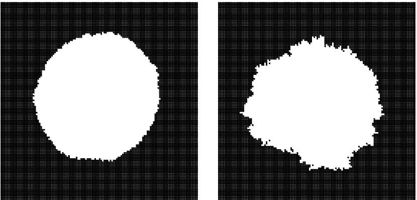
Figure 5.8: Snapshots of holes in an oxygen layer that have been formed by reaction with CO, In both cases the initial situation was a surface completely covered with oxygen except for one site, Diffusion of CO and reaction with oxygen are infinitely fast, but on the left the reaction is infinitely faster than the diffusion and on the right it is the other way around,

5.7 Lateral interactions

Lateral interactions are interactions between adsorbates, It is well-known that these interactions lead to structured adlayers at low temperatures, Recently, people have realized that the kinetics of surface reactions can be substantially affected by these interactions even at high temperature, Little is known about the form of these interactions and even less about the strength of them, In this section we present a general but not very efficient method, the method that is implemented in CARLOS to model pairwise additive interactions, and a few tricks to model more complicated interactions with reasonable efficiency, In all cases we assume that the lateral interactions are short range,

A general method to model lateral interaction consists of specifying the reaction and the occupation of the sites that may have adsorbates that will affect the reaction, For example, if we have a simple desorption of an adsorbate A on a square grid with a rate constant that depends on the occupation of the four neighboring sites, then we have the reactions

$$\matrix{&(0,1),\cr(-1,0),&(0,0),&(1,0),\cr&(0,-1)\cr} : \matrix{&*\cr*&\hbox{A}&*\cr&*\cr}\to\matrix{&*\cr*&*&*\cr&*\cr},$$

$$\matrix{&(0,1),\cr(-1,0),&(0,0),&(1,0),\cr&(0,-1)\cr} : \matrix{&*\cr*&\hbox{A}&\hbox{A}\cr&*\cr}\to\matrix{&*\cr*&*&\hbox{A}\cr&*\cr},$$

$$\matrix{&(0,1),\cr(-1,0),&(0,0),&(1,0),\cr&(0,-1)\cr} : \matrix{&\hbox{A}\cr*&\hbox{A}&\hbox{A}\cr&*\cr}\to\matrix{&\hbox{A}\cr*&*&\hbox{A}\cr&*\cr},$$ (5.46)

$$\matrix{&(0,1),\cr(-1,0),&(0,0),&(1,0),\cr&(0,-1)\cr} : \matrix{&*\cr\hbox{A}&\hbox{A}&\hbox{A}\cr&*\cr}\to\matrix{&*\cr\hbox{A}&*&\hbox{A}\cr&*\cr},$$

$$\matrix{&(0,1),\cr(-1,0),&(0,0),&(1,0),\cr&(0,-1)\cr} : \matrix{&\hbox{A}\cr\hbox{A}&\hbox{A}&\hbox{A}\cr&*\cr}\to\matrix{&\hbox{A}\cr\hbox{A}&*&\hbox{A}\cr&*\cr},$$

$$\matrix{&(0,1),\cr(-1,0),&(0,0),&(1,0),\cr&(0,-1)\cr} : \matrix{&\hbox{A}\cr\hbox{A}&\hbox{A}&\hbox{A}\cr&\hbox{A}\cr}\to\matrix{&\hbox{A}\cr\hbox{A}&*&\hbox{A}\cr&\hbox{A}\cr},$$

Of all symmetry-related reactions only one is shown, Each of these reactions can be given a different rate constant (or activation energy and preexponential factor), By specifying all possible occupations of the neighboring sites explicitly any form of the lateral interactions can be modeled, The disadvantage should also be clear, The list of reactions can be quite long, With $Z$ neighboring sites that may be occupied by an adsorbate that affects the reaction and $A$ possible occupations of each of these sites (including no adsorbate) there are $A^{Z}$ reactions to specify,

CARLOS (see section 4.3) has the possibility to deal with lateral interactions that change the activation energy of a reaction in a pairwise additive manner, Let’s take the previous example of a desorbing adsorbate A again, In CARLOS desorption can be specified as

$$\matrix{&(0,1),\cr(-1,0),&(0,0),&(1,0),\cr&(0,-1)\cr}:$$ (5.47)

$$\matrix{&\hbox{\{ $*$ A : $\varphi$ \}}\cr\hbox{\{ $*$ A : $\varphi$ \}}&\hbox{A}&\hbox{\{ $*$ A : $\varphi$ \}}\cr&\hbox{\{ $*$ A : $\varphi$ \}}\cr}\to\matrix{&\#\cr\#&*&\#\cr&\#\cr},$$

The notation with the curly braces means that an adsorbate A at the site changes the activation energy of the reaction by an amount $\varphi$, A vacant site does not change the activation energy, The hashes (#) on the right mean that the occupation of the site does not change, This way to model lateral interactions does not have the flexibility of the more general approach, but it is definitely much easier,

Figure 5.9 shows the typical effect of lateral interactions, Interactions between nearest neighbors are very often repulsive, On a square grid this leads the checkerboard structure at low temperatures, (Increasing the temperature leads to via an order-disorder phase transition to a random structure,) When diffusion is slow relaxation is slow and the checkerboard does not cover the whole system, but domains are formed, If one wants to get a good idea of these domains one can change the model in the following way, Instead of the reaction (5.47) one uses

$$\matrix{&(0,1),\cr(-1,0),&(0,0),&(1,0),\cr&(0,-1)\cr}:$$ (5.48)

$$\matrix{&\hbox{\{ $*2$ A2 : $\varphi$ \}}\cr\hbox{\{ $*2$ A2 : $\varphi$ \}}&\hbox{A1}&\hbox{\{ $*2$ A2 : $\varphi$ \}}\cr&\hbox{\{ $*2$ A2 : $\varphi$ \}}\cr}\to\matrix{&\#\cr\#&*1&\#\cr&\#\cr},$$

and

$$\matrix{&(0,1),\cr(-1,0),&(0,0),&(1,0),\cr&(0,-1)\cr}:$$ (5.49)

$$\matrix{&\hbox{\{ $*1$ A1 : $\varphi$ \}}\cr\hbox{\{ $*1$ A1 : $\varphi$ \}}&\hbox{A2}&\hbox{\{ $*1$ A1 : $\varphi$ \}}\cr&\hbox{\{ $*1$ A1 : $\varphi$ \}}\cr}\to\matrix{&\#\cr\#&*2&\#\cr&\#\cr},$$

In the initial condition if a site has a label ending in 1 (2) then a neighboring site should have a label ending in 2 (1), The reason for having two reactions representing effectively the same reaction is that one can now give neighboring sites on output a different coloring, If one gives “A1” to same color as “$*$2”, and “A2” the same color as “$*$1”, then all sites of one domain will have the same color as can be seen in Fig, 5.9, Completely covered or vacant areas will appear as a checkerboard now,

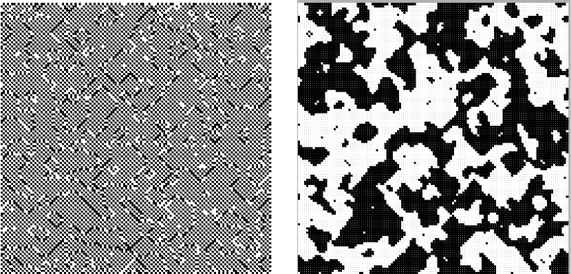
Figure 5.9: Snapshots of simulations of simple desorption with lateral interactions and no diffusion, Nearest neighbors repel each other, but next-nearest neighbors attract each other, On the left the adsorbates (in black) are shown for situation with half of the sites are occupied, On the right a similar situation is shown, but there the coloring of is reversed on alternate sites, So if a site is black when occupied and white when vacant, then a neighboring site is black when vacant and white when occupied,

For lateral interactions that are not pairwise additive we need not always use the general method, One should always look for some simple prescription describing the energetics, For example, suppose that the activation energy for simple desorption depends on the number of nearest-neighbor sites being occupied, Then this might be modeled by the reaction

$$(0,0/0),(0,0/1):\hbox{ A $n$}\to\hbox{$*$ $n$},$$ (5.50)

Here we have two sites per unit cell, The first is an actual site, but the second has a label that specifies how many of the neighbors of the actual site are occupied; i,e,, the label $n$ is number of adsorbates on neighboring sites, In CARLOS one can use infinitely fast reactions to update the labels specifying these numbers, but one can of course also implement this explicitly,

Another example would be simple desorption on a hexagonal grid with an activation energy that is affected by adsorbates that are nearest neighbors and that form equilateral triangles, For each real site we can defined two additional sites, If the translations of the unit cell are given by $a(1,0)$ and $a(1/2,1/2\sqrt{3})$, where $a$ is the unit cell parameter, then we can use site $(0,0/0)$ as real site, $(0,0/1)$ for the occupation of sites $(0,0/0)$, $(1,0/0)$, and $(0,1/0)$, and $(0,0/2)$ for the occupation of sites $(1,0/0)$, $(0,1/0)$, and $(1,1/0)$, The desorption can then be modeled in the notation of CARLOS as

$$(0,0/0),(0,0/1),(-1,0/2),(-1,0/1),(-1,-1/2),(0,-1/1),(0,-1/1):$$

A { no yes : $$\varphi \varphi \varphi$$} { no yes : } { no yes : }

{ no yes : $$\varphi \varphi \varphi$$} { no yes : } { no yes : }

$$\to\hbox{$*$ no no no no no no},$$ (5.51)

The label “yes” means that the three sites are all occupied, and the label “no” means that at least one is vacant, The activation energy depends linearly on the number of triangles formed by the adsorbates, and each triangle changes the adsorption energy by $\varphi$,

Chapter 6 Examples

This chapter is somewhat similar to chapter 5 on how to model reaction systems, However, the emphasize here is more on the information one can get from DMC simulations; i,e,, the reason why one wants to do DMC simulations instead of using conventional macroscopic rate equations,

6.1 The Ziff-Gulari-Barshad model

Although the work by Ziff, Gulari, and Barshad does not represent the first application of Monte Carlo to model surface reactions it is probably the most influential work of its type,[85] There are several reasons for that, It deals with CO oxidation which was and still is a very important process in catalysis and surface science, It is a very simple model, which makes it generic, Its simplicity also made it possible to analyze in detail the relation between the microscopic reactions and the macroscopic properties, It showed the shortcomings of the macroscopic rate equations and what the origin of these shortcomings were, It showed that these DMC simulations could yield so-called kinetic or non-equilibrium phase transitions, In fact, apart from the first-order phase transition also known from macroscopic rate equations, it showed that there was a continuous phase transition as well,

Figure 6.1: Phase diagram of the Ziff-Gulari-Barshad model, The coverages and the AB formation per unit time per site are shown as a function of the $y$ parameter,

We present here the model, which we will call the ZGB-model, in its generic form, There are two adsorbates; A and B, If one wants to use the ZGB-model for CO oxidation, then A stands for CO and B for atomic oxygen, There are three reactions in the model, Adsorbate A can adsorb at single vacant sites, Adsorbate B can adsorb, but as it forms diatomic molecules in the gas phase, two neighboring vacant sites are needed, An A will react with a B if they are nearest neighbors, This reactions is infinitely fast, so this takes place immediately after an adsorption, We can write the reaction as

$${\rm A(gas)}+* \to {\rm A(ads)}$$

$${\rm B}_{2}{\rm(gas)}+2* \to 2{\rm B(ads)}$$ (6.1)

$${\rm A(ads)}+{\rm B(ads)} \to {\rm AB(gas)}+2*$$

where $*$ is a vacant site, “ads” stands for an adsorbed species, and “gas” for a species in the gas phase, The reactions involving two sites can only take place on neighboring sites, Focusing on the sites only we have

$$* \to {\rm A}$$

$$2* \to 2{\rm B}$$ (6.2)

$${\rm A}+{\rm B} \to 2*$$

The adsorbates do not diffuse in the original model, and the grid is a square one, There are many extensions to this model dealing, amongst others, with desorption of CO and oxygen,[86] diffusion of the adsorbates,[86] an Eley-Rideal mechanism for the oxidation step, physisorption of the reactants, lateral interactions between the adsorbates,[86] blocking of the sites due to poisoning with lead or alloying,[87, 88] reconstruction of the surface (see section 6.5),[12, 13, 14, 82, 89, 90, 91, 92] and an inert adsorbate that causes oscillations,[93]

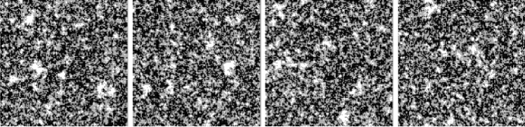
Figure 6.2: Snapshots of the adlayer in the Ziff-Gulari-Barshad model for $y=0.5255$ a value just below the first-order transition point, The black islands are formed by B’s, The A’s form the white islands,

The rate constant for adsorption of A can be derived as in section 3.2.3, and for adsorption of B as in section 3.2.7, The results are

$$W_{\rm A,ads} = {yPA_{\rm site}\sigma_{\rm A}\over\sqrt{2\pi mk_{\rm B}T}}$$ (6.3)

$$W_{\rm B,ads} = {2(1-y)PA_{\rm site}\sigma_{\rm B}\over 4\sqrt{2\pi mk_{\rm B}T}},$$ (6.4)

The $\sigma$’s are sticking coefficients, The quantity $y$ is the fraction of the molecules in the gas phase that are A’s, If we assume that the sticking coefficients are equal to each other, then we can simplify the rate constants to $y$ and $(1-y)/2$, respectively, by replacing time $t$ by $\tau=tPA_{\rm site}\sigma_{\rm A}/\sqrt{2\pi mk_{\rm B}T}$, We see that then the model depends only on one parameter; i,e,, only on $y$,

Simulations show that there are three states for the system, One possibility is that the surface is completely covered by A’s, There are no reactions that can take the system out of this state, Such a state is called on absorbing state in non-equilibrium statistical physics, In catalysis one talks in such a case of A poisoning, because it leads to the undesirable situation that the reactivity is zero, There is another absorbing state, but then with B poisoning, If the parameter $y$ is below a critical value $y_{1}$, then the system will always evolve into the B poisoning state, If the parameter $y$ is above another critical value $y_{2}$, then the system will always evolve into the A poisoning state, For $y<y_{1}$ there are so many ${\rm B}_{2}$ molecules in the gas phase that B adsorption will outcompete the A’s for the vacant sites that are formed by the reaction between the A’s and B’s, To same thing happens for $y>y_{2}$ except in this situations the A adsorption wins, At $y_{1}$ and at $y_{2}$ there is a kinetic or non-equilibrium phase transition,

For $y_{1}<y<y_{2}$ there is a third state with A’s and B’s on the surface and a non-zero reactivity, Figure 6.1 shows how the reactivity and the coverage depend on $y$, Note that all quantities change discontinuously at $y_{2}$, The phase transition at that value of $y$ is therefore called a first-order transition, At $y_{1}$ the quantities change continuously, so we have a continuous (or second-order) phase transition, Macroscopic rate equations also predict the first-order phase transition, but not the continuous one, However, the first-order phase transition is predicted by the macroscopic rate equations to be at $y_{1}=2/3$, whereas the best estimates from DMC simulations are $y_{2}=0.52560\pm 0.00001$,[94, 95] The continuous phase transition is estimated to be at $y_{1}=0.39065\pm 0.00010$,[96]

Figure 6.2 shows the reason for the discrepancy between the DMC results and those of macroscopic rate equations, The adlayer is definitely not a random mixture of adsorbates, The reason is that the fast reaction between the A’s and B’s, This reaction causes segregation of the adsorbates, Isolated A’s will not last long on the surface, because a B may adsorb on one of the vacant neighboring sites that will immediately react with the A which will remove the A from the surface, For a similar reason isolated B’s will be rare, Only islands of the same kind of adsorbate can last, because the particles in the center of an island have no neighboring sites onto which other particle can adsorb with which they will react, These islands are formed randomly, Islands of B are larger, They need be because A’s need only one vacant site for adsorption and can relatively easily break them up, Islands of A can be smaller, B’s need two neighboring vacant sites for adsorption and have more difficulty to remove A’s,

6.2 TPD/TPR of $2{\rm AB}\to{\rm A}_{2}+{\rm B}_{2}$

The model in this section illustrates how atomic details influence the kinetics, The AB molecule is adsorbed on the surface and the first reaction is the dissociation into an A and a B, This is only possible, however, if a neighboring site of the AB molecule is vacant, In the macroscopic rate equation

$${d\theta_{\rm AB}\over dt}=-k\theta_{\rm AB}\theta_{*},$$ (6.5)

we have dissociation as long as are molecule to dissociate and $\theta_{*}>0$, This means that if initially less than half the sites are occupied by AB’s all molecules can dissociate, In a DMC simulation things are not so straightforward, because the vacant sites might not be accessible, For example, the model here is applicable to NO reduction on rhodium, The nitrogen and oxygen atoms that are formed when NO dissociates do hardly diffuse at all, and severely restrict the motion of NO to find a vacant site,[97, 98]

Figure 6.3: Changes in the coverages (left) and rates of the reactions (right) for the $2{\rm AB}\to{\rm A}_{2}+{\rm B}_{2}$ process as a function of temperature (in Kelvin), The results are obtained from a simulation with a $256\times 256$ grid of a TPD/TPR experiment with a heating rate of $10\,{\rm K/sec}$ and an initial AB coverage of $0.4946\,$ML,

The model here has four reactions

$${\rm AB(ads)}+* \to {\rm A(ads)}+{\rm B(ads)},$$

$${\rm AB(ads)} \to {\rm AB(gas)}+*,$$ (6.6)

$$2{\rm A(ads)} \to {\rm A}_{2}{\rm(ads)}+2*,$$

$$2{\rm B(ads)} \to {\rm B}_{2}{\rm(ads)}+2*,$$

where $*$ is a vacant site, “ads” stands for an adsorbed species, and “gas” for a species in the gas phase, The reactions involving two sites can only take place on neighboring sites, Focusing only on the sites we have

$${\rm AB}+* \to {\rm A}+{\rm B},$$

$${\rm AB} \to *,$$ (6.7)

$$2{\rm A} \to 2*,$$

$$2{\rm B} \to 2*,$$

The kinetic parameters are $\nu_{\rm diss}=\nu_{\rm AB,des}=\nu_{\rm A,des}=\nu_{\rm B,des}=10^{13}\,\hbox{cm}^{-1}$, and $E_{\rm act,diss}/k_{\rm B}=11500\,$K, $E_{\rm act,AB,des}/k_{\rm B}=14500\,$K, $E_{\rm act,A,des}/k_{\rm B}=18000\,$K, and $E_{\rm act,B,des}/k_{\rm B}=21000\,$K, We see that the reactions above are ordered from fast to slow, In a TPD/TPR experiment they would also occur in that order if there would be no interference, We use a square grid for the simulations,

Figure 6.3 shows TPD/TPR spectra of the system and changes in the coverage, We see that AB dissociation starts at low temperature, but not all of the AB dissociates even though there are enough vacant sites, This means that the available sites are not accessible; the A’s and B’s prevent the AB molecules from reaching the vacant sites, At about $T=450\,$K the AB molecules that are still present start to desorb, This leads to new vacant sites which can be used for dissociation, At this temperature the dissociation is almost instantaneous, From the changes in the coverages and the reaction rates we can see that also not all new vacant sites are used for dissociation, The mobility of the A’s and B’s is still too low for AB’s to reach all vacant sites, At $T=550\,$K all AB’s are gone and we have associative desorption of ${\rm A}_{2}$ and at higher temperature of ${\rm B}_{2}$,

6.3 TPD with strong repulsive interactions

One of the clearest examples of the advantage of DMC simulations over macroscopic rate equations is formed by simple desorption with strong lateral interactions, If we take for example a square grid, an initial situation with all sites occupied, and repulsive interactions between nearest neighbors, then the following happens, Initially, each adsorbate has the same tendency to desorb, However, if one adsorbate desorbs then its former neighbors suddenly feel less repulsion and become adsorbed more strongly, This means that desorption takes place in two stages, First about half the adsorbates desorb, because they have many neighbors, After these adsorbates have desorbed the structure of the adlayer is that of a checkerboard, with almost all adsorbates having no neighbors, Because these adsorbates feel little or no repulsion from other adsorbates they desorb at a later stages,

Figure 6.4: Temperature-Programmed Desorption spectrum (desorption rate vs, temperature in Kelvin) of adsorbates repelling each other, The fat line is the total desorption rate, The thin lines are separate contributions of adsorbates desorbing with a number of nearest neighbors given by the number next to the curve, Activation energy for desorption is $E_{\rm act}/k_{\rm B}=14590\,$K and the preexponential factor is $\nu=1.435\cdot 10^{12}\,\hbox{cm}^{-1}$, These numbers were taken from CO desorption from Rh(100) at low coverage, The repulsion between two adsorbates is $1000\,$K,

Note that the process involves a symmetry breaking, Initially all sites are equivalent, but after half the adsorbates have desorbed alternate sites are occupied and vacant, Ordinary macroscopic rate equations are not able to describe this symmetry breaking, because they assume that all site are equivalent during the whole process, We can split the macroscopic rate equations in two; one for the sites with the adsorbates that desorb first, and one for the sites with adsorbates that desorb later, However, the equations for both sites are equivalent and the symmetry breaking only occurs if the initial situation already has a small difference in the occupations between the sites with the early desorbers and the sites with the late desorbers, For DMC simulations such an unrealistic initial condition is not necessary, In DMC fluctuations in the times when reactions occur cause the symmetry breaking as they do in real systems, Such fluctuations are not included in macroscopic rate equations,

The fluctuations determine which adsorbates desorb first, and also affect the structure of the adlayer when the coverage has been more of less halved, A perfect checkerboard structure is only found when the adsorbates also diffuse fast and when the temperature is well below the order-disorder phase transition temperature, For small system sizes the diffusion need not be so fast as for large system sizes, Diffusion has to make sure that no domains are formed as in figure 5.9, Simulations show that even at relatively small systems with say a $128\times 128$ grid it is almost impossible to avoid domain formation,

Figure 6.4 shows a TPD spectrum for a system with repulsive interactions, We show TPD instead of isothermal desorption, because the latter shows the two stages in the desorption only in how fast the coverage and the desorption rate decreases, If the coverage is plotted logarithmically, then we get first a straight line with a large negative slope, followed by a straight line with a small, in absolute sense, negative slope, In TPD the two stages are much clearer, because the desorption rate has two peaks, The figure shows that the second stage (i,e,, the second peak) has also contributions from adsorbates with one, two, and even three neighbors, which is due to the fact that the first stage never forms a perfect checkerboard structure, If the repulsion becomes very strong, then more than two peaks can be formed,

In real systems the effects of lateral interactions are generally not so unambiguous, The lateral interactions have to be strong enough so that a well-defined structure is formed when half the adsorbates have desorbed, If this is not the case then the lateral interactions only show up by shifting or broadening a single peak when the initial coverage is increased, When lateral interactions are strong enough, then they may also push adsorbates to other adsorption sites, These sites have a lower adsorption energy, but overall the energy is lowered because it lessens the repulsion between the adsorbates, The result may even be an adlayer structure that is incommensurate with the substrate, Finally, lateral interactions need not just be between nearest neighbors, Interactions between next- en next-next-nearest neighbors are not uncommon, Longer range interactions have been excluded,[99] but charged adsorbates might have long-range interactions, which may explain very broad desorption peaks,

6.4 CO electrooxidation on a Pt-Ru electrode

The reason for doing DMC simulations is that the system is not homogeneous, This may be because the reactions cause an inhomogeneity in the adlayer, but it may also be that the substrate is inhomogeneous as in the case for the system of this section, The precise structure of the Pt-Ru electrode is not known, We will assume here that the two metals each form large islands mainly for illustrative purposes,[100] The idea of having two metals is that each catalyzes only some reactions well, In the model here the ${\rm CO}_{2}$ formation proceeds well on Pt and the ${\rm H}_{2}{\rm O}$ dissociates on Ru,

Figure 6.5: Current of CO electrooxidation as a function of electrode potential for pure Pt, pure Ru, and a Pt-Ru alloy with randomly distributed Pt and Ru atoms, The initial surface is for about 99% covered by CO and the potential is $-0.2\,$V, The potential is increased by $0.1\,$V/sec,

We model the system with a square grid, We simulate a linear-sweep voltammetry experiment in which the electrode is initially for 99% covered by CO, The following reactions can occur,

$${\rm H}_{2}{\rm O}+* \to {\rm OH}+{\rm H}^{+}+e^{-},$$

$${\rm OH}+{\rm H}^{+}+e^{-} \to {\rm H}_{2}{\rm O}+*,$$ (6.8)

$${\rm CO}+{\rm OH} \to {\rm CO}_{2}+2*+{\rm H}^{+}+e^{-},$$

or if we just look at the site occupation

$$* \to {\rm OH},$$

$${\rm OH} \to *,$$ (6.9)

$${\rm CO}+{\rm OH} \to 2*,$$

The reactions can take place on both metals, and the latter also on the border of a Pt and a Ru patch, The CO diffuses rapidly over the surface, whereas OH remains fixed at the site where it is formed, In the experiment the current is measured; i,e,, the sum of the rates of the first and the last reaction minus the second,

Although the reactions can occur on both metals, the rate constants differ, We can write the rate constants as

$$W_{\rm ads}^{\rm M} = k_{\rm ads}^{\rm M}\exp\left[{\alpha_{\rm M}e_{0}E\over k_{\rm B}T}\right],$$

$$W_{\rm des}^{\rm M} = k_{\rm des}^{\rm M}\exp\left[-{(1-\alpha_{\rm M})e_{0}E\over k_{\rm B}T}\right],$$ (6.10)

$$W_{\rm rx}^{{\rm M}_{1}{\rm M}_{2}} = k_{\rm rx}^{{\rm M}_{1}{\rm M}_{2}}\exp\left[{\alpha_{{\rm M}_{1}{\rm M}_{2}}e_{0}E\over k_{\rm B}T}\right],$$

The first refers to the dissociative adsorption of water, the second to the desorption of water, and the last to the formation of ${\rm CO}_{2}$, In the last ${\rm M}_{1}$ is the metal with the CO, and ${\rm M}_{2}$ the metal with the OH, The $\alpha$’s are so-called transfer coefficients, $e_{0}$ is the elementary charge, and $E$ is the potential of the electrode, All transfer coefficient are taken equal to 0.5, $T=300\,$K, and $k_{\rm ads}^{\rm Pt}=0.2\,{\rm s}^{-1}$, $k_{\rm des}^{\rm Pt}=10^{4}\,{\rm s}^{-1}$, $k_{\rm ads}^{\rm Ru}=40\,{\rm s}^{-1}$, $k_{\rm des}^{\rm Ru}=5\,{\rm s}^{-1}$, $k_{\rm rx}^{\rm RuRu}=0.1\,{\rm s}^{-1}$, $k_{\rm rx}^{\rm RuPt}=0.1\,{\rm s}^{-1}$, $k_{\rm rx}^{\rm PtPt}=1\,{\rm s}^{-1}$, and $k_{\rm rx}^{\rm PtRu}=1\,{\rm s}^{-1}$, The rate constant for CO diffusion is $100\,{\rm s}^{-1}$,

Figure 6.5 shows the voltammograms for a Pt, a Ru, and a Pt-Ru electrode, These are obtained by linearly changing the potential of the electrode from $-0.2\,$ to $0.5\,$V in $7\,$seconds, The remarkable fact is that the Pt-Ru alloy is more reactive than either of the pure metals, The reason for this is as follows, The rate limiting step on Pt is the dissociative adsorption of water, On Ru the rate limiting step is the formation of ${\rm CO}_{2}$, We get a synergetic effect if the oxidation step on the boundary of the Pt and Ru parts of the alloy is at least as fast as on Pt, In that case OH is formed on Ru on the boundary, and CO on Pt reacts with this OH, This is most clearly seen when we do a simulation with large Pt and Ru islands (see figure 6.6), There is a depletion of CO on Pt near the boundary, because there the CO react, There is a higher concentration of OH on Ru near the boundary because the higher oxidation reactivity there leads to more vacant sites for water adsorption,

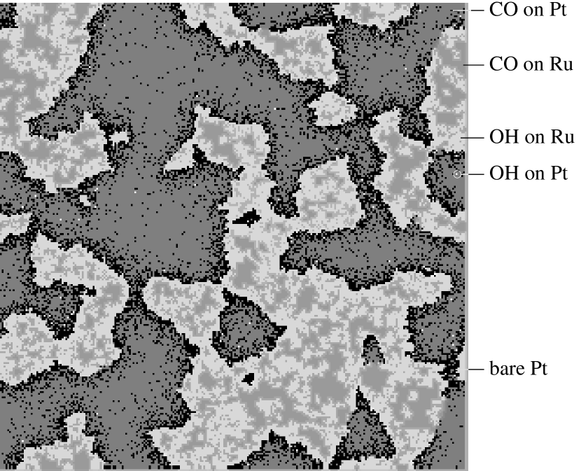
Figure 6.6: Snapshot of CO electrooxidation on a Pt-Ru electrode that consists of large islands of Pt and large islands of Ru,

6.5 Oscillations of CO oxidation on Pt surfaces

One problem for which extensive DMC simulations have been done by various groups is the problem of CO oscillations on Pt(100) and Pt(110), A crucial role in these oscillations is played by the reconstruction of the surface, and the effect of this reconstruction on the adsorption of oxygen, The explanation of the oscillations is as follows, A bare Pt surface reconstructs into a structure with a low sticking coefficient for oxygen, This means that predominantly CO adsorbs on bare Pt, However, CO lifts the reconstruction, The normal structure has a high sticking coefficient for oxygen, So after CO has adsorbed in a sufficient amount to lift the reconstruction oxygen can also adsorb, The CO and the oxygen react, and form ${\rm CO}_{2}$, This ${\rm CO}_{2}$ rapidly desorbs leaving bare Pt which reconstructs again, An important aspect of this process, and also other oscillatory reactions on surfaces, is the problem of synchronization, The cycle described above can easily take place on the whole surface, but oscillations on different parts on the surface are not necessarily in phase, and the overall reactivity of a surface is then constant, To get the whole surface oscillating in phase there has to be a synchronization mechanism,

The most successful model to describe oscillations on Pt surfaces is the one by Kortlüke, Kuzovkov, and von Niessen,[13, 14, 82, 90, 91, 92] This model has CO adsorption and desorption, oxygen adsorption, ${\rm CO}_{2}$ formation, CO diffusion, and surface reconstruction, The surface is modeled by a square grid, Each site in the model is either in state $\alpha$ or in state $\beta$, The $\alpha$ state is the reconstructed state which has a reduced sticking coefficient for oxygen, The $\beta$ state is the unreconstructed state with a high sticking coefficient for oxygen, An $\alpha$ site will convert a neighboring $\beta$ site into an $\alpha$ state if neither sites is occupied by CO, A $\beta$ site will convert a neighboring $\alpha$ site into $\beta$ if at least one of them is occupied by CO,

The model shows a large number of phenomena depending on the rate constants, We will only look at oscillations that occur for reduced rate constants $y=0.494$, $k=0.1$, and $V=1$,[101] The first rate constant, $y$, is the one for CO adsorption and has the same meaning as in the ZGB-model (see section 6.1), The second, $k$, is the rate constant for CO desorption, The last, $V$, is the rate constant for the reconstruction and the lifting of the reconstruction, The rate constant for oxygen adsorption is as for the ZGB-model $(1-y)/2$ on the $\beta$ phase, and $s_{\alpha}(1-y)/2$ on the $\alpha$ phase, We will look at the Pt(110) surface which has $s_{\alpha}=\,0.5$, The diffusion rate constant has been varied,

Figure 6.7 shows snapshots obtained from some large simulations in which the diffusion is just about fast enough to lead to global oscillations provided the initial conditions are favorable, However, it is also possible to choose the initial conditions so that the oscillations are not synchronized properly, In that case one can see the formation of patterns as the right half of the figure shows,

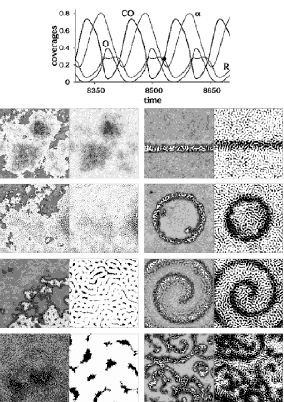
Figure 6.7: Global oscillations and pattern formation with $D=250$, The top shows temporal variations of the coverages, the fraction of the substrate in the $\alpha$ phase, and the ${\rm CO}_{2}$ production $R$, Each picture has two parts, In the left part we plot the chemical species; CO particles are grey and O particles are white, and empty sites are black, The right part shows the structure of the surface; $\alpha$ phase sites are black, and $\beta$ phase sites are white, Sections of the upper-left corner with $L=8192$, $4096$, $1024$, and $256$ are shown on the left half of the figure, The sections correspond to the dot in the temporal plot at the top, On the right half of the figure we have a wave front, a target, a spiral, and turbulence ($L=2048$), which can be obtained with different initial conditions,

Synchronization is obtained when the diffusion rate is fast enough, The minimal value is related to the so-called Turing-like structures that are formed in the substrate, These structure can best be seen in the lower two pictures on the left and all pictures on the right of figure 6.7, If diffusion is so fast that within one oscillatory period CO can move from one phase ($\alpha$ or $\beta$) to a neighboring island of the other phase, then the oscillation are well synchronized, If the diffusion rate is slower, then we get pattern formation, Note that the system has two length scales, The characteristic length scale of the adlayer is much larger than the characteristic length scale of the Turing-like structures as can be seen in the right half of the figure,

Bibliography

- [1] M. P. Allen and D. J. Tildesley, Computer Simulation of Liquids (Clarendon, Oxford, 1987).
- [2] A. Zangwill, Physics at Surfaces (Cambridge University Press, Cambridge, 1988).
- [3] J. M. Thomas and W. J. Thomas, Principles and Practice of Heterogeneous Catalysis (VCH, Weinheim, 1997).
- [4] N. W. Ashcroft and N. D. Mermin, Solid State Physics (Holt, Rinehart, and Winston, New York, 1976).
- [5] N. V. Petrova and I. N. Yakovkin, Lateral Interaction and CO Adlayer Structures on the Pt(111) Surface, Surf. Sci. 519 (2002) 90.
- [6] C.-T. Kao, G. S. Blackman, M. A. V. Hove, G. A. Somorjai, and C.-M. Chan, The Surface Structure and Chemical Reactivity of Rh(111)-(22)-3NO by HREELS and Dynamical LEED Analysis, Surf. Sci. 224 (1989) 77.
- [7] M. van Hardeveld, Elementary Reactions in the Catalytic Reduction of NO on Rhodium Surfaces, Ph.D. thesis, Eindhoven University of Technology (1997).
- [8] S. Dahl, A. Logadottir, R. C. Egeberg, J. H. Larsen, I. Chorkendorff, E. Törnqvist, and J. K. N. rskov. Role of Steps in Activation on Ru(0001), Phys. Rev. Lett. 83 (1999) 1814.
- [9] B. Hammer, Bond Activation at Monatomic Steps: NO Dissociation at Corrugated Ru(0001), Phys. Rev. Lett. 83 (2000) 3681.
- [10] R. Imbihl and G. Ertl, Oscillatory Kinetics in Heterogeneous Catalysis, Chem. Rev. 95 (1995) 697.
- [11] M. M. Slin’ko and N. I. Jaeger, Oscillating Heterogeneous Catalytic Systems, Studies in Surface Science and Catalysis 86 (Elsevier, Amsterdam, 1994).
- [12] R. J. Gelten, A. P. J. Jansen, R. A. van Santen, J. J. Lukkien, J. P. L, Segers, and P. A. J. Hilbers. Monte Carlo Simulations of a Surface Reaction Model Showing Spatio-Temporal Pattern Formation and Oscillations, J. Chem. Phys. 108 (1998) 5921.
- [13] V. N. Kuzovkov, O. Kortlücke, and W. von Niessen, Nucleation and Island Growth Kinetics on Reconstructing Surfaces, Phys. Rev. Lett. 83 (1999) 1636.
- [14] O. Kortlücke, V. N. Kuzovkov, and W. von Niessen, Global Synchronization via Homogeneous Nucleation in Oscillating Surface Reactions, Phys. Rev. Lett. 83 (1999) 3089.
- [15] M. Gruyters, T. Ali, and D. A. King, Modelling temporal kinetic oscillations for CO oxidation on Pt{100}. The -CO island growth rate power law model, Chem. Phys. Lett. 232 (1995) 1.
- [16] M. Gruyters, T. Ali, and D. A. King, Theoretical inquiry into the microscopic origins of the oscillatory CO oxidation reaction on Pt{100}, J. Phys. Chem. 100 (1996) 14417.
- [17] A. R. Leach, Molecular Modelling. Principles and Applications (Longman, Singapore, 1996).
- [18] J. C. Keck, Variational Theory of Chemical Reaction Rates Applied to Three-Body Recombinations, J. Chem. Phys. 32 (1960) 1035.
- [19] J. C. Keck, Statistical Investigation of Dissociation Cross-Section for Diatoms, Discuss. Faraday Soc. 33 (1962) 173.
- [20] J. C. Keck, Variational Theory of Reaction Rates, Adv. Chem. Phys. 13 (1967) 85.
- [21] P. Pechukas, Statistical Approximations in Collision Theory, In W. Miller (ed.), Dynamics of Molecular Collisions, Part B, 269–322 (Plenum Press, New York, 1976).
- [22] D. G. Truhlar, A. D. Isaacson, and B. C. Garrett, Generalized Transition State Theory, In M. Baer (ed.), Theory of Chemical Reaction Dynamics, Part IV, 65–138 (CRC Press, Boca Raton, 1985).
- [23] W. H. Miller, Quantum Mechanical Transition State Theory and a New Semiclassical Model for Reaction Rate Constants, J. Chem. Phys. 61 (1974) 1823.
- [24] W. H. Miller, Semiclassical Limit of Quantum Mechanical Transition State Theory for Nonseparable Systems, J. Chem. Phys. 62 (1975) 1899.
- [25] G. A. Voth, Feynman Path Integral Formulation of Quantum Mechanical Transition-State Theory, J. Phys. Chem. 97 (1993) 8365.
- [26] V. A. Benderskii, D. E. Makarov, and C. A. Wight, Chemical Dynamics at Low Temperatures, Adv. Chem. Phys. 88 (1994) 1.
- [27] D. A. McQuarrie, Statistical Mechanics (Harper, New York, 1976).
- [28] R. Becker, Theorie der Wärme (Springer, Berlin, 1985).
- [29] A. P. J. Jansen, Compensating Hamiltonian Method for Chemical Reaction Dynamics: Xe Desorption from Pd(100), J. Chem. Phys. 94 (1991) 8444.
- [30] E. Kreyszig, Advanced Engineering Mathematics (Wiley, New York, 1993).
- [31] A. H. Zemanian, Distribution Theory and Transform Analysis (Dover, New York, 1987).
- [32] R. A. van Santen and J. W. Niemantsverdriet, Chemical Kinetics and Catalysis (Plenum Press, New York, 1995).
- [33] P. G. Mezey, Potential Energy Hypersurfaces (Elsevier, Amsterdam, 1987).
- [34] E. K. Grimmelmann, J. C. Tully, and E. Helfand, Molecular Dynamics of Infrequent Events: Thermal Desorption of Xenon from a Platinum Surface, J. Chem. Phys. 74 (1981) 5300.
- [35] J. C. Tully, Dynamics of gas-surface interactions: Thermal desorption of Ar and Xe from platinum, Surf. Sci. 111 (1981) 461.
- [36] E. B.Wilson, J. C. Decius, and P. C. Cross, Molecular Vibrations: The Theory of Infrared and Raman Vibrational Spectra (McGraw-Hill, London, 1955).
- [37] H. Goldstein, Classical Mechanics (Addison-Wesley, Amsterdam, 1981).
- [38] A. Messiah, Quantum Mechanics (North-Holland, Amsterdam, 1961).
- [39] P. Hohenberg and W. Kohn, Inhomogeneous Electron Gas, Phys. Rev. 136 (1964) B864.
- [40] W. Kohn and L. S. Sham, Self-Consistent Equations Including Exchange and Correlation Effects, Phys. Rev. 140 (1965) A1133.
- [41] R. G. Parr and W. Yang, Density-Functional Theory of Atoms and Molecules (Oxford University Press, New York, 1989).
- [42] M. Abramowitz and I. A. Stegun, Handbook of Mathematical Functions with Formulas, Graphs, and Mathematical Tables (Dover, New York, 1965).
- [43] A. P. J. Jansen, Monte Carlo Simulations of Chemical Reactions on a Surface with Time-Dependent Reaction-Rate Constants, Comput. Phys. Comm. 86 (1995) 1.
- [44] A. M. de Jong and J. W. Niemantsverdriet, Thermal desorption analysis: Comparative test of ten commonly applied procedures, Surf. Sci. 233 (1990) 355.
- [45] G. A. Somorjai, Introduction to surface chemistry and catalysis (Wiley, Chichester, 1993).
- [46] A. Cassuto and D. A. King, Rate Expressions for Adsorption and Desorption Kinetics with Precursor States and Lateral Interactions, Surf. Sci. 102 (1981) 388.
- [47] K. Binder, Monte Carlo Methods in Statistical Physics (Springer, Berlin, 1986).
- [48] D. T. Gillespie, A general method for numerically simulating the stochastic time evolution of coupled chemical reactions, J. Comput. Phys. 22 (1976) 403.
- [49] D. T. Gillespie, Exact stochastic simulations of coupled chemical reactions, J. Phys. Chem. 81 (1977) 2340.
- [50] J. Honerkamp, Stochastische Dynamische Systeme (VCH, Weinheim, 1990).
- [51] A. P. J. Jansen and J. J. Lukkien, Dynamic Monte-Carlo Simulations of Reactions in Heterogeneous Catalysis, Catalysis Today 53 (1999) 259.
- [52] D. T. Gillespie, Approximate Accelerated Stochastic Simulation of Chemically Reacting Systems, J. Chem. Phys. 115 (2001) 1716.
- [53] H. Resat, H. S. Wiley, and D. A. Dixon, Probability Weighted Dynamic Monte Carlo Method for Reaction Kinetics Simulations. Submitted to J. Chem. Phys. B (2001).
- [54] K. A. Fichthorn and W. H. Weinberg, Theoretical Foundations of Dynamical Monte Carlo Simulations, J. Chem. Phys. 95 (1991) 1090.
- [55] H. C. Kang and W. H. Weinberg, Kinetic modeling of surface rate processes, Surf. Sci. 299/300 (1994) 755.
- [56] B. Meng and W. H. Weinberg, Monte Carlo Simulations of Temperature-Programmed Desorption Spectra, J. Chem. Phys. 100 (1994) 5280.
- [57] F. C. Alcaraz, M. Droz, M. Henkel, and V. Rittenberg, Reaction-Diffusion Processes, Critical Dynamics, and Quantum Chains, J. Phys. 230 (1994) 250.
- [58] W. Feller, An Introduction to Probability Theory and Its Applications (Wiley, New York, 1970).
- [59] D. E. Knuth, The Art of Computer Programming, Volume III: Sorting and Searching (Addison-Wesley, Reading, 1973).
- [60] I. Mitrani, Simulation Techniques for Discrete Event Systems (Cambridge University Press, Cambridge, 1982).
- [61] J. J. Lukkien, J. P. L. Segers, P. A. J. Hilbers, R. J. Gelten, and A. P. J, Jansen. Efficient Monte Carlo Methods for the Simulation of Catalytic Surface Reactions, Phys. Rev. E 58 (1998) 2598.
- [62] J. P. L. Segers, Algorithms for the Simulation of Surface Processes. Ph.D. thesis, Eindhoven University of Technology (1999).
- [63] D. E. Knuth, The Art of Computer Programming, Volume I: Fundamental Algorithms (Addison-Wesley, Reading, 1973).
- [64] A. P. J. Jansen, A Monte Carlo Study of Temperature-Programmed Desorption With Lateral Attractive Interactions, Phys. Rev. B 52 (1995) 5400.
- [65] R. M. Nieminen and A. P. J. Jansen, Monte Carlo Simulations of Surface Reactions, Appl. Catal. A: General 160 (1997) 99.
- [66] M. T. M. Koper, J. J. Lukkien, A. P. J. Jansen, P. A. J. Hilbers, and R. A. va, Santen. Monte Carlo Simulations of a Simple Model for the Electrocatalytic CO Oxidation on Platinum, J. Chem. Phys. 109 (1998) 6051.
- [67] S. J. Lombardo and A. T. Bell, A Review of Theoretical Models of Adsorption, Diffusion, Desorption, and Reaction of Gases on Metal Surfaces, Surf. Sci. Rep. 13 (1991) 1.
- [68] V. Privman, Nonequilibrium Statistical Mechanics in One Dimension (Cambridge University Press, Cambridge, 1997).
- [69] J. Mai and W. von Niessen, Cellular-automaton approach to a surface reaction, Phys. Rev. A 44 (1991) R6165.
- [70] J. Mai and W. von Niessen, Diffusion and reaction in multicomponent systems via cellular-automaton modeling: , J. Chem. Phys. 98 (1993) 2032.
- [71] R. Danielak, A. Perera, M. Moreau, M. Frankowicz, and R. Kapral, Surface Structure and Catalytic CO Oxidation Oscillations, Physica A 229 (1996) 428.
- [72] J. P. Boon, B. Dab, R. Kapral, and A. Lawniczak, Lattice Gas Automata for Reactive Systems, Phys. Rep. 273 (1996) 55.
- [73] J. R. Weimar, Simuation with Cellular Automata (Logos Verlag, Berlin, 1997).
- [74] S. Wolfram, A New Kind of Science (Wolfram Media, Champaign, Illinois, 2002).
- [75] B. Drossel, Self-Organized Criticality and Synchronization in the Forest-Fire Model, Los Alamos Preprint Server; http://xxx.lanl.gov, paperno. cond-mat/9506021 (1995).
- [76] CARLOS is a general-purpose program, written in C by J. J. Lukkien, fo, simulating reactions on surfaces that can be represented by regular grids; an implementation of the First-Reaction Method, the Variable Stepsize Method, and the Random Selection Method, http://wwwpa.win.tue.nl/johanl/carlos/.
- [77] W. H. Press, B. P. Flannery, S. A. Teukolsky, and W. T. Vetterling, Numerical Recipes. The Art of Scientific Computing (Cambridge University Press, Cambridge, 1989).
- [78] J. Stoer and R. Bulirsch, Introduction to Numerical Analysis (Springer, New York, 1993).
- [79] S. Redner, Scaling Theories of Diffusion-Controlled and Ballistically Controlled Bimolecular Reactions, In V. Privman (ed.), Nonequilibrium Statistical Mechanics in One Dimension, 3–27 (Cambridge University Press, Cambridge, 1996).
- [80] A. A. Ovchinnikov and Y. B. Zeldovich, Role of Density Fluctuations in Bimolecular Reaction Kinetics, Chem. Phys. 28 (1978) 215.
- [81] D. Toussaint and F. Wilczek, Particle-Antiparticle Annihilation in Diffusive Motion, J. Chem. Phys. 78 (1983) 2642.
- [82] V. N. Kuzovkov, O. Kortlücke, and W. von Niessen, Kinetic Model for Surface Reconstruction, Phys. Rev. E 66 (2002) 011603.
- [83] V. P. Zhdanov and B. Kasemo, ??, J. Catal. 170 (1997) 377.
- [84] V. P. Zhdanov and B. Kasemo, Kinetics of the Reaction Complicated by Spatial Constraints for Adsorption, Formation of Islands, and Steps, Surf. Sci. 412/413 (1998) 527.
- [85] R. M. Ziff, E. Gulari, and Y. Barshad, Kinetic Phase Transitions in an Irreversible Surface-Reaction Model, Phys. Rev. Lett. 56 (1986) 2553.
- [86] H.-P. Kaukonen and R. M. Nieminen, Computer simulation studies of the catalytic oxidation of carbon monoxide on platinum metals, J. Chem. Phys. 91 (1989) 4380.
- [87] J.-P. Hovi, J. Vaari, H.-P. Kaukonen, and R. M. Nieminen, Simulations of the effect of preadsorbed poisons and promoters on irreversible surface reactions, Comput. Mater. Sci. 1 (1992) 33.
- [88] J. Mai, A. Casties, W. von Niessen, and V. N. Kuzovkov, A Stochastic Model and a Monte Carlo Simulation for the Description of CO Oxidation on Pt/Sn Alloys, J. Chem. Phys. 102 (1995) 5037.
- [89] R. J. Gelten, R. A. van Santen, and A. P. J. Jansen, Dynamic Monte Carlo Simulations of Oscillatory Heterogeneous Catalytic Reactions, In P. B. Balbuena and J. M. Seminario (eds.), Molecular Dynamics: From Classical to Quantum Methods (Elsevier, Amsterdam, 1999).
- [90] O. Kortlücke, V. N. Kuzovkov, and W. von Niessen, Oscillation Phenomena Leading to Chaos in a Stochastic Surface Reaction Model, Phys. Rev. Lett. 81 (1998) 2164.
- [91] V. N. Kuzovkov, O. Kortlücke, and W. von Niessen, Kinetic Oscillations in the Catalytic CO Oxidation on Pt Single Crystal Surfaces: Theory and Simulations, J. Chem. Phys. 108 (1998) 5571.
- [92] O. Kortlücke, V. N. Kuzovkov, and W. von Niessen, Simulation of Kinetic Oscillations in Surface Reactions on Reconstructing Surfaces, J. Chem. Phys. 110 (1999) 11523.
- [93] N. M. H. Janssen, P. D. Cobden, and B. E. Nieuwenhuys, Non-linear behaviour of nitric oxide reduction reactions over metal surfaces, J. Phys. Condens. Matter 9 (1997) 1889.
- [94] R. M. Ziff and B. J. Brosilow, Investigation of the first-order phase transition in the reaction model using a constant-coverage kinetic ensemble, Phys. Rev. A 46 (1992) 4630.
- [95] B. J. Brosilow, E. Gulari, and R. M. Ziff, Boundary effects in a surface reaction model for CO oxidation, J. Chem. Phys. 98 (1993) 674.
- [96] I. Jensen, H. Fogedby, and R. Dickman, Critical Exponents for an Irreversible Surface Reaction Model, Phys. Rev. A 41 (1990) 3411.
- [97] R. M. van Hardeveld, M. J. P. Hopstaken, J. J. Lukkien, P. A. J. Hilbers, A. P. J. Jansen, R. A. van Santen, and J. W. Niemantsverdriet. Role of Surface Diffusion in the Ordering of Adsorbed Molecules: Dynamic Monte Carlo Simulations of NO on Rh(111), Chem. Phys. Lett. 302 (1999) 98.
- [98] A. P. J. Jansen, C. G. M. Hermse, F. Fréchard, and J. J. Lukkien, Ab-initio kinetics of heterogeneous catalysis: NO+N+O/Rh(111). In V. Alexandrov, J. Dongarra, B. Juliano, R. Renner, and C. Ta, (eds.), Computational Science—ICCS 2001, 531–540 (Springer, Berlin, 2001).
- [99] Q. Ge, R. Kose, and D. A. King, Adsorption Energetics and Bonding from Femtomole Calorimetry and from First Principles Theory, Adv. Catal. 45 (2000) 207.
- [100] M. T. M. Koper, J. J. Lukkien, A. P. J. Jansen, and R. A. van Santen, Lattice Gas Model for CO Electrooxidation on Pt-Ru Bimetallic Surfaces, J. Phys. Chem. B 103 (1999) 5522.
- [101] R. Salazar, A. P. J. Jansen, and V. N. Kuzovkov, A New Synchronization Mechanism Via Turing-Like Microscopic Structures for CO Oxidation on Pt(110), Los Alamos Preprint Server; http://arXiv.org/, paperno. cond-mat/0210699 (2002).